Comparing Risk Neutral Density Estimation
Methods using Simulated Option Data
Amine Bouden
∗Abstract—In this paper I use Monte Carlo simu-lated option data to investigate the empirical power of six Risk Neutral Density (RND) estimation tech-niques. Three alternative approaches are used for comparison and the choice of the most suitable method depends on: their performance to correctly price options, their capacity to fit the true density which is estimated from the underlying asset series -and their ability to forecast the future realization of the underlying asset. I found that the decision de-pends on the purpose of the framework: for pricing purpose, the interpolation techniques would be ade-quate. However, if the aim is to extract market ex-pectations, the Edgeworth expansion should be used.
Keywords: Risk Neutral Density, Monte Carlo simu-lation, Probability Integral Transform
1
Introduction
Options traded on financial assets allow market partic-ipants to take views on the future values of the assets themselves. This projection towards the future confers to the option a sort of forward-looking information on the future evolution of the underlying assets. For example, in the case of Call option, the larger today’s premium is, the higher is the probability to exert the option and greater is the likelihood that the asset price finishes above the strike price at maturity. These probabilities, taken together, form the so-called implied Probability Density Function also referred as Risk Neutral Density function (henceforth RND). More precisely, when the market operators eval-uate theoretically an option price, they formulate their own estimates of these probabilities and their ’feelings’ about future evolutions of the underlying asset are sum-marized in the RND. The reason why it is called ’Risk Neutral’ density is that because it is estimated in a risk neutral world (in opposition with the real world) under which all investors are assumed to have no risk prefer-ences. A relatively large number of estimation methods has been proposed in the empirical literature and almost all are based on one of the following approaches:
i. Assuming that the underlying asset follows a partic-ular stochastic process and constructing the RND
∗University of Paris 2 Pantheon-Assas - ERMES - CNRS, 12
Place Panthon 75 230 Paris Cedex 5, Tel: +33 6 81 76 16 49, Email: [email protected]
from the estimated process (Geometric Brownian Motion giving the lognormal distrbution as a RND).
ii. Fitting a particular parametric form for the density which would reflect as well as possible the market conditions (mixture of 2 lognormals or the Edge-worth expansion).
iii. Using interpolation techniques to smooth the Call pricing function. The RND is then obtained by nu-merical differentiation (2 interpolation methods in spaces (volatility / strike) and (volatility / delta)).
iv. Semi-parametric techniques based on implied bino-mial trees.
Given these alternative techniques, a question arises: ’what about their reliability?’ Numerous comparison tools dealing with the stability and the accuracy of the estimated RND were considered: [1] tested the relative stability of the alternative RNDs and their robustness to small perturbations. [3] chose to deal with the pricing errors i.e. the performance to provide a good assessment of the observed option prices; while [6] studied the abil-ity of the RND to closely recover the realized summary statistics. All these studies provided rather different con-clusions concerning the most suitable method to adopt. For example, [4] proved the superiority of the non para-metric techniques over the parapara-metric ones using FTSE index option data whereas the study of [2] performed on the Norwegian option market found exactly the opposite result. According to this, a natural concern arises: the choice of a specific method seems to be related to the market data used. This problem would be resolved using unreal simulated data. Therefore, the simulation frame-work into which the comparison is carried out would not relate to any specific market. In this case, the best esti-mation method would be considered as the best ever. To achieve this purpose, the attention is focused on the RND itself. Indeed, some authors argued that the RND corresponds to the real-world density1 only if investors
were risk neutral, and the difference between the two den-sities arises because of the existence of a risk premium2.
But since simulated data are used, the risk premium is
1
Also called true density, physical density, subjective density or empirical density. In this study I will retain the term ”true density”.
2
See [7] for more relevant discussion of this point. Proceedings of the World Congress on Engineering 2007 Vol II
null and the two densities should be the same. On the ba-sis of this, two questions have to be addressed: how close is the estimated RND to the true density? And do the RND derived from option prices provide a good forecast of the true density? This paper attempts to address these concerns and six different estimation methods (which are the simple lognormal, the mixture of 2 lognormals, the Edgeworth expansion, 2 interpolation methods in spaces (volatility / strike) and (volatility / delta) and the im-plied binomial trees3 are compared according to: their
capacity to correctly price option prices, their ability to assess accurately the true density and their performance to correctly forecast future outcomes of the underlying asset.
The rest of the paper is organised as follows: The next section presents the simulation framework into which the estimation will be performed. Three different compari-son tools are then presented and implemented in section 3. The paper concludes in a brief summary.
2
Monte Carlo approach to generate
sim-ulated data
For some financial markets, option contracts are not al-ways available neither for all strike prices, nor for all ma-turities and therefore, some estimation methods of the RND are not easily applicable. For example, the non parametric techniques related to the volatility Smile in-terpolation are intensive in data and require the avail-ability of a minimum number of options to facilitate the implementation of the interpolation. Therefore, it would be preferable to have a sufficient number of options that disables any data discrimination that may block the es-timation process. That is why it is more useful to work with simulated option data rather than real data. Fur-thermore, disposing of sufficiently large number of data makes tests more robust and statistical indicators more relevant.
Before presenting the simulation procedure, a Data Gen-erating Process (DGP) has to be chosen to simulate tra-jectories of the underlying asset. The question is which process to choose? Given its proprieties, the Heston stochastic volatility model, would be the best to encom-pass all observed market characteristics i.e. non constant volatility, asymmetries and fat tails. The underlying price dynamics are described by the following diffusion equa-tions:
dS=µSdt+√σSdW1
dσ=κ(θ−σ)dt+v√σdW2
Where µ is the drift of the underlying process, θ is the long-term mean of the volatility, κ governs the rate at which the volatility converges to its long-term value,
3
See [4] for an overview of these techniques
v represents the variance of the volatility, dW1 and
dW2 are Wiener processes correlated by a coefficient ρ:
dW1dW2=ρ dt.
Note that the Heston’s model has been subject of many studies in the empirical literature and largely employed to model the behavior of financial asset prices. This would be an additional motivation for this choice. The parameters defining Heston model must be fixed in a logical sense before launching the simulations. I fixr= 0.05,κ= 1, θ= 0.37, v = 0.1 andρ= 0.27. The choice of these values is not arbitrary. Indeed, the rate of reversion and the variance of volatility, respectively 1 and 0.1, have been voluntarily selected low in order to limit the dispersion of the estimations. Intuitively, when its variance trends toward 0, the volatility becomes less random and one can expect the RND to have thin tails. Long-term volatility parameter θ = 0.37 materializes the phenomenon of volatility clustering according to which high volatility periods succeed or precede low volatility periods, resulting in a median long-term value. Finally, correlation between the underlying returns and the volatility is positive and equal to 0.27. This means that as positive shocks occur, the likelihood for getting further large upward movements increases, resulting in a positive asymmetry in the RND with fat left tail and thin right tail.
Once the DGP chosen and its parameters defined, the simulation procedure can start.
A first simulation consists of generating 1 path of 11000 steps to up to 44 years which results in 11000 daily values of the underlying S0, S∆t, S2∆t..., S11000 and 11000 daily values of the
volatility σ0, σ∆t, σ2∆t..., σ11000 (1 step equals to 1 day:
∆t= 0.004). The starting values are set to S0= 48 and
σ0 = 0.32. This first simulation is referred as Case A.
The first 499 observations are then eliminated from the sample in order to avoid distortions due to the initial assumptions of the simulation process. Thus, a first sample of 10501 observations ofS (S500, S501, ..., S11000)
and σ (σ500, σ501, ..., σ11000) is set up and will be used
thereafter as a starting point for estimations and tests. A second simulation gives a new sequence of the underlying asset {Fi}Ni=1 as well as a new sequence
of the volatility {Vi}Ni=1. It consists of generating
1 step 5000 random paths using the same DGP and the same diffusion parameters as previously. This second simulation is referred as Case B. ”Today’s” values of both underlying asset and volatility are observed on the generated random path of Case Awhen the simulation is launched: F0=S500 etV0=σ500.
After that, Call option prices are numerically calculated using Monte Carlo integration; the Call evaluation formula becomes:
C= 1 Ne
−r∆t
N
X
i=1
max(0, Fi−K) (1) Proceedings of the World Congress on Engineering 2007 Vol II
Here, the maturity is fixed to 1 month which corresponds to 21 working days, ∆t= 0.004 andN = 5000. A total of 9 Call options are calculated for 9 different strike prices. The 9 exercise prices are set equal to the average Fa of
the 5000 simulated dataF plus and minus 4 rates below and above this average, resulting in 1 at the money, 4 in the money and 4 out of the money options. The equally spaced exercise prices are: K= (1±x)Fawhere x= 2.5,
5, 7.5 and 10 respectively.
The procedure described inCase Bis recurred 500 times by moving forward by 21 days on the path simulated in
Case A. For example, to calculate the second batch of
Call prices, a new sequence of F is generated similarly as previously with initial values F0 = S521 and V0 =
σ521. I finally obtain 500 times 9 Call option prices with
fixed 1-month maturity. These prices will be used for the application of RND estimation techniques presented above.
3
Comparing
the
selected
estimation
techniques
In this section, the six selected methods are implemented and tested: the Black & Scholes simple lognormal dis-tribution which will be considered as the benchmark, mixture of two lognormals, Edgeworth expansion, both interpolation methods in spaces (volatility / strike) and (volatility / delta) and the implied binomial tree method.
3.1
Comparing the pricing errors
One approach to assess the performance of the estimation techniques is to examine how closely they fit actual option prices and the method presenting the smallest pricing er-rors will be considered as the best to fit option prices. For each of the six RNDs, the theoretical Call option priceCthis calculated numerically from the formula (1)
and compared to the simulated priceCsim derived from
theCase Bsimulation. To assess the quality of the
esti-mation as well as to appraise the model’s goodness-of-fit, two criteria are computed each day: the first one is the well-known Root mean Squared Error (RMSE):
RM SE= 1 N
v u u t
N
X
i=1
(Csim
i −Cith)2
The RMSE is a dimensionless metric which facilitates the comparison between various models for different con-tracts. Nevertheless, it is sensitive to great pricing errors, which could in some cases distort the interpretations: an error of 0.5 on a Call option equal to 8 does not have the same significance on another equal to 0.5. Whereas the error accounts for 6.25% of the first Call option, it is 100% for the second Call option. Thus, it would be necessary to put into perspective the error to the corre-sponding observation. The second criteria, the Relative
Root mean Squared Error (RRMSE), accounts for this asymmetry:
RRM SE= 1 N
v u u t
N
X
i=1
(C
sim
i −Cith
Csim i
)2
The figures in table (1) are obtained first by calculating the RMSE and the RRMSE for each method and then, by calculating the mean and standard deviation (between brackets) over the 500 observations (m= 500).
It is quite obvious that the two statistics are rather concordant and lead to almost the same results. In-deed, according to the RMSE, interpolation methods (volatility / strike) and (volatility / delta) provide the most accurate estimates with values about 0.59×10⁻³ and 0.67×10⁻³ respectively. Then, with a RMSE of 1.22× 10⁻³, the Edgeworth approximation proves to be the best parametric technique with, in addition, a relatively low dispersion; follow after the simple lognormal and the mixture of two lognormals. Finally, the implied binomial tree method provides the worst pricing performance with a very large error value equal to 99.78×10⁻³
.
The analysis of the RRMSE provides a classification quasi similar with one exception: the pricing perfor-mance of the mixture of lognormals exceeds that of the lognormal distribution. This result seems more logical insofar as the second method constitutes a particular case of the first one. The bad pricing performance of the mixture of lognormals is rather surprising. The great dispersion (equal to 0.4975×10⁻³) characterizing RMSE averages could be the reason: only few errors but with large magnitude generate a high RMSE coefficient. This problem is not likely to occur in the case of the RRMSE since each error is reported to the corresponding obser-vation, which confers great robustness to this metric. The implied binomial tree method has a catastrophic evaluation performance with the highest RMSE and RRMSE coefficients. This result is due more to imple-mentation irregularities than to the bad specification of the model: indeed, during the optimization procedure, all the constraints of the equation (9) were not filled and the algorithm did not always converge towards a final solution. In particular, the forth constraint, which stipulates that the theoretical Call price should be equal to the simulated price, was often violated.
Up to now, to assess the performance of the esti-mation methods, I used quantitative indicators that measure the deviation between simulated and theoretical option prices. But what would be the conclusions in a statistical universe? Indeed, the question whether these deviations are statistically significant can be addressed. The relevance of this question is reinforced since a model can provide with a good quality of adjustment which,
however, could be non-significant in a statistical sense. Thus, it would be interesting to carry out a statistical test to assess more accurately the deviations between theoretical and simulated option prices. The problem is formulated as follows:
Csim=α
0+α1Cth+ε
I separately apply this test to the six methods by re-placing each time the theoretical Call option price by that provided by the tested method. I also carry out the Wald test of the null assumption H0 : α0 = 0 and
α1= 1 according to which the theoretical option price is
an unbiased estimate of the true option price. The num-ber of parameter restrictions is equal to 2 and therefore, the statistic of this test follows the Chi-square distribu-tion with 2 degrees of freedom: ℵ2(2). The critical values
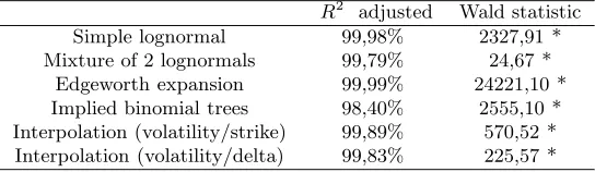
on 95% and 99% bands are respectively 5.99 and 9.21. A statistic higher (lower) than 5.99 implies the rejection (acceptance) of the null at a 5% confidence level. The results are presented in table (2):
Not surprisingly, the coefficients of determination are very close to 100% and the regression parametersα0and
α1 are very close to respectively 0 and 1. Nevertheless,
the Wald test indicates that the null assumption is rejected for all the regressions and consequently, any of the six estimation methods provides satisfactory results from a statistical point of view.
All in all, we can say that non-parametric methods perform better than parametric and semi parametric methods. This result is not, though, confirmed by statistical tests. Naturally, this leads us to consider al-ternative comparison tools. In the following, I will focus on the RNDs themselves and study their profiles, which would constitute an important source of exploitable information.
3.2
Implied RND function vs. true density
function
The RND is not the true probability density. Whereas the former is inferred from quoted option prices, the latter is not available and should be estimated from observable time series of the underlying asset. The difference be-tween the two distributions arises from the presence of risk aversion: indeed, the RND can be interpreted as the market’s aggregate beliefs regarding future states of the world and consequently, incorporates investor’s attitude toward risk. The RND would be equivalent to the true market density only if there is no aggregate risk in the market or assuming risk neutrality.
Working with simulated data overcomes this problem: not only the actual density is available and directly de-rived from various simulated scenarios of the underly-ing asset, but also the RND integrates no formulation
about risk aversion since it is estimated from simulated option data and not from real option data. Thus, the RND should be exactly equal to the true density func-tion. Based on this assertion, one possibility of compar-ing RND estimation methods raises: which one would provide the most accurate estimation of the ‘real’ density function?
To answer this question, I estimate first the true den-sityqtruefrom the 5000 simulated underlying pricesF in
theCase Band second, apply separately each of the six
estimation methods on option prices to derive the RND qRN D .The estimation ofqtrue is carried out using
Ker-nel estimator K(u) to obtain a sufficiently smooth and continuous density function:
qtrue(F) =
1 N h
N
X
i=1
K(F−Fi h )
WhereR
K(u)d(u) = 1 to ensureqtrueto be a probability
density function and h is the bandwidth of the Kernel estimator. I choose to work with the Gaussian Kernel which is the most commonly used.
Crucial for the Kernel estimation is the choice of the lo-cal bandwidth; a too small one will lead to an erratic distribution whereas a too large one will smooth away important details in the distribution. For this, I follow [?] who proposes an optimal value for the bandwidthhopt:
hopt= 0.9N
−1
5A
WhereA= min(σ, iqr/1,34),iqr being the interquartile range.
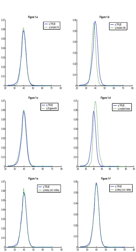
Figures (1a-f) display estimated RNDs and true densities for each of the estimation methods4.
The graphics above underscore the following observa-tions:
– All RNDs underestimate the left tail of the true den-sity. Indeed, the left true density tail lies systemat-ically below its RND counterpart. In a real world, this report would be interpreted so as the market does not expect any crash in the underlying asset and therefore assigns low probability to the occur-rence of this event.
– Interpolation methods are the best to fit correctly the true density and the two densities are almost superposed.
– On the RND provided by interpolation method in a space (volatility / strike), some erratic movements are observable around the mode. Nervertheless, they
4
Over a list of 500 observations of RNDs and true densities, those represented in the figure (1) correspond to the 131e
observation. Proceedings of the World Congress on Engineering 2007 Vol II
do not appear if the interpolation is performed in the (volatility / delta) space. So, we can say that moving from a (volatility / strike) space towards a (volatility / delta) space makes the RND smoother and avoids the appearance of abrupt jumps in the probabilities. This result is not surprising since the objective to move from the first to the second space is indeed to prevent such distortions.
– The implied binomial tree method and the mixture of lognormals provide completely shifted RNDs com-pared to the true density. This indicates that the mean of the distribution is wrongly estimated by these two techniques.
The question of whether visible differences between the two densities are statistically significant needs to be addressed by using non parametric goodness of fit tests. I consider two goodness-of-fit tests: the two-sample Kolmogorov-Smirnov and the two-two-sample Cramr-von Mises. These tests compare the cumulative distri-bution functions rather than the probability distridistri-bution functions. More concretely, the two-sample Kolmogorov-Smirnov test (KS) is based on the maximum distance be-tween two curves. It takes into account the whole of dis-tribution’s quantiles to test the assumption H0:Qtrue=
QRN D, whereQis the cumulative distribution function:
Q=R
q(u)du. This is based on the following test statis-tic:
D= sup
F
h
Qtrue(F)−QRN D(F)
i
The two-sample Cramr-von Mises (CvM) statistic mea-sures the quadratic deviations between two curves:
ω2= 1 4
N
X
i=1
Qtrue(Fi)−QRN D(Fi)
2
Table (3) displays the reject percentage of the null at 5% and 10% levels for each of the estimation methods:
It is clear from the results in Table (3) that the two tests do not provide exactly the same results and the CvM test seems to be more ‘conciliate’ by rejecting the null as-sumption in only two cases (the implied tree method and the interpolation in a (volatility / strike) space method). This obvious lack of precision leads us to prefer the KS test which, by taking the maximum distance between the two densities, gives more information about extreme de-viations. This test indicates that Edgeworth expansion method provides incontestably the best statistical perfor-mance with an acceptance rate of 100%: for each of the 500 observations, the density estimated using this method agrees with the true density with a difference statistically non significant. Moreover, the choice of an interpolation
space proves to be very important insofar as switching between the two spaces improves appreciably the results (for example, the rejection rate decreases from 12.4% to 1.8% at 5% level by moving from the (volatility / strike) space to the (volatility / delta) space). The poor perfor-mance of the implied binomial tree method is confirmed and the null assumption is rejected into almost half of the cases regardless of the confidence band.
3.3
Testing the forecasting performance of
RNDs
Forecast evaluation consists in using the true density as a point of reference to rank the RND estimation tech-niques relative to their ability to well approximate the true density. In this way, [10] use the Probability Inte-gral Transform (PIT) approach, initially proposed by [8], as an appropriate mean of evaluation of density forecast. The PIT score is defined as:
zi,τ =
Z St+τ
−∞
qi(u)du
=Qi(St+τ)
If forecasts and true densities coincide, then the sequence of PITszi of the realized outcomesSt+τ observed at
ma-turity is independently and identically distributed (i.i.d) with uniform distribution:
{zi}ni=1
iid
∼U(0,1)
The main power of the PIT approach is that it holds regardless of the particular method followed to produce the density forecasts, and therefore, can be used for all the RND estimation techniques. For practical applica-tions, testing whether the PIT series is i.i.dU(0,1) can be achieved by using simple visual tools such as histograms or by carrying out goodness-of-fit tests.
Before starting the estimation, we need to put the prob-lem in context by presenting the manner by which the se-quence of the PITs is obtained. At every 21stobservation
along the sequence of realization {St}11000t=500 of Case A,
one PIT is calculated for each of the six estimated RNDs. The forecast procedure starts at the first observation of St(i.e. at the 500eobservation) and the PIT is obtained
by calculating the cumulative probability corresponding to the realization observed 21 days later:
z500=Q500(S521)
Then, I move 21 days forward and calculate the second PIT staring at t = 521 to obtain the PIT for the real-ization 21 days later. This procedure is repeated a total
of 500 times in order to generate 500 z-values for each of the six RND estimation methods. As it was previously mentioned, the sequence{zi}500i=1 should be i.i.dU(0,1) if
the RND provide good forecast of the true density. Because of their ease of interpretation, histograms of the z-series are used to verify the requirement that z is uni-form over the interval [0,1]5. Figure (2) provides 15
bins-histograms relative to each of the RND estimation meth-ods. If the density forecast is correctly calibrated then, each of the histograms should be roughly flat and a ran-dom of 10% of the 15 bars should fall outside the two horizontal lines delimiting the 90% confidence interval.
It appears rather clearly that any of the estimation tech-niques provides a good forecast of the true density since systematic deviations from uniformity are observed in the histograms. In the best of cases, only 8 of the 15 bars are inside the confidence interval (case of the mixture of log-normals, the Edgeworth expansion and the interpolation in space (volatility / delta) method). The most signif-icant violations are in particular observable around the tails of the distribution: indeed, it appears that there are many observations in the two extremes which sug-gest that RNDs have tails which are too thin. Except for the implied tree method, the RND tails tend to be above their true density’s counterparts which means that the RND assigns more probability to extreme outcomes than it is observable on the effective realizations. These U-shaped histograms can also be explained by the fact that the forecast provides a too narrow variance of the true density, resulting in a shaped distribution with thin tails.
The comparison based on the uniform distribution could be inappropriate for small sample size which is the case here. Moreover, the fact that the comparison interval is limited between 0 and 1 may make the results hard to interpret. For these reasons, [9] suggests applying a transformation to normality to the PIT series:
xi,τ =N
−1(z
i,τ) =N
−1
Qi(St+τ)
If the sequence ofziis iidU(0,1), then the sequence ofxi
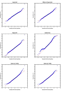
must be iid according to a standard normal distribution. The normal transformation allows the application of sev-eral comparison techniques and tests. Among these tech-niques, the well-known QQ-plot of the normal transform variables, which displays a quantile-quantile plot of the sample quantiles of xi versus theoretical quantiles from
normal distribution. If the distribution of xi is normal,
the plot will be close to line. Figure (3) displays these plots:
We can see that the RND predicts very well the body of the true density but much less its tails. As stated
5
The assessment of the i.i.d condition can be achieved by plot-ting correlograms of (z−E(z)) and powers of it.
previously, the RND underestimates the right tail of the true density and the empirical right-hand quantiles ofxi
are systematically above those of the standard normal distribution. However, concerning the left tail, the re-sults differ from those obtained from the histogram anal-ysis: the parametric methods (the simple lognormal, the mixture of lognormals and the Edgeworth expansion) overestimate the left tail of the true density (the em-pirical quantiles being above those of the standard nor-mal distribution) and the non-parametric methods (Smile interpolation-based methods) underestimate the left tail of the true density (empirical quantiles being below those of the standard normal distribution). In terms of absolute performance, it appears that the Edgeworth RND pro-vides the better forecast since it deviates rather slightly from the true density on the tails.
All RNDs, except the implied binomial tree RND, present the same profile for the body of the distribution and differ on the tails. Therefore, it becomes legitimate to focus on the extreme probabilities and the discrepancies between the true density and the RND around the tails can be studied more formally using the so-called scoring rule. The idea consists in defining a generic interval associated with the extreme quantiles{pl, pu}and a binary variable
Btwhich takes the value of 1 if the true realization of the
underlying falls into this interval and 0 otherwise:
Bt,τ=
(
1 if St+τ ∈ {pl;pu}
0 otherwise
The interval forecast is correctly calibrated if the ex-pected outcome of the underlying asset inside the pre-specified interval is equal to the probability defined by the extreme quantiles: E(Bt,h) =pu−pl. Table (4)
re-ports the results according to the estimation technique:
More than a confirmation of the bad forecast performance in the tails of the RNDs, already observed on the his-tograms of the figure (1), these results permit to quantify the magnitude of these violations. It appears that, even if all techniques fail to assess correctly the tails, some do better job than others. In fact, the Edgeworth expansion seems to be the best with the lowest score either in the left tail or in the right tail; comes then the mixture of lognor-mals, the two non-parametric interpolation methods, the simple lognormal and finally the implied binomial trees which should be rejected without any regret.
4
Conclusion
This paper sets out to examine the empirical performance of six RND estimation techniques using three different comparison tools (the pricing errors, the true density ap-proximation and the forecast performance). The main result that arises is that the choice of the suitable RND es-timation technique depends on the purpose of the study:
if the RND is used within an option pricing framework, non parametric techniques would be the best; they in-deed provide the lowest evaluation errors. This is rather surprising because for parametric approaches, the distri-bution is obtained directly by minimising the pricing er-rors whereas in the non parametric methods, the implied volatilities, and not the option prices, are approximated. However, if the purpose is to study market expectations, the Edgeworth expansion technique should be used with caution since it approximates very well the body of the true density and performs relatively not badly around the tails.
This result may be interesting for academics and prac-titioners concerned by investigating market expectations implicit in option prices. Future researches may use real data to see whether the most suitable technique depends on market characteristics not.
References
[1] B. Silverman,Density Estimation for Statistics and Data Analysis, Chapman and Hall Publisher, 1986.
[2] S. A. Syrdal, A study of Implied Risk-Neutral Density Functions in the Norwegian Option Mar-ket,Journal of Finance, 2002
[3] S. Markose, A. Alentorn, “Bank of England,” The Generalized Extreme Value (GEV) Distribution Im-plied Tail Index and Option Pricing, 2005
[4] R. R. Bliss, N. Panigirtzoglou, “Bank of England,” Testing the Stability of Implied Probability Density Functions, 2000
[5] M. Andersson and M. Lomakka, “Riksbank Research Paper Series No. 1,” Evaluating Implied RNDs by Some New Confidence Interval Estimation Tech-niques, 2001
[6] N. Cooper, “Bank of England,”Testing Techniques for Estimating Implied RNDs from the Prices of Eu-ropean Style Options, 1999
[7] J. C. Jackwerth, “Review of Financial Studies,” covering Risk Aversion from Option Prices and Re-alized Returns, V13, N2, pp. 433-45
[8] M. Rosenblatt, “Annals of Mathematical Statistics,” Remarks on a multivariate transformation, V23, pp. 470-72
[9] J. Berkowitz, “Journal of Business and Economic Statistics,” Testing density forecasts, with applica-tions to risk management, V19, pp. 465-74
[10] F. X. Diebold, T. A. Gunther, A. S. Tay, “Interna-tional Economic Review,” Evaluating density fore-casts with applications to financial risk management, V39, pp. 863-83
RMSE×10−3
RRMSE×10−3
Simple lognormal 1.94 (0.97) 6.02 (7.95) Mixture of 2 lognormals 9.99 (49.75) 3.55 (7.73) Edgeworth expansion 1.22 (0.25) 1.33 (3.57) Implied binomial trees 99.78 (49.96) 7.56 (26.92) Interpolation (volatility/strike) 0.59 (0.84) 0.62 (8.09)
[image:7.612.305.577.197.276.2]Interpolation (volatility/delta) 0.67 (0.85) 0.63 (0.81)
Table 1: RMSE and RRMSE Means and standard devia-tions (between brackets) for each of the estimation meth-ods
R2
adjusted Wald statistic Simple lognormal 99,98% 2327,91 * Mixture of 2 lognormals 99,79% 24,67 *
Edgeworth expansion 99,99% 24221,10 * Implied binomial trees 98,40% 2555,10 * Interpolation (volatility/strike) 99,89% 570,52 *
[image:7.612.303.583.349.451.2]Interpolation (volatility/delta) 99,83% 225,57 *
Table 2: Coefficients of determination, regression param-eters and Wald test results. * indicates the significance at 5% and 1% levels.
Test de KS Test de CvM H0:Qtrue=QRN D Rejet H0 Rejet H0
5% 10% 5% 10%
[image:7.612.306.609.574.652.2]Simple lognormal 1.6% 6.6% 0% 0% Mixture of 2 lognormals 10% 10.2% 0% 0% Edgeworth expansion 0% 0% 0% 0% Implied binomila trees 44.2% 45.6% 32.2% 35% Interpolation (volatility/strike) 12.4% 14% 3.4% 3.4% Interpolation (volatility/delta) 1.8% 3.4% 0% 0%
Table 3: Kolmogorov-Smirnov and Cramr-von Mises tests for the goodness of fit between the RND and the estimated true density. Note: ‘rejectH0’ is the
percent-age of rejection of the null assumption at 5% and 10% levels. The critical values of the KS test at 5% and 10% levels are respectively 0.0270 and 0.0243; those of the CvM test are respectively equal to 0.4614 and 0.3473.
{pl;pu}={0; 0.05} {pl;pu}={0.95; 1}
Simple lognormal 0.1 0.04 Mixture of 2 lognormals 0.076 0.06 Edgeworth expansion 0.068 0.052 Implied binomial trees 0.02 0.094 Interpolation (volatility/strike) 0.08 0.074 Interpolation (volatility/delta) 0.076 0.074
Table 4: Score tail tests performed separately on the left and the right tails of the forecast density for each of the RND estimation methods.
20 30 40 50 60 70 80 0
[image:8.612.55.284.122.546.2]0.01 0.02 0.03 0.04 0.05 0.06 0.07
Figure 1-a
q TRUE q simple LN
20 30 40 50 60 70 80 0
0.01 0.02 0.03 0.04 0.05 0.06
Figure 1-b
q TRUE q double LNs
20 30 40 50 60 70 80 0
0.01 0.02 0.03 0.04 0.05 0.06 0.07
Figure 1-c
q TRUE q Edgeworth
20 30 40 50 60 70 80 90 0
0.01 0.02 0.03 0.04 0.05 0.06 0.07
Figure 1-d
q TRUE q implied trees
20 30 40 50 60 70 80 0
0.01 0.02 0.03 0.04 0.05 0.06
0.07 Figure 1-e
q TRUE q interp (vol / strike)
20 30 40 50 60 70 80 0
0.01 0.02 0.03 0.04 0.05
0.06 Figure 1-f
q TRUE q interp (vol / delta)
Figure 1: True probability density and RND for each estimation technique.
0 0.10.20.30.4 0.5 0.6 0.7 0.8 0.9 1 0
10 20 30 40 50 60
Lognormal
00.10.20.30.4 0.5 0.6 0.7 0.8 0.9 1 0
10 20 30 40 50
Mixture of Lognormals
0 0.10.20.30.4 0.5 0.6 0.7 0.8 0.9 1 0
10 20 30 40 50
Edgeworth
0 0.10.20.30.4 0.5 0.6 0.7 0.8 0.9 1 0
10 20 30 40 50 60 70 80
Implied trees
00.10.20.30.4 0.5 0.6 0.7 0.8 0.9 1 0
10 20 30 40 50 60
Interp (vol / strike)
0 0.10.20.30.4 0.5 0.6 0.7 0.8 0.9 1 0
10 20 30 40 50
[image:8.612.307.543.179.497.2]interp (vol / delta)
Figure 2: Histograms of Probability Integral Transforms with 90% confidence bands for each of the RND estima-tion methods.
-4 -3 -2 -1 0 1 2 3 4 -6
-4 -2 0 2 4 6
Standard Normal Quantiles
Q
u
a
n
ti
le
s
o
f
x
Lognormal
-4 -3 -2 -1 0 1 2 3 4 -6
-4 -2 0 2 4 6
Standard Normal Quantiles
Q
u
a
n
ti
le
s
o
f
x
Mixture of lognormals
-4 -3 -2 -1 0 1 2 3 4 -4
-3 -2 -1 0 1 2 3 4 5 6
Standard Normal Quantiles
Q
u
a
n
ti
le
s
o
f
x
Edgeworth
-4 -3 -2 -1 0 1 2 3 4 -4
-3 -2 -1 0 1 2 3 4
Standard Normal Quantiles
Q
u
a
n
ti
le
s
o
f
x
Implied trees
-4 -3 -2 -1 0 1 2 3 4 -4
-3 -2 -1 0 1 2 3 4 5 6
Standard Normal Quantiles
Q
u
a
n
ti
le
s
o
f
x
Interp (vol / strike)
-4 -3 -2 -1 0 1 2 3 4 -4
-3 -2 -1 0 1 2 3 4 5 6
Standard Normal Quantiles
Q
u
a
n
ti
le
s
o
f
x
[image:9.612.47.303.150.528.2]Interp (vol / delta)
Figure 3: QQ-plot of Normal Transforms of the Probabil-ity Integral Transforms for each of the RND estimation methods.