Online Full Text

Abstract—This paper studies the simultaneous scheduling of landside container handling operations in a container terminal. Issues addressed include scheduling the sequence of loading (unloading) of containers to (from) the vessels from (to) the quayside, assigning trucks to transport containers between quayside and yard side, and scheduling operations of yard cranes in different yard zones. A mathematical model describing the characteristics of the problem is developed. The objective is to minimize the total completion time for handling all the containers under consideration in the terminal. As optimizing the landside container handling operations in a terminal is known to be NP-hard, a new genetic algorithm with the selection process based on the principle of simulated annealing is developed in this paper to solve the problem. Comparison of the respective results obtained by using the proposed genetic algorithm, the canonical genetic algorithm and the simulated annealing algorithm clearly shows that the total completion times obtained by the proposed algorithm are 12%-18% shorter than that obtained by GA and SA, and the computing times of GA-SA are only 50% of that of GA. The proposed genetic algorithm is indeed superior to the other two algorithms.

Index Terms—container handling scheduling, genetic algorithm (GA), simulated annealing (SA), truck assignment, yard crane scheduling

I. INTRODUCTION

Driven by the remarkable growth in international trade, sea transport plays an important role around the world. The demand of container marine transportation has significantly increased in recent decades. As a substantial proportion of international cargo is transported in containers through major container terminals, enhancement of the competitiveness of container terminals has become urgent, especially in Europe and Asia. A reasonable time for handling containers in a container terminal is crucial to improve customer service performance. In most terminals, a large portion of container handling time is spent on container discharging and loading. In order to shorten the total handling time of containers, the scheduling of all the container handling operations in the terminal should be studied carefully.

Sequencing container handling jobs in a container terminal is a complicated problem, for all terminal resource, such as mobile trucks, yard cranes and quay cranes, must cooperate to offer handling services to thousands of containers each day. Besides, both the arrival times of vessels and the number of

K. L. Mak is Professor in the Department of Industrial and Manufacturing Systems Engineering, The University of Hong Kong. (Tel: (852) 28592582; E-mail: [email protected]).

L. Zhang is an Mphil student in the Department of Industrial and Manufacturing Systems Engineering, The University of Hong Kong. (E-mail: [email protected]).

containers to be handled affect the total completion time for handling containers, and both are difficult to predetermine.

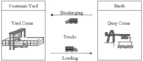
Fig. 1.1 Typical container handling process in a container terminal

A typical container handling process in a container terminal is shown in Fig. 1.1. When a vessel carrying containers arrives at a container terminal, multiple quay cranes are assigned for discharging job. And mobile trucks move from the landside of the terminal to the quayside to transport the containers to the yard side for storage. Meanwhile, in each yard zone, the assigned yard cranes are gathered to discharge containers from mobile trucks. When the discharging job finishes, the trucks, yard cranes and quay cranes are released and are ready to be assigned to the next job. This is the import process. The export process is reversed.

Due to the complicated import/export container handling processes, the sequence of the terminal resources would change as their responding locations change. Researchers studied container terminal scheduling from many aspects. Zhang (2005) [1], Kozan (1999) [2] and Mattfeld et al. (2003) [3] studied truck scheduling problem in container terminals using Genetic Algorithm. Zeng (2009) [4], Zhang (2002) [5], Kim et al. (2003) [6], Kim et al. (1999) [7] and Li et al. (2008) [8] have spent much effort on yard crane scheduling problem. They also used Genetic Algorithm to solve the problem. However, these studies only schedule one kind of terminal resource. For example, the truck scheduling problem or the yard crane scheduling problem is studied separately. However, in a real container terminal, resources are working together, not separately. Thus, integrated scheduling of multiple resources is essential to improve the efficiency of container handling. In this paper, trucks, yard cranes, and loading (unloading) of containers to (from) the vessels are scheduled simultaneously to get the minimum completion time for handling all the containers under consideration in a container terminal. In the analysis, a handling job refers to the movement of a container from the vessel to the yard side for an import container or from the yard side to the vessel for an export container.

Simultaneous Scheduling of Import and Export

Containers Handling in Container Terminals

Ng (2005) [9,10] and Bish (2003) [11] pointed out that optimizing quay crane scheduling, truck assignment and yard crane scheduling is a NP-hard problem which can only be solved by using heuristic algorithms. Indeed, genetic algorithm (GA) has received wide adoption because of its user friendliness and its ability to search in the global solution space. However, the problem of premature convergence of the search process often needs to be addressed. In this research, a new genetic algorithm with the selection process based on the principle of simulated annealing (GA-SA) is developed as an effective and efficient means to solve the problem.

This paper is organized as follows. Section 2 presents the mathematical model describing the scheduling problem for finding the minimum total completion time for handling all the containers under consideration. Section 3 presents the new genetic algorithm. Section 4 presents the evaluation of the performance of the proposed algorithm by comparing the algorithm with canonical GA and SA using numerical examples, and Section 5 presents the conclusion.

II. MATHEMATICAL MODEL

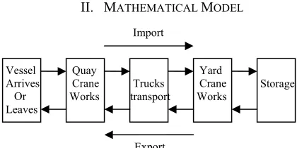
Fig. 2.1 Container terminal operation process

Fig. 2.1 presents the process of handling import and export containers within a container terminal. Generally, there are a number of yard cranes working at the same time in various predetermined yard zones discharging containers from truck to storage location or loading containers from storage location onto trucks. Although in practice, each yard zone always has more than one yard cranes, as yard crane interference would not be considered in this research, it is assumed that there is only one yard crane working in each yard zone. Transporting containers between quayside and yard side is handled by highly mobile trucks. In addition, a vessel is usually served by several quay cranes working together. However, this paper assumes that detailed working sequence of these quay cranes is not a major concern and there is sufficient quay crane capacity in the terminal.

In the proposed model, suppose there are N jobs to be handled. Each job needs one quay crane, one truck and one yard crane. The relationships of them are shown in Fig 2.2.

For an export job, container iis firstly loaded onto trucks by yard cranel in the yard side. Trucksthen transports container ito the quayside to be loaded onto a vessel by a quay crane. Therefore, the completion time of an export job can be given by XQ_i+hq where _XQiis the starting time of the quay crane servicing containeri, andhqis the quay crane’s handling time which is a predetermined constant. Similarly, for an import job, the handling sequence is

reversed. And the completion time is given by XY_i +hy where_XYiis the starting time of the yard crane servicing jobi, andhy is the yard crane handling time which is also a predetermined constant.

∙

∙

∙

Fig. 2.2 The relationship of job, truck, YC and QC

Parameters and Variables:

The following notations are used in the proposed integer program model:

N : the number of containers to be loaded (unloaded) to (from) vessels.

tr

K : the number of trucks in the container terminal K_yc: the number of yard cranes in the terminal CTi: the completion time of handling container i XTi: the ready time of container i

XQi: the quay crane starting time for container i XYi: the yard crane starting time for container i WTi: the ready time of the truck which transports container i

1

WL i: the travelling time for the truck to move to the pick up location of container i

2

WL i: the travelling time for the truck to transport container ifrom the pick up location to the drop off location

YTi: the ready time of the yard crane for handling container i

YLi: the travelling time for the yard crane to travel from the pick up location to the drop off location of container i

hq: handling time of quay crane hy: handling time of yard crane

pxi: truck pick up location x of container i

Job N

QC N Truck N YC N Job 1

QC 1 Truck 1 YC 1

Vessel Arrives Or Leaves

Quay Crane Works

Trucks transport

Yard Crane Works Import

Export

pyi: truck pick up location y of container i dxi: truck drop off location x of container i dyi: truck drop off location y of container i v: travelling speed of truck

Yij: 1, container is handled before container _0, i _Otherwise j



U_ik: 1, truck is assigned to transport container

0, Otherwise

k i

 



V_il: 1, yard crane is assigned to handle container

0, Otherwise

l i

 



Opi: 1, container is for export_{0, container is for importi}i



Objective: Min

1,2,...,max i

i N

CT =

where

1 , 1, 2,...,

CT_i =Op_ig_XQ hq_i+ _+ −_ Op_{i }  g XY_i+hy_ i= N (1)

{

}

max , , 1 2

1,2,...,

XQ_i Op_i XT YT YL WT WL_{i i i i i} hy WL _i

i N         = + + + + = g

{

}

1 max , 1

1,2,...,

Op_i XT WT WL_{i i i}

i N        _{  }  _{ } + − + = (2)

{

}

max , , 1

1,2,...,

XY_i Op_i XT YT YL WT WL_{i i i i i}

i N         = + + = g

{

}

1 max max , 1 2 , 1,2,..., 1,2,...,

Op_i XT WT WL_{i i i} hq WL _iYT YL_{i i}

i N i N

 _{ }               + − + + + + = = (3) 1 1

WT_i+ =Op_ig_XQ hq_i+ _+ −_ Op_{i }  g XY_i+hy_ (4)

1

YT_i+ = XY_i+hy (5)

(

) (

)

1 _{1 1}

WL_i dx px_i dy py_i v

i i

= ₋ − + ₋ − (6)

(

) (

)

2

WL _i = px_i−dx_i + py_i−dy_i v (7)

Subject to:

, 0

XQ_i >XT Op_{i i} = (8)

, 1

XY_i >XT Op_{i i} = (9)

2 , 0

XY_i >XT_i +hq+WL _i Op_i = (10)

2 , 1

XQ_i >XT_i +hy+WL _i Op_i = (11)

(

)

( )

(

)

Op XT_i Op_i XQ M Y_ij Op_j XT Op_j XQ

i+ − i≤ − + j+ − j

g g g g

(12) 1

Y_ij+Y_ji = (13)

1 1

Ktr

s= Uis =

∑ (14)

1 1

K yc

l= Vil =

∑ (15)

{ }

, , 1, 0

1, 2,..., ; 1, 2,..., ; 1, 2,..., Y_ij U_is V

il

i N s K_tr l _{K yc}

∈

= = = (16)

The objective of the scheduling problem is to minimize the total completion time of all jobs to be handled in the terminal. Equation (1) explains the calculation of the completion time of each job. Equations (2) and (3) explain the calculation of the starting time of quay cranes and yard cranes of each job. Equations (4) and (5) explain the calculation of the ready time of trucks and yard cranes of each job. Equations (6) and (7) the calculation of the travelling time between container pick up location and drop off location of each job. Constraint (8) ensures that for import jobs, containers can be handled by quay cranes only after their ready time. Constraint (9) ensures that for export jobs, containers can be handled by yard crane only after their ready time. Constraint (10) ensures that for import job, containers can be handled by yard crane only after their arrival at yard blocks. Constraint (11) ensures that for export job, containers can be handled by quay crane only after their arrival at quayside. Constraint (12) ensures that if container iis handled before container j, Y_ij =1. Constraint (13) indicates that container iis either handled before or after container j . Constraints (14) and (15) ensure that each container is handled and transported by only one yard crane and one truck. Constraint (16) specifies the range of each decision variable.

III. THEPROPOSEDALGORITHM

A. Genetic Algorithm - Simulated Annealing (GA-SA) Container terminal operation scheduling problem is NP-hard, and heuristic algorithm must be used to get an optimal solution of the proposed mathematical model in reasonable computing time. However, in canonical GA, individuals have a high probability to change with uncertainty in computing process, and superior individual’s priority for survival is not dominant. In this case, canonical GA always has the problem of premature convergence, which leads a long computing time. Thus, GA-SA has been proposed to solve the problem.

The general steps of the proposed algorithm are as follows: Step 1:

Let : 0k = , and generate the initial temperaturet_k :=t₀. And randomly generate the initial populationP₀.

Step 2:

Pick up the individual with the largest fitness value, and put it directly into the next generation.

Step 3:

Step 4:

According to the crossover probability, select parent individuals to generate new individuals to form populationC_k.

Step 5:

Using mutation operator to populate C_k , and get populationM_k.

Step 6:

1: ( )

k k

t ₊ =d t , :k = +k 1,P_k =M_k . Repeat Step 2 to Step 6, untiltk <ε.

B. Solution Representation

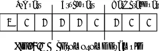
The goal of this research is to schedule trucks, yard cranes and loading/unloading jobs to/from vessels simultaneously in a container terminal. Thus, integer strings are used as chromosomes to represent these sequences. LetN be the amount of the jobs to be handled, and the length of the chromosome is 3N , which is the combination of three parts: first Nnumbers present the sequence of loading/unloading jobs; the next N numbers present the sequence of trucks assigned to the job; the lastNnumbers present the sequence of yard cranes assigned to the job.

Fig. 3.1 A chromosome example

Fig. 3.1 is an example of the representation of a chromosome. Here, N =3, and the chromosome length equals to 9. Also, let 2,K 2

tr yc

K = = . The numbers in Job part are “3-1-2”. It means container 3 must be handled first, then container 1, and container 2 is the last. In Truck part the numbers are “2-2-1”. It means that container 3 and container 1 would be serviced by truck 2, and container 2 by truck 2. Similarly, the numbers in Yard crane part are “2-1-1”, so yard crane 2 is assigned to handle container 3, and yard crane 1 for container 1 and container 2.

C. Simulated Annealing Selection Operator

The selection operator used in the proposed algorithm is based on the principle of simulated annealing algorithm, which is different from the traditional roulette selection operation. The probability of survival of the ith individual in each iteration can be calculated by

( ) ( )

( ) min( ) min

exp( ) exp( )

( ) i j

i

k _{j k} k

f b f k

f b f k

t _{b P} t

P b − − ∑ − −

∈ =

(3.1) where, ( )_{f bi} is the objective function value of solution _bi,

( ) min

f k is the minimal objective value of populationP_k, and

k

t is the simulated annealing temperature which goes down to

zero.

The initial temperature t₀is an important parameter in the algorithm. If the initial temperature is too high, it would cause the number of iterations increasing and the computing time would be rather long. However, if the initial temperature is too low, it would lead to process converges to the local optimal. Hence, in the proposed algorithm, the initial temperature is computed by formulation (3.2).

0

t = ∆K (3.2) where, K is a given constant. Usually K =2, 5, 10,L according to different problems, and

0 0

max{1 / ( )f b_i b P_i } min{1 / ( )f b_i b P_i }

∆ = ∈ − ∈ (3.3) To ensure fast convergence, the value of t_kin equation

(3.1) can be set to decrease according to either one of the following equations as k increases

0

k

k

t =M ⋅t , k ₀

k

t =M ⋅t ,k=1, 2,K (3.4) 0

ln( 1)

k

k

t = _t + , k=1, 2,K (3.5) M is a randomly chosen parameter which controls the decreasing process oft_k, and 0<M <1.

In the proposed algorithm, when the temperature is high, the survival probabilities of different individuals are close to each other. Hence, individuals’ diversity can be kept. As the temperature decreases, the difference of individuals’ fitness would be enlarged because the scaling function of the Simulated Annealing operator strengthens. It means that, superior individuals are much easier to survive. In this case, the problem of canonical GA can be effectively solved. And in the final stage of the computing process, this selection policy can speed up the convergence of the algorithm.

D. Crossover and Mutation Operations

Crossover and mutation processes are also two key features besides selection. The two operations can offer individual diversity during the searching process. And they are controlled by predetermined parameters, called crossover rate and mutation rate. In the proposed algorithm, One-point Crossover and Simple Mutation are employed.

IV. COMPUTATIONALRESULTS

The proposed Genetic Algorithm with Simulated Annealing Selection (GA-SA) described in the last section will be tested. The proposed algorithm is firstly compared with the canonical GA and the canonical SA using small size examples, and then using large size examples.

In this research, the problem set is decided by (N,

tr

K , yc

K ). N is the number of the loading/unloading jobs to/from vessels, K_tris the number of mobile trucks, and

yc

K is the number of yard cranes. These numbers are predetermined in the program. Other parameters of the problem are needed to be determined as follows:

,

hy the handling time of a yard crane = 4; hq, the handling time of a quay crane = 2;

v, the travelling speed of a truck = 5;

_

POP SIZE, the population size = 200; _

cross rate, the crossover rate = 0.7;

_

mutation rate, the mutation rate = 0.1; M , the parameter used to calculate t_k = 0.07;

K, the parameter used to calculate t₀= 2.

The ready times and locations of containers, trucks and yard cranes are also randomly generated.

A. Small size examples

The performances of GA-SA, canonical GA and the SA are compared by using small size examples. The computer uses Inter Penium 2.4GHz and 512MB RAM. The results are shown in Table 4.1. In the Table, TCTis the total completion time and CT is the computing time.

Algorithm _{N K}

tr Kyc TCT/ min CT/ sec GA-SA 5 3 4 64.363541 <1

10 3 4 114.806728 <1 GA 5 3 4 64.300680 <1 10 3 4 134.162253 <1 SA 5 3 4 65.002560 6

10 3 4 137.184561 10 Table 4.1 Results of solving small size problems

It can be seen that the number of trucks and yard cranes are the same for these problems, i.e., K_tr =3,K_yc =4. When

5

N = , the three algorithms have similar optimal total completion times. However, when N =10 , the total completion time of GA-SA is 17% shorter than that of GA and 20% shorter than that of SA. It can also be seen that GA-SA and GA require similar computing time while SA requires longer processing time to achieve the results.

B. Large size examples

The results of the three algorithms for large size problems are shown in Table 4.2.

Algorithm _{N K}

tr Kyc TCT/min CT/sec

GA-SA 20 30 10 6 124.852164 179.543070 2 3 60 339.379189 8

GA 20 30 10 6 141.404902 206.061680 3 6

60 414.662828 17

SA 20 30 10 6 141.831165 201.565223 5 41 60 420.753142 >500 Table 4.2 Results of solving large size problems It can be seen that the total completion times obtained by GA-SA are 12%-18% shorter than that obtained by GA and SA. Besides, the computing times of GA-SA are only 50% of that of GA, and SA’s computing times are much longer.

C. Parameter analysis

M and K are two parameters which can control the temperature according to formulation (3.2) and (3.4). Table 4.3 shows the calculating results whenM andK equal to

different values. HereN =60,K_tr =10,K_yc =6. M K TCT/ min 0.07 2 343.806728 0.07 5 364.162253 0.4 2 357.184561 0.4 5 368.372596 Table 4.3 TCT with different M andK

Fig. 4.1 Convergence comparison of different K , when 0.07

M =

Fig. 4.2 Convergence comparison of different K , when 0.4

M =

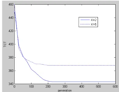
Fig. 4.1, 4.2 and Table 4.3 indicate that the searching process of the proposed algorithm converges faster whenM andK increase. However, as M and K grow, premature convergence may occur. Thus, appropriate value of parameters M and K are very important to the proposed algorithm, GA-SA.

D. Convergence analysis

Fig. 4.3 illustrates the convergence behavior of GA-SA and GA for the problem whenN =60,Ktr =10,Kyc =6. It can be seen from the figure that GA-SA converges slower than GA in the early stage of the computing process. However, it converges faster and generates better solution in the later generations than canonical GA.

Fig. 4.3 Convergence comparison of GA-SA and GA

V. CONCLUSION

This paper has studied the problem of scheduling the loading (unloading) of containers to (from) vessels, trucks and yard cranes simultaneously in a container terminal. The objective is to minimize the total completion time for handling the containers under consideration. A mathematical model has been proposed to highlight the characteristics of the scheduling problem. A new genetic algorithm with the selection process based on the principle of simulating annealing (GA-SA) has been developed to find optimal schedules for the problem. The performance of GS-SA has been evaluated by using a set of test problems. The computational results have shown that the total completion time for handling containers under consideration obtained by GA-SA is 12%-18% shorter than that of the canonical GA and the SA. Also, the computing time of GA-SA is much shorter than that of the other two approaches. Hence, the proposed algorithm is an effective and efficient means for simultaneous scheduling of container handling operations in container terminals.

REFERENCES

[1] Y. X. Zhang, “Scheduling Trucks in Port Container Terminal by a Genetic Algorithm”, Dept. of Industrial Manufacturing Systems Engineering, The University of Hong Kong, 2005.

[2] E. Kozan, P. Preston, “Genetic Algorithms to Scheduling Container Transfers at Multimodal Terminals”, Intl. Trans. in Op. Res. 6, 1999,

pp311-329.

[3] D. C. Mattfeld, H. Kopfer, “Terminal operations management in vehicle transshipment”, Transportation Research Part A 37, 2003,

pp435–452.

[4] Q. C. Zeng, Z. Z. Yang, “Integrating simulation and optimization to schedule loading operations in container Terminals”, Computers & Operations Research, Volume 36, Issue 6, 2009.

[5] C. Q. Zhang, Y. W. Wan, J. Y. Liu, R. J. Linn, “Dynamic crane deployment in container storage yards”, Transportation Research Part B 36, 2002, pp537–555.

[6] K. H. Kim, K. M. Lee, K. Hwang, “Sequencing delivery and receiving operations for yard cranes in port container terminals”, Int. J. Production Economics 84, 2003, pp283–292.

[7] K. Y. Kim, K. H. Kim, “A routing algorithm for a single straddle carrier to load export containers onto a containership”, Computers & Industrial Engineering 36, 1999, pp109-136.

[8] Li, W., Wu, Y., Petering, M.E.H., Goh, M., de Souza, R., “Discrete Time Model and Algorithms for Container Yard Crane Scheduling”,

European Journal of Operational Research, doi:

10.1016/j.ejor.2008.08.019.

[9] W. C. Ng, “Crane Scheduling in Container Terminal Yards with Inter-crane Interference”, European Journal of Operational Research 164, 2005, pp64–78.

[10] W. C. Ng, K. L. Mak, “Yard Crane Scheduling in Port Container Terminals”, Applied Mathematical Modelling 29, 2005, 263–276. [11] E. K. Bish, “A Multiple-crane-contained Scheduling Problem in a

Container Terminal”, European Journal of Operational Research 144,

2003, pp83–107.