Stability of a Numerical Discretisation Scheme
for the SIS Epidemic Model with a Delay
Ekkachai Kunnawuttipreechachan
∗Abstract—This paper deals with stability properties of the discrete numerical scheme for the SIS epidemic model with maturation delay. We provide the suffi-cient conditions of the numerical step-size for the nu-merical solutions to be asymptotically stable. These will be useful for choosing a suitable numerical step-size when we simulate problems with the provided numerical scheme.
Keywords: SIS epidemic model, delay differential equa-tions, discrete numerical scheme, asymptotic stability
1
Introduction
In this paper we aim to analyse a numerical scheme for a class of the SIS epidemic models. In a general SIS model, the population sizeN(t) is divided into two groups: I(t) the infected population size, andS(t) the susceptible pop-ulation size. Here we continue further the results from Cooke et al. [1], who have developed the SIS epidemic model with maturation delay:
I0(t) = µ(N(t)−I(t))I(t)
N(t)−(δ+ε+γ)I(t),
S0(t) = B¡N(t−τ)¢N(t−τ)e−δ1τ
−δS(t)−µSN(t()tI)(t)+γI(t), N0(t) = B¡N(t−τ)¢N(t−τ)e−δ1τ
−δN(t)−εI(t). (1)
HereB(N) is a birth rate function,ε≥0 is the disease in-duced death constant rate,γ≥0 is the recovery constant rate (i.e. 1/γ is the average infective time),µ >0 is the contact constant rate, δ is the death rate constant, and δ1 is the transfer rate constant for the life stage prior to the adult stage. The standard incidence function µI/N refers to the average number of adequate contacts with infectives of one susceptible per unit time. The delay τ is considered as the development or the maturation time.
In addition, model (1) is based as follows on the assump-tions by Cookeet al.[1]:
• the transmission of the disease occurs due to a con-tact between the susceptible class S(t) and the
in-∗Department of Mathematics, King Mongkut’s
Univer-sity of Technology North Bangkok (KMUTNB), 1518 Pibul-songkram Road, Bangkok, THAILAND 10800; Tel:+66(0)81-828-3100/Fax:+66(0)28-587-8258. Email: [email protected], or [email protected].
fective classI(t);
• there is no vertical transmission;
• the disease presents no immunity against reinfection, i.e., on recovery, an infective individual returns to the susceptible class.
Moreover, in Cookeet al.[1], they also identified the basic reproduction number
R0= µ
δ+ε+γ, (2)
which generates the average number of new infective indi-viduals produced by one infective during the mean death adjusted infective.
Many authors have studied dynamics of the system (1) by considering R0 as a parameter [1, 2, 3]. Cooke et
al.[1] showed the existence of the equilibria of (1). They proved that if R0 < 1, there exists a unique nontriv-ial equilibrium ( ¯I,S,¯ N¯) = (0,N¯0,N¯0), called
disease-free equilibrium, which is globally asymptotic stable (see
Cooke et al.[1], Theorems 4.2 and Theorem 4.3). When R0 >1, there also exists another nontrivial equilibrium ( ¯I,S,¯ N¯) = ( ¯I+,S¯+,N¯+) or, so called, endemic
equi-librium. Analysis of the system in this case becomes
harder. For the non-delay problem (τ = 0), Cooke et al. [1] showed that the reproduction numberR0 acts as
a sharp threshold. Their results show that, for
nonneg-ative solutions, when R0 < 1, the disease dies out, i.e.
I(t) → I¯0 = 0 as t → ∞. On the contrary, if R0 > 1 and I(0) > 0, then the disease remains endemic with I(t)→I¯+,S(t)→S¯+ andN(t)→N¯+ ast→ ∞.
Our approach in this paper is to study a special class of (1). Assume that the death rate in each stage prior to the adult stage is negligible compared with the death rate of the adult stage, then we can assumeδ1= 0. Using the birth rate function B(N(t)) = pe−aN(t). Hence (1) becomes
I0(t) = µ(N(t)−I(t))I(t)
N(t)−(δ+ε+γ)I(t),
S0(t) = pN(t−τ)e−aN(t−τ)
−δS(t)−µSN(t()tI)(t)+γI(t), N0(t) = pN(t−τ)e−aN(t−τ)−δN(t)−εI(t).
(3)
Like with the model (1), the dynamical behaviour of the SIS model (3) is still largely undetermined because there are many open problems which are still unsolved at present [2]. In this paper we provide alternatively a numerical scheme for (3). Our aim is to analyse fur-ther the dynamical properties of a numerical scheme for (3). The main objective in this study is to determine the asymptotic stability of the equilibria of the given numer-ical scheme and illustrate numernumer-ical solutions of (3). We obtain the sufficient conditions for the numerical step-size causing the numerical solutions are asymptotically stable.
This paper is organised as follows. In the next section we analyse the stability of (3). For any nonnegative so-lutions, our result in Theorem 2 shows conditions for the existence of the equilibria, which are called disease-free
equilibriumandendemic equilibrium. Most results for the
continuous system have already been studied, but we re-state some related results with our own proof in Theorem 3 and Theorem 4 for the stability of (3). Later, in Section 3, we describe our main problems for this paper. Here we develop the numerical scheme for (3), and then investi-gate the stability of the numerical solutions. Our main contributions are presented in Theorem 6 and Theorem 7 for the stability of the disease-free equilibrium and the endemic equilibrium, respectively. Finally, the numerical results are also illustrated in Section 4.
2
Dynamics of the Equilibria
Since the total number of populationN(t) is the sum of the infective classI(t) and the susceptible classS(t), we have
N(t) =S(t) +I(t).
It is adequate to reduce the dimension of the system to
I0(t) = µ(N(t)−I(t))I(t)
N(t)−(δ+ε+γ)I(t),(4) N0(t) = pe−aN(t−τ)N(t−τ)−δN(t)−εI(t). (5)
Note that ε = 0, then (5) becomes the Nicholson’s
blowflies equation:
N0(t) =pe−aN(t−τ)N(t−τ)−δN(t), (6)
which proposed by Gurney et al. [4]. The dynamics of (6) have been studied by many authors (see for examples [5, 6, 7, 8, 9]). It is not difficult to show that (6) has the trivial equilibrium ¯N0 = 0 and the positive equilibrium
¯
N+ = 1aln(p/δ). Here we state the theorem for stability properties of (6) resulted by [9].
Theorem 1. (Stability of the blowflies equation; [9])
Let N¯0 and N¯+ be the trivial equilibrium and positive
equilibrium of (6), respectively.
(1) If p < δ, then the trivial equilibrium N¯0 is (locally)
asymptotically stable.
(2) If the ratio p/δsatisfies
1< p δ < e
2, (7)
then the positive equilibriumN¯+of (6) is (locally)
asymp-totically stable.
Proof. See [4, 9] for more details on the proof.
2.1
The equilibria
To analyse the dynamical behaviour of (4)-(5), we inves-tigate in a first stage all equilibria. Suppose thatI(t)≡I¯ and N(t)≡N¯. LetI0(t) = N0(t) = 0, then the system
(4)-(5) becomes
µ( ¯N−I¯)I¯¯
N −(δ+ε+γ) ¯I = 0, (8) pe−aN¯N¯−δN¯−εI¯ = 0. (9)
Here, we only consider the equilibria in the positive quad-rant, i.e. ¯N >0 and ¯I≥0. Note that the case thatN = 0 is not our interested. We state the following theorem to show conditions for the existence of the equilibria with our proof.
Theorem 2. (The equilibria of (4)-(5))
Suppose that ε, γ, a ≥ 0 and µ > 0. If R0 ≤ 1 and
p > δ ≥ 0, there exists only a semi-trivial equilibrium
( ¯I0,N¯0), namely
¯
I0= 0 and N¯0= 1 aln
p
δ. (10)
This equilibrium is called the disease-free equilibrium.
On the other hand, if R0 >1 and p > δ+ε(1−1/R0),
there exists also another positive equilibrium ( ¯I+,N¯+),
namely
¯ I+=
µ
1− 1
R0
¯
N+ and N¯+= 1
aln
p
δ+ε(1−1/R0), (11)
called the endemic equilibrium.
Proof. Rearranging (8), we have
¯ I
µ
µ−µ¯I¯
N −(δ+ε+γ)
For ¯N >0, then the solutions of ¯I are divided into two cases:
¯ I= 0, or
¯ I=
µ
1−δ+ε+γ
µ
¯ N =
µ
1− 1
R0
¯ N ,
whereR0is defined by (2).
Case I: For ¯I= 0, then (9) becomes
¯
N³pe−aN¯−δ´= 0.
Since ¯N > 0, there exists only the nonnegative equilib-rium ( ¯I,N¯) = ( ¯I0,N¯0), where
¯
I0= 0 and N¯0= 1
aln p δ.
Clearly, ( ¯I0,N¯0) exists for all values ofR0 wheneverp >
δ. Hence ( ¯I0,N¯0) is the equilibrium of (4)-(5) satisfying (8)-(9) for both R0≤1 andR0>1.
Case II: For ¯I= (1−1/R0) ¯N, it can be seen that there
exists also a positive equilibrium if and only if R0 > 1. Then (9) becomes
¯ N
µ
pe−aN¯−δ−ε(1− 1
R0 )
= 0.
Since N(t) > 0, then pe−aN¯ −δ−ε³1− 1 R0
´
= 0. It yields that
¯ N = 1
aln
Ã
p δ+ε(1− 1
R0)
!
.
Clearly, whenR0>1 it is easy to verify that there exists another equilibrium, ( ¯I,N¯) = ( ¯I+,N¯+), defined by
¯ I+=
µ
1− 1
R0
¯ N+
and
¯ N+= 1
aln
µ
p δ+ε(1−1/R0)
.
It can be seen that ifp > δ+ε(1−1/R0) andR0>1, then ¯
I+and ¯N+are positive. As the results, it concludes that when R0 >1, there exist two positive equilibria, which are the disease-free equilibrium ( ¯I0,N¯0), and the endemic equilibrium ( ¯I+,N¯+). On the other hand, if R0 ≤ 1, the disease-free equilibrium ( ¯I0,N¯0) is only a nonnegative equilibrium of (4)-(5).
Note that the disease-free equilibrium ( ¯I0,N¯0) = (0,1
aln(p/δ)) is sometimes called thesemi-trivial
equilib-rium. It means that there will be no infective population in the system as time tends to infinity, and the number of population will reach a constant value ¯N0. Throughout this paper we use the words disease-free equilibrium to represent ( ¯I0,N¯0) and endemic equilibrium to represent ( ¯I+,N¯+).
2.2
Stability analysis
To analyse the stability properties of (4)-(5), we use R0 as a parameter. We also investigate how the reproduction number R0 and the delay τ affect the behaviour of the system. Our study is divided into two cases: R0≤1 and
R0>1. First, we considerR0≤1. Cookeet al. [1] gave the result in this case for the general model (1). For (4)-(5), the following theorem shows the sufficient conditions for the stability of the equilibria.
Theorem 3. (Stability of the equilibria whenR0≤1)
LetR0<1. Consider the SIS model (4)-(5) with the
posi-tive initial values whereN(t)≥I(t)>0on[−τ,0]. Then
I(t) tends to zero as t tends to infinity. If, in addition,
the condition1< p/δ < e2 holds, thenN¯
0= 1aln(p/δ) is
asymptotically stable.
Proof. LetI(t) = ¯I+y(t) andN(t) = ¯N+x(t). Using the
linearisation method. The SIS system (4)-(5) becomes the linearised system
y0(t) = µ
µ−(δ+ε+γ)−2µI¯¯ N
y(t) +µI¯¯2 N2x(t),
x0(t) = −εy(t)−δx(t) +pe−aN¯(1−aN¯)x(t−τ),
where ( ¯I,N¯) is the equilibrium of (4)-(5).
For the disease-free equilibrium ( ¯I0,N¯0) =
¡
0,1
aln(p/δ)
¢
, the linearised equations are
y0(t) = (µ−(δ+ε+γ))y(t) =µ µ
1− 1
R0
y(t) (12)
and
x0(t) =−εy(t)−δx(t) +pe−aN¯(1−aN¯)x(t−τ). (13)
It can be seen thaty(t) is asymptotically stable provided that
µ
µ
1− 1
R0
<0.
Since µ >0, it implies thatR0 <1. Hence, y(t)→0 as
t→ ∞. Note that ifR0= 0, then (12) becomesy0(t) = 0 and it is asymptotically stable.
Moreover, for a sufficiently large of timet, we can ignore the term ofy(t) and (13) becomes
x0(t) =−δx(t) +pe−aN¯(1−aN¯)x(t−τ). (14)
From Theorem 1, whenp > δ, the equilibrium ( ¯I0,N¯0) is (locally) asymptotically stable provided that
1< p δ < e
2. (15)
If there is no disease-related death (ε= 0), then ¯N+ = ¯
N0= 1aln(p/δ). The system (4)-(5) becomes
I0(t) = µ(N(t)−I(t))I(t)
N(t)−(δ+γ)I(t), (16) N0(t) = pe−aN(t−τ)N(t−τ)−δN(t). (17)
Note that, in this case,N(t) in (17) satisfies the Nichol-son’s blowflies equation and its properties is provided in Theorem 1. Moreover, sinceN(t) in (17) is independent from I(t), the system (16)-(17) is called adecoupled or
non-interactive system. The following theorem presents
the dynamics of the equilibria in the decoupled system.
Theorem 4. (Stability of the equilibria whenR0>1)
Let R0 = δ+µγ >1. Consider the decoupled SIS system
(16)-(17) with the positive initial values N(t)≥I(t)>0
on [−τ,0]. If, in addition, the condition 1 < p/δ < e2
holds, then N¯+= ¯N0= a1ln(p/δ) andI¯+ are
asymptoti-cally stable, whileI¯0 is unstable.
Proof. Since (17) is the Nicholson’s blowflies equation,
we can use the results from Theorem 1. In this case we know that ifp > δand 1< p/δ < e2, then ¯N =1
aln(p/δ)
is asymptotically stable for all τ ≥0. If N(t) → N¯ as t→ ∞, then the long term behaviour ofI(t) is governed by
I0(t) =µ µ
1− I¯¯
N
I(t)−(δ+γ)I(t). (18)
LetI(t) = ¯I+y(t). The linearised equation of (18) is
y0(t) = µ
µ−(δ+γ)−2µI¯¯ N
y(t)
=
µ
µ
µ
1− 1
R0
−2µI¯¯ N
y(t). (19)
First, if ¯I= ¯I0= 0, (19) becomes
y0(t) =µ µ
1− 1
R0
y(t),
which is unstable ifR0 >1. Hence, ¯I0 is unstable when
R0>1. Next, when ¯I = ¯I+ = (1−1/R0) ¯N+, then (19) yields
y0(t) =−µ µ
1− 1
R0
y(t),
which is asymptotically stable provided that R0 > 1. Hence, this shows that ¯I+ is asymptotically stable if and only if R0>1.
Note that the dynamical analysis when ε6= 0 has been studied by Zhao and Zou [3], but they can only provide a case when εis sufficiently small. As in our knowledge, dynamics of the SIS model (4)-(5) for general values of ε is still undermined. In the next section we will show dynamics of the discretisation numerical scheme and com-pare them with the results for the continuous case.
3
Numerical Scheme and Analysis
This section contains our main contributions to the anal-ysis of numerical solutions of the SIS model (4)-(5). Firstly, we introduce a numerical scheme for the problem, and then analyse its stability near the equilibria. Our main target is to find sufficient conditions for the equilib-ria of the numerical scheme for (4)-(5) to be asymptoti-cally stable or unstable.
3.1
The numerical scheme
From the forward difference formula:
y0(t)' yn+1−yn
h ,
wheren= 0,1,2, . . .,yn=y(tn), tn =t0+nhandhis the numerical step-size of the derivative approximation. Let In=I(tn) andNn=N(tn). We construct the numerical
scheme for the SIS model (4)-(5) as follows:
In+1−In
h = µ(Nn−In) In
Nn −(δ+ε+γ)In,
Nn+1−Nn
h = pNn−ke
−aNn−k−δN
n−εIn.
Here, we use the equal step-size h =τ /k, where k is a positive integer. After rearranging the system above, we get the explicit scheme:
In+1 = (1 +hµ−h(δ+ε+γ))In−hµI 2 n
Nn
,(20)
Nn+1 = −εhIn+ (1−hδ)Nn
+hpNn−ke−aNn−k. (21)
The initial conditions become
I0=I(t0) and Ni=ϕi, (22)
whereϕi=ϕ(ti) fori=−k,−k+ 1, ...,0.
The equilibria of (20)-(21) can be calculated by putting I= ¯I andN= ¯N. So we have
¯
I = (1 +hµ−h(δ+ε+γ)) ¯I−hµI¯
2
¯
N, (23) ¯
N = −εhI¯+ (1−hδ) ¯N+hpN e¯ −aN¯. (24)
Solving the nonlinear system (23)-(24), the equilibria are the same as in Theorem 2, i.e. if R0 ≤ 1, there exists only the disease-free equilibrium ( ¯I0,N¯0):
¯
I0= 0; N¯0= 1
aln p
δ. (25)
On the other hand, ifR0>1, there exist both the disease-free equilibrium ( ¯I0,N¯0) and also the endemic equilibrium ( ¯I+,N¯+) which defined by
¯ I+=
µ
1− 1
R0
¯
N+; N¯+= 1
aln
p δ+ε(1− 1
R0)
Note that the equilibria of the numerical scheme (20)-(21) are the same as in the continuous problem (4)-(5). We will next investigate sufficient conditions for the asymp-totic stability of the equilibria. Our analysis is focused on both the disease-free equilibrium and the endemic equi-librium.
3.2
Dynamical analysis of the equilibria for
the numerical scheme
First, we use the linearisation method on the system (23)-(24) about the equilibrium ( ¯I,N¯). LetI(t) = ¯I+u(t) and N(t) = ¯N+v(t), the linearised system becomes
un+1 =
µ
1 +hµ(1− 1
R0
)−2hµI¯¯ N)
un
+
µ
hµI¯
2
¯ N2
vn, (27)
vn+1 = −εhun+ (1−hδ)vn+hpe−aN¯(1−aN¯)vn−k.
(28)
Suppose thatx0
n=vn, and let
x1n = vn−1,
x2
n = x1n−1=vn−2, ..
.
xnk = xkn−−11=xnk−−22=. . .=x1n−k−1=vn−k,
then (28) becomes
x0
n+1=−εhun+ (1−hδ)x0n+hpe−a ¯
N(1−aN¯)xk n.
The system (27)-(28) can be rewritten in a system ofk+2 equations;
un+1 =
³
1 +hµ(1− 1
R0)−2hµ
¯ I ¯ N)
´
un
+
³
hµI¯2
¯ N2
´
x0 n,
x0
n+1 = −εhun+ (1−hδ)x0n
+hpe−aN¯(1−aN¯)xk n,
x1
n+1 = x0n,
.. . xk
n+1 = xkn−1,
(29)
forn= 1,2,3, . . .; and
xn= (un, x0n, x1n, . . . , xkn−1, xkn)T.
The system (29) can be written in matrix form
xn+1=A(¯x)xn, (30)
wherex¯is the equilibrium of the system, i.e.
¯
x= ( ¯I,N ,¯ N , . . . ,¯ N¯)T.
Here, Ais the constant matrix defined by
A(¯x) =
A1,1 hµI¯
2
¯
N2 0 · · · 0 0
−εh 1−hδ 0 · · · 0 A2,k+2
0 1 0 · · · 0 0
0 0 1 · · · 0 0
..
. ... . .. ... ...
0 0 0 · · · 1 0
, (31)
where
A1,1= 1 +hµ
µ
1− 1
R0
−2hµI¯¯ N
and
A2,k+2=hpe−aN¯(1−aN¯).
The matrixAhas dimension (k+2)×(k+2). The system (30) is a linear system, so the stability of the system can be determined from its eigenvalues. To find the eigenval-ues λ of A, we need to solve |A−λI| = 0, where I is the identity matrix. It is not difficult to simplify that the characteristic polynomial ofAis
Φ(λ) = (A1,1−λ)
¡
(1−hδ−λ)λk+A2,k+2
¢
+εh2µI¯2 ¯ N2λ
k = 0.(32)
For the system (29) to be stable at its equilibrium ( ¯I,N¯), we need all roots (eigenvalues) of (32) at the equilibrium to lie in the unit disk, i.e. |λ|<1. The following lemma gives the sufficient conditions so that all roots of a poly-nomial equation lie inside the open unit disk.
Lemma 5. [10]
Consider the polynomial of degree k
λk+p
1λk−1+p2λk−2+. . .+pk−1λ+pk = 0. (33)
If Pki=1|pi| ≤1, then all roots of (33) lie inside the open
unit disk, i.e. |λ|<1.
Proof. See [10] and references therein for more details.
Next, using advantages of Lemma 5, we show the theorem for sufficient conditions for the disease-free equilibrium, ( ¯I0,N¯0), to be asymptotically stable.
Theorem 6. Consider the numerical scheme (20)-(21),
with the positive initial condition in (22). Suppose that
1< p/δ < e2. If, in addition, the condition
h <min
½
1 δ,
2 δ+ε+γ−µ
¾
(34)
holds and R0 < 1, then I¯0 and N¯0 are asymptotically
Proof. For ¯I0= 0 and ¯N0= 1aln(p/δ), the characteristic
equation (32) becomes
(A1,1−λ)
¡
(1−hδ−λ)λk+A 2,k+2
¢
= 0, (35)
whereA1,1= 1 +hµ(1−R10) andA2,k+2=hδ(1−lnpδ). Solving (35), we have two factors:
λ=A1,1= 1 +hµ
µ
1− 1
R0
, (36)
and
(1−hδ−λ)λk+hδ(1−lnp
δ) = 0. (37) For the stability of the numerical scheme, we need to show that all solutions of (36)-(37) lie in the unit disk, i.e. |λ|<1.
Case I: Consider (36). The solution is asymptotically
stable when
|λ|=
¯ ¯ ¯ ¯1 +hµ
µ
1− 1
R0
¶¯¯ ¯ ¯<1.
Solving the inequality above, it yields that
−2< hµ
µ
1− 1
R0
<0.
BecauseR0<1, so 1−1/R0<0, we have the condition
0< hµ < 1 2
R0 −1
= 2µ
δ+ε+γ−µ.
Hence,
h < 2
δ+ε+γ−µ, (38)
for allh >0.
Case II: Consider (37). It can be rearranged into
λk+1−(1−hδ)λk−hδ(1−lnp
δ) = 0. (39) From Lemma 5, the system is asymptotically stable if
|1−hδ|+|hδ(1−lnpδ)|<1. It provides that
h < 1
δ and 1< p δ < e
2. (40)
Combining the conditions (38) and (40), we conclude that if 1 < p/δ < e2, with R
0 < 1, and the condition (34) holds, then the disease-free equilibrium ( ¯I0,N¯0) is asymp-totically stable.
Note that, for the disease-free equilibrium, the sufficient conditions are depended only on the ratio p/δ and the numerical step-sizeh. The results are similar as in The-orem 3.
Next, we will consider the case of no disease related death (ε = 0), and analyse dynamics of the selected SIS sys-tem at the endemic equilibrium, ( ¯I+,N¯+). The following theorem shows the conditions for which ¯I+ and ¯N+ are asymptotically stable.
Theorem 7. Consider the numerical method (20)-(21)
with the positive initial condition in (22). Letε= 0, then
R0 =λ/(δ+γ). Assume that 1 < p/δ < e2. IfR0 >1
and the condition
h <min
½
1 δ,
2 µ−(δ+γ)
¾
(41)
holds, then the endemic equilibrium ( ¯I+,N¯+) of
(20)-(21), where ε= 0, is asymptotically stable.
Proof. Letε= 0, with ¯N+ = ¯N0 = 1aln(p/δ), and ¯I+ =
(1−1/R0) ¯N+ or ¯I+/N¯+= 1−1/R0. Then (32) becomes
µ
1−hµ(1− 1
R0
)−λ ¶ ³
(1−hδ−λ)λk+hδ(1−lnp δ)
´ = 0.
(42)
Solving forλin (42), we have
λ= 1−hµ
µ
1− 1
R0
, (43)
or
(1−hδ−λ)λk+hδ(1−lnp
δ) = 0. (44) For the asymptotic stability of the equilibria of the nu-merical scheme, we need to show that all solutions of (43)-(44) lie inside the unit disk, i.e. |λ|<1.
Case I:in (43), the solution is asymptotically stable
pro-vided that ¯ ¯ ¯ ¯1−hµ
µ
1− 1
R0
¶¯ ¯ ¯ ¯<1.
Hence
−2<−hµ
µ
1− 1
R0
<0.
SinceR0>1, we have 1−1/R0>0. It yields
0< hµ < 2 1− 1
R0
= 2µ
µ−(δ+γ),
or
h < 2
µ−(δ+γ), (45)
for allh >0.
Case II: consider (44), it can be rearranged to
λk+1−(1−hδ)λk−hδ(1−lnp
δ) = 0. (46)
Like with (37), using Lemma 5, all roots of (46) lie inside the unit disk|λ|<1 provided that
h < 1
δ and 1< p δ < e
2. (47)
Combining the conditions (45) and (47), we conclude that if (41) holds for 1< p/δ < e2 andR
0 >1, then ¯I+ and ¯
Compare the results for the numerical analysis in The-orem 7 with the analytical analysis in TheThe-orem 4. We see that the conditions for stability are the same in gen-eral. There is only one exception. The conditions for the stability of the numerical solutions need an additional condition on the step-sizeh.
4
Numerical Results
The numerical experiments given in this part are divided into two cases: R0 <1 and R0 >1. This is to support our main contributions in Theorems 6 and Theorem 7.
[image:7.595.307.547.258.337.2]4.1
Case
R
0<
1
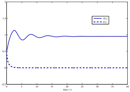
Figure 1 shows the numerical solutions of the SIS model with p = e2, δ = 1.1 (p/δ < e2), a = 2.0, µ = 2.0, γ =
ε = 1.0; hence R0 < 1. In this case ¯I0 = 0 and ¯N0) ' 0.9523. In Figure 1, bothI(· · · dot) andN(−solid) are attracted by the disease-free equilibrium, i.e. ( ¯I,N¯) →
( ¯I0,N¯0) = (0,0.9523).
0 5 10 15 20 25 30 35 40
−0.5 0 0.5 1 1.5 2
time ( t)
[image:7.595.57.285.347.509.2]N(i) I(t)
Figure 1: The numerical solutions of the SIS model with p/δ < e2 andR
0<1, whereτ= 2.0.
0 5 10 15 20 25 30 0
0.5 1 1.5 2
time ( t)
0 10 20 30 40 50 60 70 80 90 100 −0.5
0 0.5 1 1.5 2 2.5 3 3.5 4
time ( t)
Figure 2: The numerical solutions of the SIS model with p/δ > e2 and R
0 <1; where τ = 1.0 (left) and τ = 3.0 (right).
Next, Figure 2 compares the numerical solutions with different delay τ. Here we set p = 15, δ = 1.1 (p/δ > e2), a= 2.0, µ= 2.0, γ = 1.0, ε= 1.0. We can see that
the delay affects the dynamical behaviour of the numeri-cal solutions. We can see that the solution forI(t) is at-tracted by ¯I0= 0, while the solution forN(t) is changed its stability from asymptotic stability (Figure 2(left)) to periodic behaviour (Figure 2(right)).
4.2
Case
R
0>
1
For the case that R0 >1, Figure 3 shows the numerical experiments of the SIS epidemic model with p=e2, δ = 1.1 (p/δ < e2), a = 2.0, µ = 5.0, γ = 1.0, ε = 0 when
τ = 1.0 andτ = 3.0. The results indicate that ifR0>1,
I and N are attracted by the endemic equilibrium, i.e. ( ¯I,N¯)→( ¯I+,N¯+).
0 5 10 15 20 25 30 0
0.5 1 1.5
time ( t)
0 10 20 30 40 50 60 70 80 90 100 0
0.5 1 1.5
time ( t)
Figure 3: The numerical solutions of the SIS model with p/δ < e2 and R
0 >1; where τ = 1.0 (left) and τ = 3.0 (right).
In addition, Figure 4 shows that when p/δ > e2. Here we set p= 15, δ = 1.1 (p/δ > e2), a= 2.0, µ= 5.0, γ = 1.0, ε = 0 The numerical solutions oscillate about the endemic equilibrium. Figure 4(left) and Figure 4(right) represent the solutions when τ = 1.5 and τ = 1.65, re-spectively. We can see that the behaviour of the solutions changes from a solution converging to the equilibrium to a periodic solution. Hence, a Hopf bifurcation occurs when τ is sufficiently large and R0>1.
0 20 40 60 80 100 120 140 160 180 200 0
0.5 1 1.5 2
time ( t)
0 20 40 60 80 100 120 140 160 180 200 0
0.5 1 1.5 2
[image:7.595.309.549.535.613.2]time ( t)
Figure 4: The numerical solutions of the SIS model with p/δ > e2 andR
0 >1; where τ = 1.5 (left) andτ = 1.65 (right).
Note that in Figure 4, we can see that the numerical so-lution undergoes a Hopf bifurcation whenτis sufficiently large. Suppose that τ∗ is the bifurcation point. We can
see that τ∗ ∈ (1.5,1.65). The study of Hopf bifurcation
[image:7.595.53.290.580.658.2]References
[1] K. L. Cooke, P. V. D. Driessche, and X. Zou, “In-teraction of maturation delay and nonlinear birth in population and epidemic models,”Journal of
Math-ematical Biology, vol. 39, no. 4, pp. 332–352, 1999.
[2] J. Wei and X. Zou, “Bifurcation analysis of a pop-ulation model and the resulting SIS epidemic model with delay,” Journal of Computational and Applied
Mathematics, vol. 197, no. 1, pp. 169–187, 2006.
[3] X. Q. Zhao and X. Zou, “Threshold dynamics in a delayed SIS epidemic model,”Journal of
Mathemat-ical Analysis and Applications, vol. 257, no. 2, pp.
282–291, 2001.
[4] W. S. C. Gurney, S. P. Blythe, and R. M. Nisbet, “Nicholson’s blowflies (revisited),”Nature, vol. 287, pp. 17–21, 1980.
[5] Q. X. Feng and J. R. Yan, “Global attractivity and oscillation in a kind of Nicholson’s blowflies,”
Jour-nal of Biomathematics, vol. 17, no. 1, pp. 21–26,
2002.
[6] I. Gy¨ori and S. I. Trofimchuk, “On the existence of rapidly oscillatory solutions in the Nicholson blowflies equation,” Nonlinear Analysis: Theory,
Methods and Applications, vol. 48, no. 7, pp. 1033–
1042, 2002.
[7] E. Kunnawuttipreechachan, “The stability analysis of discrete numerical methods for the delay nichol-son’s blowflies equations and related problems,” Ph.D. Thesis, Brunel University, 2009.
[8] S. H. Saker and S. Agarwal, “Oscillation and global attractivity in a periodic Nicholson’s blowflies model,” Mathematical and Computer Modelling, vol. 35, no. 7-8, pp. 719–731, 2002.
[9] H. L. Smith,Monotone Dynamical Systems: An In-troduction to the Theory of Competitive and
Coopo-rative Systems. USA: American Mathematical
So-ciety, 1995.
[10] V. L. Kocic and G. Ladas,Global Behaviour of Non-linear Difference Equations of Higher Order with
Ap-plications. Netherlands: Kluwer Academic