Introspection for convolutional automatic speech recognition

187

Introspection for convolutional automatic speech recognition

Andreas KrugandSebastian Stober

University of Potsdam, Research Focus Cognitive Sciences Karl-Liebknecht-Str. 24/25, 14476 Potsdam, Germany

{ankrug, sstober}@uni-potsdam.de

Abstract

Artificial Neural Networks (ANNs) have expe-rienced great success in the past few years. The increasing complexity of these models leads to less understanding about their decision processes. Therefore, introspection techniques have been proposed, mostly for images as input data. Patterns or relevant regions in images can be intuitively interpreted by a human observer. This is not the case for more complex data like speech recordings. In this work, we investigate the appli-cation of common introspection techniques from computer vision to an Automatic Speech Recog-nition (ASR) task. To this end, we use a model similar to image classification, which predicts let-ters from spectrograms. We show difficulties in applying image introspection to ASR. To tackle these problems, we propose normalized aver-aging of aligned inputs (NAvAI): a data-driven method to reveal learned patterns for prediction of specific classes. Our method integrates information from many data examples through local introspection techniques for Convolutional Neural Networks (CNNs). We demonstrate that our method provides better interpretability of letter-specific patterns than existing methods.

1 Introduction

Artificial Neural Networks (ANNs) perform incredibly well in many fields of application, even out-performing humans. In particular, deep learning (DL) has been used with great success in a variety of tasks. The most successful applications of DL are in computer vision, like image classification (Krizhevsky et al., 2012) or segmentation (Chen et al., 2014). Moreover, DL performs well in audio processing, like automatic speech recognition (Bahdanau et al.,2016) or machine translation (Wu et al.,2016). One reason for the success of these models is the increase in their complexity by implementing deeper or wider network layers (Szegedy et al.,2015). While this allows the model to learn more complex patterns for solving its

task, it is becoming more difficult to interpret how it accomplishes it (Yosinski et al., 2015). Several introspection techniques were proposed to shed light on the decision processes in ANNs (Zeiler and Fergus 2014,Springenberg et al. 2014,Selvaraju et al. 2016). However, most of them come with restrictions on the network architecture or the type of task that is solved. In particular, most methods focus on interpretability of ANNs in computer vision. The reason for this is that evaluating the results from introspection techniques on images is intuitive for a person. This is not the case for more complex data like audio waveforms or multi-channel data like Electroencephalography (EEG) recordings. Applying introspection techniques from computer vision to this kind of data is possible, but evaluating the results is hard, as a human expert cannot easily interpret the input data in the first place.

In this work, we investigate the application of several introspection techniques to the domain of Automatic Speech Recognition (ASR). To make the task of ASR similar to image classification, we use a fully-convolutional ANN for letter-wise prediction from audio spectrograms. We identify problems in applying introspection techniques from computer vision to the ASR domain. To overcome these difficulties, we propose normalized averaging of aligned inputs (NAvAI): a data-driven introspection method for interpreting speech recognition.

2 Related Work

In computer vision, Convolutional Neural Net-works (CNNs) are the most common choice of network architecture (Szegedy et al.,2015). As we want to adapt techniques from this domain, we focus on introspection methods developed for CNNs.

the original input, for example the deconvolutional network approach by Zeiler and Fergus 2014 or layer-wise relevance propagation (Bach et al., 2015). The second category are global introspection techniques that infer input patterns or characteristics which activate particular neurons, like activation maximization (Erhan et al. 2009,Yosinski et al. 2015).

2.1 Local introspection

Local introspection traces back signals to a particular input source. This means inferring, which parts of an input sample were important for the prediction. The backpropagated signal comes either from pre-softmax activations or the softmax-logits of an ANN classifier’s output layer. The common way is to trace back the result of the output layer as a one-hot vector, so only class-specific information are retained (Springenberg et al.,2014). This means that the position of highest activation is set to 1, while all other positions are set to 0.

A simple and fast way to infer the contribution of in-put values to the classification score is to perform sen-sitivity analysis. This method computes the (squared) partial derivatives of output scores with respect to the values of a particular input sample (Gevrey et al., 2003). Another method is to use deconvolutional net-works, which invert the data flow of a convolutional classifier network to reconstruct the input (Zeiler and Fergus,2014). The backward pass also includes units that revert max-pooling operations. This is done by storing the maximum positions before pooling in so-called switches (Zeiler and Fergus,2014).

Another local introspection method is guided backpropagation (Springenberg et al., 2014). This technique is based on gradient backpropagation but integrates information about the forward pass. For a network which uses Rectified Linear Unit (ReLU) activation, the authors propose to only backpropagate positive gradients, where the corresponding forward activation is positive as well (Springenberg et al., 2014). The authors also report that introspection using the deconvolutional network approach byZeiler and Fergus 2014performs poorly for higher layers, where neurons can be maximally activated by a wider variety of input signals. Their method does not show this drop in performance for higher layers. Guided backpropagation reveals detailed features in the input which are important for the prediction, but is not strongly class-discriminative.

Selvaraju et al. 2016 introduced the class-discriminative Gradient-weighted Class

Activa-tion Mapping (Grad-CAM), which identifies low-resolution regions of importance in the input. Grad-CAM first computes importance weights for each feature map in one layer. This is done by global average pooling gradients of the prediction score with respect to the feature maps. These importance weights are used to compute a weighted sum of forward activa-tions, which represent the influence on the predicted class. The authors use a ReLU on the weighted sums, to only show positive influences on the prediction. By using their method to mask the result of guided backpropagation, which they call guided Grad-CAM, they get both class-specificity and high resolution in relevant input values (Selvaraju et al.,2016).

All of those local introspection methods only reveal information about a single input sample. This could help understanding particular decisions, for example wrong classifications. For revealing decision processes of an ANN as a whole, global introspection is essential.

2.2 Global introspection

The most common global introspection technique is activation maximization (AM) (Erhan et al.,2009). AM is independent of the input and can be used to find patterns which activate particular features. This method optimizes the input, such that the activation of a particular feature is maximized. Such a feature could be a single neuron at any position of the network. For classifiers, the most interesting feature is the output neuron of the predicted class. The op-timization target can be the corresponding activation either before or after applying the softmax. It is also possible to visualize optimal inputs for a whole layer, as in Google DeepDream (Mordvintsev et al.,2015). However, the input optimization approach has some drawbacks. Optimal inputs tend to be unnatural and noisy, thus cannot be interpreted (Nguyen et al.,2015). Therefore, it is crucial to regularize, for example by total variation (Mahendran and Vedaldi,2015) or a Generative Adversarial Network (GAN) objective (Nguyen et al.,2016) to penalize unnatural data. Even with regularized optimization, the optimal input needs to be interpretable. This means a human has to be able to assess, whether patterns in the optimized input are related to a certain class.

2.3 Introspection for audio

a human observer. Whether an introspection technique performs well is mostly measured by how plausible the result is for a person. This is not an objective quan-tification, but it indicates how similar the ANN deci-sions are to the human perception. However, this is not possible for all types of data. For example, when using waveforms as input to an audio-classification task like ASR, it is not intuitive to assess the meaningfulness of important regions or optimal inputs. To our knowl-edge there are no comparable introspection techniques for ANN in speech recognition tasks. However, this is not the first attempt to understand ANNs for speech recognition. Several studies explored representations of speech in ANNs for acoustic modelling, for ex-ample multi-layer perceptrons (Nagamine et al. 2015, Nagamine et al. 2016,Nagamine and Mesgarani 2017) or Deep Belief Networks (Mohamed et al.,2012).

3 Methods

3.1 Automatic Speech Recognition

The use of CNNs for speech is not uncommon. However, they are often used as part of complex hybrid models, for example involving Hidden Markov Models (Abdel-Hamid et al.,2014) or Recurrent Neu-ral Networks (Trigeorgis et al.,2016). Such complex models are much harder to introspect than fully-convolutional ones. CNNs are also used for speech-related tasks different from ASR, like learning spec-trum feature representations (Cummins et al.,2017).

For ASR, we implement a fully-convolutional architecture to apply introspection techniques from computer vision. To this end, we are using an archi-tecture based on Wav2Letter (Collobert et al.,2016). This model is a fully-convolutional neural network, which predicts letters from spectrograms. We train the network on z-normalized spectrograms, scaled to 128 mel-frequency bins. Each letter prediction can use 206 time steps due to the receptive field of the convolutions. We use whole-sequence audio record-ings from the LibriSpeech corpus (Panayotov et al., 2015). Training and architecture are described in detail in (Kunze et al.,2017). Different to Kunze et al. we slightly changed the number of neurons per layer to powers of two (250 to 256 neurons and 2000 to 2048 neurons). Moreover, we used a vocabulary with repetition characters likeCollobert et al. 2016used with their Auto Segmentation Criterion (ASG) loss.

3.2 Activation Maximization

We visualize important features by computing the optimal input for activating a particular neuron. We

used L1- and L2-regularization to avoid unnatural noisy results, both with a scale of 0.001. The optimization was initialized with a206×128input (the receptive field size) using a Xavier uniform initializer (Glorot and Bengio,2010). Training was performed to maximize the activation of a particular neuron, using an Adam optimizer (Kingma and Ba, 2014) with learning rate 0.05 for 250 steps. We applied AM for neurons of different layers to show differences in the complexity of optimal patterns.

3.3 Preparing the data for introspection

Our ASR model predicts all letters for a given speech recording at once, but we are interested in determining the important regions for single predicted letters. Therefore, we perform our analyses on spectrogram frames, which are predicted as only one letter. Based on the receptive field size, we perform introspection on spectrogram frames of width 206. Moreover, we only investigate spectrogram frames predicted as letters ’a’ to ’z’, because blank and repetition charac-ters would not be interpretable for a human observer. For training and evaluation, our neural network uses same-padding with zeros. To avoid biasing our introspection results due to padding, we only analyze spectrogram frames without padding. Because we are training with whole sentences, most of the letters are predicted from spectrogram frames without padding.

3.4 Local introspection

For a spectrogram frame of interest, we first perform a forward pass through the network, while storing all layers’ activations and the output scores. To find important positions in the input data, we perform different methods for propagating back the prediction score. In particular, we are using sensitivity analysis (Gevrey et al., 2003) and layer-wise relevance propagation (LRP) (Montavon et al.,2017). As initial value for the backward pass, we use a vector which is set to 1 for the predicted class and 0 for all other positions. We call this vectorR(out).

We did not investigate guided backpropagation, because we rely on getting class-discriminative introspection results. We also did not use Grad-CAM, because of the 1D-convolutions in our network. As our input data is treated as 128 one-dimensional channels, applying Grad-CAM to our network would only identify important regions over the time dimension. This means, we would not be able to identify which frequencies are important.

input spectrogram frame, as shown in Equation 1. The resulting gradient-based relevancesR(0)can be interpreted as positions in the inputx, which increase or decrease the prediction score upon change.

R_i(0)=∂R

(out)

∂xi

(1)

Different to sensitivity, LRP aims to map high relevances to input positions that have causedR(out)_. We performed non-Taylor-type LRP, which we adapted from Equation 56 inBach et al. 2015:

R(_i←jl,l+1)=zij zj

·R_j(l+1) (2)

where i refers to the neuron in the lower layer l andj to the neuron in the higher layerl+ 1. This original rule means, that relevances are propagated back based on the ratio of local (zij) and global (zj)

pre-activations. The pre-activations are outputs of the convolution for a neuronjeither masking all lower layer neurons but neuroni(local) or not masking any neurons (global). Hence, the ratiozij

zj is the relative influence of a neuronion the pre-activation of neuron j. This allows to distribute the relevance from neuron j to the lower layer neurons while conserving the sum of relevance values (compare Equation5).

Computing these ratios is computationally ex-pensive for more complex neural networks, as it is necessary to compute the contribution of every value iof the lower layer to every valuej of the higher layer through the convolutions. For example, in the input layer of our network, it is necessary to compute local pre-activations from 128×206 input values to256×80output values. This corresponds to 500 million local pre-activations in the first layer.

Applying Equation 2 is not straightforward in our speech recognizer network. This is due to two major differences to the image classification networks that Bach et al. 2015 used. Firstly, our network involves negative input values from z-normalized mel-spectrograms. Secondly, after each convolution, batch normalization is applied before the ReLU activation. This allows convolution outputs to change their sign before entering the ReLU activation. In order to account for negative values and the effects of batch normalization, we adapt Equation2as follows. We compute the ratio between local and global pre-activations using the absolute value of the global activation. This preserves the sign of local pre-activations for comparison to the convolution output after applying batch normalization. The magnitude

of the neuron influence is not changed. For avoiding division by zero, we add a small value= 1e-21to the absolute value of global pre-activation. This ratio is multiplied with the sign of the output value after applying batch normalization (bn), shown in Equation 3. With this approach, a positive ratio indicates that a local pre-activation supports the output after batch normalization, because they have the same sign. We backpropagate the relevance as shown in Equation4.

rij=

zij |zj|+

·sgn(bn(zj)) (3)

R(_i←jl,l+1)=rij·R_j(l+1) (4)

The original rule in Equation 2is satisfying the conservation law

X

i

R(_i←jl,l+1)=R_j(l+1) (5)

where no relevance may be lost by distributing the value to lower layer neurons. In our adaptation, this conservation law is not satisfied, because we change the sign of some ratios to correct for batch normal-ization. As this procedure does not change absolute values, we do not lose any information about the evances. Furthermore, using the original rule, rel-evances can become unbounded for negative ratios

zij

zj. To avoid absolute relevances to become very large, we scale the values by the maximum absolute relevance value in each step of LRP. Scaling the relevances is also violating the conservation law in Equation5. However, the relevances still contain the same information, as the ratio between all relevances is conserved.

3.5 Normalized averaging of aligned inputs

would get averaged out. Therefore, before comput-ing average frames, NAvAI aligns the spectrogram frames as described below. Computing the average over (aligned) letter-specific spectrogram frames re-tains information about what is common to all frames. However, this is not necessarily exclusive to spectro-gram frames of this particular letter. There might be in-formation, which is contained for all predicted letters. Therefore, our method normalizes the letter-averaged spectrogram frames by subtracting the mean over spec-trogram frames predicted as any letter ’a’ to ’z’.

3.6 Alignment of spectrogram frames

For proper alignment between predicted letter and spectrogram, we facilitate the introspection techniques from Section3.4. We follow the hypothesis, that the time step, where a predicted letter actually occurs, is the one that is most important for the prediction score. We infer this position from local introspection results using sensitivity analysis and LRP. Positive rele-vances from LRP identify values, which have caused the prediction score. Therefore, we use the maximum position from LRP. In contrast, sensitivity can be meaningful both at the maximum and minimum value position. Positive values imply importance of positions, because increasing them would make the prediction more certain. Negative gradients are of interest as well, because they show where a change in input value causes the prediction certainty to drop. Most of the predictions are already very close to being a one-hot vector as softmax-output. Then, there might be no or only a small gradient for increasing the prediction certainty. In this case, the minimum value position from sensitivity might be more appropriate than the maximum value position. The alignment procedure crops the spectrogram frames on one side, such that the determined positions are in the center.

4 Results & Discussion

4.1 Optimal inputs by activation maximization

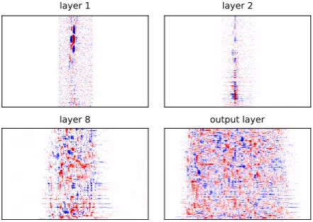
We performed AM for neurons of different layers. For visualization, we chose neurons which are maximally activated for the prediction of letter ’a’ in a randomly chosen spectrogram frame. In the output layer, this neuron corresponds to the predicted letter (here it is the ’a’-neuron). As the outputs of the three topmost layers are one-dimensional, we use the neuron of highest activation. In all other layers, we chose neurons with highest average activation over the time dimension. We only show optimization of strongly activated neurons, because they are evidently sensitive

to some pattern and potentially letter-specific. In Figure 1, we representatively show four different layers of the network. The top row shows optimal inputs for a neuron in the first and second layer. In those layers, AM reveals patterns, which can be in-terpreted as features in the spectrogram. For example, the input layer neuron detects a shift of intensity towards higher frequencies. The second-layer neuron combines low-level features, so it is sensitive to different changes in frequency intensities, particularly of lower frequencies. In contrast, optimizing neuron

layer 1 layer 2

layer 8 output layer

Figure 1: Optimal inputs for neurons in different layers of the network. Each shown neuron has highest activation for predicting letter ’a’ in the respective layer. Optimal inputs to bottom layers (top row) are still interpretable as features in the spectrogram. The higher layers (bottom row), in particular the output neuron for ’a’ (bottom right), do not look like spectrograms and cannot be interpreted as particular features which the neuron is sensitive to. The axes are equal to the spectrogram frames in Figure2.

output in higher layers (bottom row) does not reveal any interpretable patterns. Those neurons are sensitive to a large variety of different patterns, so that a single optimal input is not natural anymore. This is a common problem for AM. Still, it is easier to detect unnatural but related patterns in real-world images than in audio spectrograms.

To obtain more natural results, one possibility would be using stronger regularization techniques like a GAN penalty. On the other hand, using stronger regularization interferes with determining the actual learned patterns. Regularizing is therefore favoring results similar to data over actual insight in the model. For our speech recognizer, we can conclude that the model did not learn a single abstract representation for the letters. This is not surprising, as the same letter is not pronounced equally in every context.

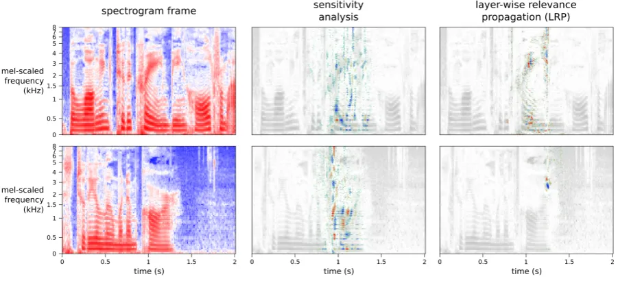
zero-Figure 2: Local introspection using sensitivity analysis and LRP.Left: Two spectrogram frames, both predicted as letter ’a’. By propagating the prediction score back through the network, important regions are identified.Center: Sensitivity analysis results.Right: Relevances using LRP. The results of both methods are visualized as an overlay on top of the original spectrogram. Blue values indicate negative sensitivity/relevance, red indicates positive values.

areas in the beginning and end of the optimal input. This implies that the network capacity is not fully uti-lized for the prediction and could still be compressed.

4.2 Sensitivity analysis and LRP

We performed sensitivity analysis and LRP for all spectrogram frames. Here, we show characteristics of these methods based on two spectrogram frames predicted as letter ’a’. Figure 2 shows those two spectrogram frames (left) and the local introspection results. The sensitivity values (center) and LRP-based relevances (right) are visualized superimposed on the input spectrogram. Both methods differ strongly in what they identify as important for the prediction.

Sensitivity analysis identifies relevant positions in a larger area and includes more data points than LRP. As we assumed, if the prediction already was certain, sensitivity analysis is resulting in mostly negative values, as in the top example. In the bottom example, there are more positive gradients, indicating a less certain prediction. Moreover, sensitivity analysis identifies important regions close to center of the spectrogram frame.

The relevances backpropagated with LRP are much more position-specific than sensitivity values. The top example shows fewer relevant positions. In the bottom example, relevance is assigned to only two small regions. This indicates that LRP identifies important positions, but emphasizes the most relevant ones. We assume, this is due to having negative

input values. As mentioned above, relevances can become unbounded for negative input values, which we prevented by scaling them. However, this does not reduce possible large differences between weak and strong relevances. We also observe that LRP identifies regions as relevant, which are further away from the center of the spectrogram frame.

Neither sensitivity analysis nor LRP reveal patterns, which can be interpreted as typical letters for the network. Furthermore, different spectrogram frames predicted as the same letter do rarely show common patterns. We would expect that in most cases impor-tant regions for predicting letter ’a’ are formants in the spectrogram, which are characteristic for vowels. The second example in Figure2is one of many examples, where this expectation is not met. Sensitivity analysis shows that the beginning of the utterance is important, because highly sensitive positions are distributed over all frequencies in one time point. This can be ex-plained for the model, since it could have learned the context around the formant pattern. The LRP result is identifying two small regions in the spectrogram both of negative values in the spectrogram. Although this might be valid for what is important for the model, this cannot be interpreted as features of an ’a’.

4.3 Global introspection

'a'

't'

all

letter

alignment

minimum sensitivity maximum

sensitivity

maximum LRP not

aligned

'a'

't'

mean

spectr

ogr

am

letter-speci

fi

c

patt

erns

norm

ali

zer

-=

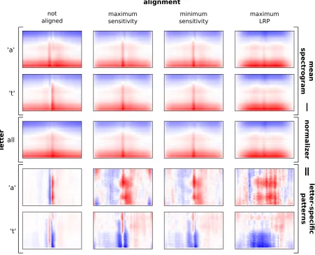
Figure 3: Averaging and normalizing letter-specific spectrogram frames.Top two rows: Mean inputs over spectrograms predicted as letter ’a’ and ’t’, respectively.Middle row: Average spectrogram frame over all letters, which is used for normalization.Bottom two rows: By subtracting the mean over all letters from the letter-averaged spectrograms, we obtain patterns specific to the prediction of certain letters. Each analysis was performed with different alignment methods, of which each is visualized in a column. Thesecond to fourth columncorrespond to aligning the spectrograms frames to the predicted letter based on local introspection. As comparison, thefirst columnpresents the averaging results for the unaligned spectrogram frames. The axes are equal to the spectrograms in Figure2. Values in each frame are normalized, such that the absolute maximum is 1.

and normalize them. The alignment procedure crops the frames, so they are centered to the most important position. Because of this, the beginning and end of the averaged frame implicitly has lower values.

Mean spectrogram frames over letters Figure3 exemplifies the mean spectrogram frames for letters ’a’ and ’t’ (top two rows). It is not possible to see interpretable differences between particular letters. Therefore, we cannot tell anything about the quality of the alignment methods as well. Interestingly, for all letters there are higher mean values in the center of unaligned mean spectrogram frames where only the position is slightly shifted comparing the letters. This

mean is very similar to the letter-specific means. This shows that there is information common to all letters, which overshadows the spectrogram features that are relevant for prediction. More precisely, this information is not only common to the letters, but to spectrograms in general. For example, in speech, there is higher intensity of low frequencies than of high frequencies. This is reflected in the mean spectrograms, where the mean value decreases with higher frequency.

Mean spectrogram frame normalization To re-veal where the differences between the letter-specific patterns are, we normalized each letter-averaged spectrogram frame with the mean over all letters. Figure3visualizes this procedure, where the mean over all letters (middle row) is subtracted from the exemplary mean frames over letters ’a’ and ’t’ (top two rows). The resulting average spectrogram frames after normalization are shown in the bottom two rows of Figure3. With normalization, we obtain the final result of our NAvAI method and we are able to observe letter-specific patterns.

Patterns in normalized mean spectrogram frames We emphasize that the normalized frames (bottom two rows of Figure3) are not spectrograms anymore. Positive (red) and negative (blue) values indicate, where the average over one letter is higher or lower than the mean over all letters, respectively. This can lead to positive values where the (average) spectrogram was negative, and vice versa. Moreover, our method is not identifying which particular features are used by the network for prediction. For example, if NAvAI reveals two formants for a particular letter, it is not certain that both are used for the prediction.

First of all, we averaged spectrogram frames without alignment (first column in Figure3). There are no letter-specific patterns visible in the resulting frames. For all letters, the normalized frame only shows a transition from positive to negative values (or the other way round) in the center. This simply reflects the above mentioned high intensities in the center, which are slightly shifted for different letters.

With all investigated alignment methods, we can observe a clear difference between the patterns for different letters. For predicting letter ’a’, the network is detecting a stronger signal at the center and right of it for sensitivity-based and LRP alignments. Also for all alignments, two formants are clearly visible at around 700 Hz and 2700 Hz. This pattern makes sense, as vowels are combinations of different

formants. While all alignment methods show this pattern, it is more wide-spread across time using LRP.

Similarly, we can observe a letter-specific pattern for the letter ’t’. For sensitivity-based alignments, there is a quick change from lower to higher signal and back in the center. This transition occurs in all frequencies, while it is more pronounced in the higher ones. This corresponds to the typical pattern of plosives. Their release burst is characterized by a high intensity of all frequencies in a very short time span. With LRP-based alignment, we did not observe this pattern. From the observations for letter ’a’, we know that the signal is more wide-spread for LRP. This is not affecting the observed formant pattern of letter ’a’, but it affects the plosive pattern. Here, the signal of interest spans the frequency dimension. Spreading the strong signal wider in the time dimension causes averaging out the interesting pattern. The weaker signal of low frequencies is detected with both sensitivity and LRP, because this is more consistent in the time dimension. The wide spread of signals when aligning by maximum LRP indicates that the letters were not properly aligned to the spectrogram.

The alignment by minimum or maximum sen-sitivity both revealed letter-specific patterns which also are specific in the time dimension. There is only slight difference between minimum and maximum sensitivity alignment, but the resulting normalized mean spectrogram frames seem to be more specific when aligning at the minimum sensitivity. We cannot guarantee that the alignment centers the spectrograms at the real occurrence of the letter. This can be seen in the typical patterns for ’a’, which are right of the center. However, as long as the alignment is consistent, we still get meaningful results. We suspected that the network learns to facilitate release bursts of plosives in the center of prediction frames. If this was true, alignment should not change the center position much for letters that are mostly pronounced as plosives. This idea is supported by the shown results, as there is a much smaller difference between aligned and unaligned mean spectrogram frames for ’t’ compared to ’a’. Patterns of all letters are provided

in Supplemental MaterialA.

5 Conclusion

local introspection with sensitivity analysis and LRP does not give much insight into the network. Global introspection with weakly regularized AM was only producing interpretable patterns for lower layers.

We introduced NAvAI as a novel introspection method, which determines class-specific features by averaging over examples for each class. This approach adapts simple averaging to specific properties of the ASR task, by aligning letters to spectrograms through local introspection techniques and normalization. We showed that our method is capable of revealing in-terpretable patterns, which are common to predicting particular letters. Although demonstrated for ASR, NAvAI is generally applicable to other domains.

This work did not cover, whether there are different patterns corresponding to particular contexts or pronunciation of letters. In future work, the classes will be separated into different pronunciations, for example by facilitating information about phonemes. Although the patterns are interpretable, some knowledge about features in spectrograms is needed. Evaluating the introspection as a sound example would be far more intuitive. Therefore, future work will cover synthesizing sound samples from the intro-spection results or working with waveforms directly. This work pinpointed several issues, where common introspection techniques fail for CNN-based ASR. Following our results, we will further develop or adapt introspection techniques and optimize the architecture towards better applicability of introspection.

Acknowledgments

This research has been funded by the Federal Ministry of Education and Research of Germany (BMBF) and supported by the donation of a GeForce GTX Titan X graphics card from the NVIDIA Corporation.

References

Ossama Abdel-Hamid, Abdel-rahman Mohamed, Hui Jiang, Li Deng, Gerald Penn, and Dong Yu. 2014. Convolutional neural networks for speech recognition.

IEEE/ACM Transactions on audio, speech, and language processing, 22(10):1533–1545.

Sebastian Bach, Alexander Binder, Gr´egoire Montavon, Frederick Klauschen, Klaus-Robert M¨uller, and Wo-jciech Samek. 2015. On pixel-wise explanations for non-linear classifier decisions by layer-wise relevance propagation. PloS one, 10(7):e0130140.

Dzmitry Bahdanau, Jan Chorowski, Dmitriy Serdyuk, Philemon Brakel, and Yoshua Bengio. 2016. End-to-end attention-based large vocabulary speech

recognition. InAcoustics, Speech and Signal Process-ing (ICASSP), 2016 IEEE International Conference on, pages 4945–4949. IEEE.

Liang-Chieh Chen, George Papandreou, Iasonas Kokki-nos, Kevin Murphy, and Alan L Yuille. 2014. Semantic image segmentation with deep convolutional nets and fully connected crfs. arXiv preprint arXiv:1412.7062.

Ronan Collobert, Christian Puhrsch, and Gabriel Syn-naeve. 2016. Wav2letter: an end-to-end convnet-based speech recognition system. CoRR, abs/1609.03193.

Nicholas Cummins, Shahin Amiriparian, Gerhard Hagerer, Anton Batliner, Stefan Steidl, and Bj¨orn W Schuller. 2017. An image-based deep spectrum feature representation for the recognition of emotional speech. In Proceedings of the 2017 ACM on Multimedia Conference, pages 478–484. ACM.

Dumitru Erhan, Yoshua Bengio, Aaron Courville, and Pascal Vincent. 2009. Visualizing higher-layer features of a deep network. University of Montreal, 1341(3):1.

Muriel Gevrey, Ioannis Dimopoulos, and Sovan Lek. 2003. Review and comparison of methods to study the contribution of variables in artificial neural network models. Ecological modelling, 160(3):249–264.

Xavier Glorot and Yoshua Bengio. 2010. Understanding the difficulty of training deep feedforward neural net-works. InProceedings of the thirteenth international conference on artificial intelligence and statistics, pages 249–256.

Diederik P Kingma and Jimmy Ba. 2014. Adam: A method for stochastic optimization. arXiv preprint arXiv:1412.6980.

Alex Krizhevsky, Ilya Sutskever, and Geoffrey E Hinton. 2012. Imagenet classification with deep convolutional neural networks. In F. Pereira, C. J. C. Burges, L. Bottou, and K. Q. Weinberger, editors, Advances in Neural Information Processing Systems 25, pages 1097–1105. Curran Associates, Inc.

Julius Kunze, Louis Kirsch, Ilia Kurenkov, Andreas Krug, Jens Johannsmeier, and Sebastian Stober. 2017. Transfer learning for speech recognition on a budget. InProceedings of the 2nd Workshop on Representation Learning for NLP, pages 168–177. Association for Computational Linguistics.

Aravindh Mahendran and Andrea Vedaldi. 2015. Under-standing deep image representations by inverting them. In Proceedings of the IEEE conference on computer vision and pattern recognition, pages 5188–5196.

Gr´egoire Montavon, Sebastian Lapuschkin, Alexander Binder, Wojciech Samek, and Klaus-Robert M¨uller. 2017. Explaining nonlinear classification decisions with deep taylor decomposition. Pattern Recognition, 65:211–222.

Alexander Mordvintsev, Christopher Olah, and Mike Tyka. 2015. Inceptionism: Going deeper into neural networks. Google Research Blog. Retrieved June, 20(14):5.

Tasha Nagamine and Nima Mesgarani. 2017. Understand-ing the representation and computation of multilayer perceptrons: A case study in speech recognition. In

International Conference on Machine Learning, pages 2564–2573.

Tasha Nagamine, Michael L Seltzer, and Nima Mesgarani. 2015. Exploring how deep neural networks form phonemic categories. In Sixteenth Annual Confer-ence of the International Speech Communication Association.

Tasha Nagamine, Michael L Seltzer, and Nima Mesgarani. 2016. On the role of nonlinear transformations in deep neural network acoustic models. InInterspeech, pages 803–807.

Anh Nguyen, Alexey Dosovitskiy, Jason Yosinski, Thomas Brox, and Jeff Clune. 2016. Synthesizing the preferred inputs for neurons in neural networks via deep generator networks. InAdvances in Neural Information Processing Systems, pages 3387–3395.

Anh Nguyen, Jason Yosinski, and Jeff Clune. 2015. Deep neural networks are easily fooled: High confidence predictions for unrecognizable images. InProceedings of the IEEE Conference on Computer Vision and Pattern Recognition, pages 427–436.

Vassil Panayotov, Guoguo Chen, Daniel Povey, and Sanjeev Khudanpur. 2015. Librispeech: an asr corpus based on public domain audio books. In Acoustics, Speech and Signal Processing (ICASSP), 2015 IEEE International Conference on, pages 5206–5210. IEEE.

Ramprasaath R. Selvaraju, Abhishek Das, Ramakrishna Vedantam, Michael Cogswell, Devi Parikh, and Dhruv Batra. 2016. Grad-cam: Visual explanations from deep networks via gradient-based localization. CoRR, abs/1610.02391.

Jost Tobias Springenberg, Alexey Dosovitskiy, Thomas Brox, and Martin Riedmiller. 2014. Striving for simplicity: The all convolutional net. arXiv preprint arXiv:1412.6806.

Christian Szegedy, Wei Liu, Yangqing Jia, Pierre Ser-manet, Scott Reed, Dragomir Anguelov, Dumitru Erhan, Vincent Vanhoucke, and Andrew Rabinovich. 2015. Going deeper with convolutions. InProceedings of the IEEE conference on computer vision and pattern recognition, pages 1–9.

George Trigeorgis, Fabien Ringeval, Raymond Brueckner, Erik Marchi, Mihalis A Nicolaou, Bj¨orn Schuller, and Stefanos Zafeiriou. 2016. Adieu features? end-to-end speech emotion recognition using a deep convolu-tional recurrent network. In Acoustics, Speech and Signal Processing (ICASSP), 2016 IEEE International Conference on, pages 5200–5204. IEEE.

Yonghui Wu, Mike Schuster, Zhifeng Chen, Quoc V Le, Mohammad Norouzi, Wolfgang Macherey, Maxim Krikun, Yuan Cao, Qin Gao, Klaus Macherey, et al. 2016. Google’s neural machine translation system: Bridging the gap between human and machine translation. arXiv preprint arXiv:1609.08144.

Jason Yosinski, Jeff Clune, Anh Nguyen, Thomas Fuchs, and Hod Lipson. 2015. Understanding neural networks through deep visualization. arXiv preprint arXiv:1506.06579.

A Supplemental Material

A.1 NAvAI results for letters ’a’ to ’i’

alignment

minimum sensitivity maximum

sensitivity

maximum LRP not

aligned

'a'

'b'

'c'

'd'

'e'

'f'

'g'

'h'

A.2 NAvAI results for letters ’j’ to ’r’

'j'

'k'

'l'

'm'

'n'

'o'

'p'

'q'

'r'

alignment

minimum sensitivity maximum

sensitivity maximumLRP

A.3 NAvAI results for letters ’s’ to ’z’

's'

't'

'u'

'v'

'w'

'x'

'y'

'z'

alignment

minimum sensitivity maximum

sensitivity maximumLRP