Learning Generic Sentence Representations Using
Convolutional Neural Networks
Zhe Gan†, Yunchen Pu†, Ricardo Henao†, Chunyuan Li†, Xiaodong He‡, Lawrence Carin† †Duke University,‡Microsoft Research, Redmond, WA 98052, USA
{zg27, yp42, r.henao, cl319, lcarin}@duke.edu [email protected]
Abstract
We propose a new encoder-decoder ap-proach to learn distributed sentence rep-resentations that are applicable to multiple purposes. The model is learned by using a convolutional neural network as an encoder to map an input sentence into a continuous vector, and using a long short-term mem-ory recurrent neural network as a decoder. Several tasks are considered, including sen-tence reconstruction and future sensen-tence prediction. Further, a hierarchical encoder-decoder model is proposed to encode a sen-tence to predict multiple future sensen-tences. By training our models on a large collection of novels, we obtain a highly generic con-volutional sentence encoder that performs well in practice. Experimental results on several benchmark datasets, and across a broad range of applications, demonstrate the superiority of the proposed model over competing methods.
1 Introduction
Learning sentence representations is central to many natural language modeling applications. The aim of a model for this task is to learn fixed-length feature vectors that encode the seman-tic and syntacseman-tic properties of sentences. Deep learning techniques have shown promising per-formance on sentence modeling, via feedfor-ward neural networks (Huang et al., 2013), re-current neural networks (RNNs) (Hochreiter and
Schmidhuber, 1997), convolutional neural
net-works (CNNs) (Kalchbrenner et al., 2014; Kim,
2014;Shen et al.,2014), and recursive neural net-works (Socher et al.,2013). Most of these models aretask-dependent: they are trained specifically for a certain task. However, these methods may
be-come inefficient when we need to repeatedly learn sentence representations for a large number of dif-ferent tasks, because they may require retraining a new model for each individual task. In this paper, in contrast, we are primarily interested in learning
genericsentence representations that can be used across domains.
Several approaches have been proposed for learn-ing generic sentence embeddlearn-ings. The paragraph-vector model ofLe and Mikolov(2014) incorpo-rates a global context vector into the log-linear neu-ral language model (Mikolov et al.,2013) to learn the sentence representation; however, at predic-tion time, one needs to perform gradient descent to compute a new vector. The sequence autoencoder
ofDai and Le(2015) describes an encoder-decoder
model to reconstruct the input sentence, while the skip-thought model ofKiros et al.(2015) extends the encoder-decoder model to reconstruct the sur-rounding sentences of an input sentence. Both the encoder and decoder of the methods above are mod-eled as RNNs.
CNNs have recently achieved excellent results in various task-dependent natural language applica-tions as the sentence encoder (Kalchbrenner et al.,
2014;Kim,2014;Hu et al.,2014). This motivates us to propose a CNN encoder for learning generic sentence representations within the framework of encoder-decoder models proposed by Sutskever et al. (2014); Cho et al. (2014). Specifically, a CNN encoder performs convolution and pooling operations on an input sentence, then uses a fully-connected layer to produce a fixed-length encoding of the sentence. This encoding vector is then fed into a long short-term memory (LSTM) recurrent network to produce a target sentence. Depending on the task, we propose three models: (i) CNN-LSTM autoencoder: this model seeks to reconstruct the original input sentence, by capturing the in-tra-sentence information; (ii)CNN-LSTM future
you$$$$$$will$$$$$$love$$$$$$it$$$$$$$$$$! you$$will$$$love$$$it$$$$$$$$! i promise$$.
sentence&encoder
sentence&decoder
paragraph& generator
this$$$$$$$is$$$$$$$great$$$$$$$. you$$$$$$will$$$$$$love$$$$$$it$$$$$$$$$$!
!$$$$$$$it$$$$$love$$will$$$you i promise$$.
sentence&encoder sentence&decoder
(a) (b)
[image:2.595.81.521.63.253.2](c)
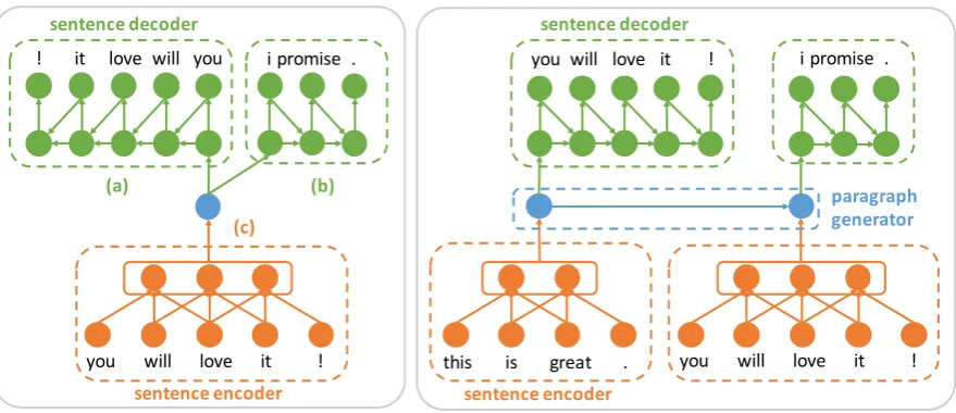
Figure 1: Illustration of the CNN-LSTM encoder-decoder models. The sentence encoder is a CNN, the sentence decoder is an LSTM, and the paragraph generator is another LSTM. (Left) (a)+(c) represents the autoencoder; (b)+(c) represents the future predictor; (a)+(b)+(c) represents the composite model. (Right) hierarchical model. In this example, the input contiguous sentences are:this is great. you will love it! i promise.
predictor: this model aims to predict a future sen-tence, by leveraging inter-sentence information; (iii) CNN-LSTM composite model: in this case, there are two LSTMs, decoding the representation to the input sentence itself and a future sentence. This composite model aims to learn a sentence en-coder that captures bothintra-andinter-sentence information.
The proposed CNN-LSTM future predictor model only considers the immediately subsequent sentence as context. In order to capture longer-term dependencies between sentences, we further introduce a hierarchical encoder-decoder model. This model abstracts the RNN language model ofMikolov et al.(2010) to the sentence level. That is, instead of using the current word in a sentence to predict future words (sentence continuation), we encode a sentence to predict multiple future sen-tences (paragraph continuation). This model is termedhierarchical CNN-LSTM model.
As in Kiros et al. (2015), we first train our proposed models on a large collection of novels. We then evaluate the CNN sentence encoder as a generic feature extractor for 8 tasks: semantic relatedness, paraphrase detection, image-sentence ranking and 5 standard classification benchmarks. In these experiments, we train a linear classifier on top of the extracted sentence features, without additional fine-tuning of the CNN. We show that our trained sentence encoder yields generic
repre-sentations that perform as well as, or better, than those ofKiros et al.(2015);Hill et al.(2016), in all the tasks considered.
Summarizing, the main contribution of this pa-per is a new class of CNN-LSTM encoder-decoder models that is able to leverage the vast quan-tity of unlabeled text for learning generic sen-tence representations. Inspired by the skip-thought model (Kiros et al.,2015), we have further explored different variants: (i) CNN is used as the sentence encoder rather than RNN; (ii) larger context win-dows are considered: we propose the hierarchical CNN-LSTM model to encode a sentence for pre-dicting multiple future sentences.
2 Model description
2.1 CNN-LSTM model
Consider the sentence pair(sx, sy). The encoder,
a CNN, encodes the first sentencesx into a
fea-ture vector z, which is then fed into an LSTM decoder that predicts the second sentencesy. Let
wt
x ∈ {1, . . . , V}represent thet-th word in
sen-tencessx, wherewtxindexes one element in aV
-dimensional set (vocabulary);wt
y is defined
simi-larly w.r.t. sy. Each wordwxt is embedded into
a k-dimensional vector xt = We[wxt], where
We ∈Rk×V is a word embedding matrix (learned),
and notationWe[v]denotes thev-th column of
CNN encoder The CNN architecture in Kim
(2014);Collobert et al.(2011) is used for sentence encoding, which consists of a convolution layer and a max-pooling operation over the entire sen-tence for each feature map. A sensen-tence of lengthT
(padded where necessary) is represented as a matrix X∈Rk×T, by concatenating its word embeddings
as columns,i.e., thet-th column ofXisxt.
A convolution operation involves a filterWc∈
Rk×h, applied to a window ofhwords to produce
a new feature. According toCollobert et al.(2011), we can induce one feature mapc =f(X∗Wc+
b)∈RT−h+1, wheref(·)is a nonlinear activation function such as the hyperbolic tangent used in our experiments,b ∈RT−h+1 is a bias vector, and∗ denotes the convolutional operator. Convolving the same filter with theh-gram at every position in the sentence allows the features to be extracted independently of their position in the sentence. We then apply a max-over-time pooling operation ( Col-lobert et al.,2011) to the feature map and take its maximum value,i.e.,ˆc= max{c}, as the feature corresponding to this particular filter. This pooling scheme tries to capture the most important feature,
i.e., the one with the highest value, for each fea-ture map, effectively filtering out less informative compositions of words. Further, pooling also guar-antees that the extracted features are independent of the length of the input sentence.
The above process describes how one feature is extracted from one filter. In practice, the model uses multiple filters with varying window sizes (Kim,2014). Each filter can be considered as a linguistic feature detector that learns to rec-ognize a specific class ofn-grams (orh-grams, in the above notation). However, since theh-grams are computed in the embedding space, the model naturally handles similarh-grams composed of syn-onyms. Assume we havemwindow sizes, and for each window size, we usedfilters; then we obtain amd-dimensional vector to represent a sentence.
Compared with the LSTM encoders used inKiros et al.(2015);Dai and Le(2015);Hill et al.
(2016), a CNN encoder may have the following ad-vantages. First, the sparse connectivity of a CNN, which indicates fewer parameters are required, typ-ically improves its statistical efficiency as well as reduces memory requirements (Goodfellow et al.,
2016). For example, excluding the number of pa-rameters used in the word embeddings, our trained CNN sentence encoder has 3 million parameters,
while the skip-thought vector ofKiros et al.(2015) contains 40 million parameters. Second, a CNN is easy to implement in parallel over the whole sentence, while an LSTM needs sequential compu-tation.
LSTM decoder The CNN encoder maps sen-tence sx into a vector z. The probability of a
length-T sentence sy given the encoded feature
vectorzis defined as
p(sy|z) = T
Y
t=1
p(wt
y|w0y, . . . , wty−1,z) (1)
where w0
y is defined as a special
start-of-the-sentence token. All the words in the start-of-the-sentence are sequentially generated using the RNN, until the end-of-the-sentence symbol is generated. Specif-ically, each conditional p(wt
y|w<ty ,z), where <
t={0, . . . , t−1}, is specified as softmax(Vht),
whereht, the hidden units, are recursively updated
throughht=H(yt−1,ht−1,z), andh0is defined as a zero vector (h0is not updated during training). Vis a weight matrix used for computing a distribu-tion over words. Bias terms are omitted for simplic-ity throughout the paper. The transition function H(·)is implemented with an LSTM (Hochreiter
and Schmidhuber,1997).
Given the sentence pair (sx, sy), the objective
function is the sum of the log-probabilities of the target sentence conditioned on the encoder repre-sentation in (1):PTt=1logp(wt
y|w<ty ,z). The total
objective is the above objective summed over all the sentence pairs.
Applications Inspired bySrivastava et al.(2015), we propose three models: (i) an autoencoder, (ii) a future predictor, and (iii) the composite model. These models share the same CNN-LSTM model architecture, but are different in terms of the choices of the target sentence. An illustration of the proposed encoder-decoder models is shown in Figure1(left).
which has been shown to be useful to learn the se-mantics of a sentence (Kiros et al.,2015). These two tasks can be combined to create a composite model (iii), where the CNN encoder is asked to learn a feature vector that is useful to simultane-ously reconstruct the input sentence and predict a future sentence. This composite model encour-ages the sentence encoder to incorporate contextual information both within and beyond the sentence. 2.2 Hierarchical CNN-LSTM model
The future predictor described in Section2.1only considers the immediately subsequent sentence as context. By utilizing a larger surrounding context, it is likely that we can learn even higher-quality sentence representations. Inspired by the standard RNN-based language model (Mikolov et al.,2010) that uses the current word to predict future words, we propose a hierarchical encoder-decoder model that encodes the current sentence to predict mul-tiple future sentences. An illustration of the hier-archical model is shown in Figure1(right), with details provided in Figure2.
Our proposed hierarchical model characterizes the hierarchyword-sentence-paragraph. A para-graph is modeled as a sequence of sentences, and each sentence is modeled as a sequence of words. Specifically, assume we are given a paragraph
D = (s1, . . . , sL), that consists of L sentences.
The probability for paragraphDis then defined as
p(D) =YL
`=1
p(s`|s<`) (2)
where s0 is defined as a special start-of-the-paragraph token. As shown in Figure2(left), each
p(s`|s<`)in (2) is calculated as
p(s`|s<`) =p(s`|h(`p)) (3)
h`(p)=LSTMp(h`(p−1) ,z`−1) (4)
z`−1 =CNN(s`−1) (5)
where h(`p) denotes the `-th hidden state of the LSTM paragraph generator, and h(0p) is fixed as a zero vector. The CNN in (5) is as described in Section2.1, encoding the sentences`−1into a vector representationz`−1.
Equation (4) serves as the paragraph-level lan-guage model (Mikolov et al.,2010), which encodes all the previous sentence representationsz<`into a
vector representationh(`p). This hidden stateh(`p)
LSTMS LSTMS
CNN CNN w2v w2v
[image:4.595.306.522.61.186.2](Left) LSTMP (Right) LSTMS
Figure 2: Detailed illustration of the hierarchical CNN-LSTM model. (Left) LSTM paragraph gen-erator. (Right) LSTM sentence decoder.
is used to guide the generation of the`-th sentence through the decoder (3), which is defined as
p(s`|h(`p)) =
T`
Y
t=1
p(w`,t|w`,<t,h(`p)) (6)
where w`,0 is defined as a special start-of-the-sentence token.T`is the length of sentence`, and
w`,tdenotes thet-th word in sentence`. As shown
in Figure2(right), eachp(w`,t|w`,<t,h(`p))in (6) is
calculated as
p(w`,t|w`,<t,h`(p)) =softmax(Vh(`,ts)) (7)
h(`,ts)=LSTMs(h`,t(s)−1,x`,t−1,h(`p)) (8)
where h(`,ts) denotes the t-th hidden state of the LSTM decoder for sentence`,x`,t−1 denotes the word embedding for w`,t−1, andh(`,s0) is fixed as a zero vector for all` = 1, . . . , L. Vis a weight matrix used for computing distribution over words.
3 Related work
Various methods have been proposed for sentence modeling, which generally fall into two categories. The first consists of models trained specifically for a certain task, typically combined with downstream applications. Several models have been proposed along this line, ranging from simple additional com-position of the word vectors (Mitchell and Lapata,
2010;Yu and Dredze,2015;Iyyer et al.,2015) to those based on complex nonlinear functions like re-cursive neural networks (Socher et al.,2011,2013), convolutional neural networks (Kalchbrenner et al.,
2014;Hu et al.,2014;Johnson and Zhang,2015;
The other category consists of methods aiming to learn generic sentence representations that can be used across domains. This includes the para-graph vector (Le and Mikolov,2014), skip-thought vector (Kiros et al.,2015), and the sequential de-noising autoencoders (Hill et al.,2016). Hill et al.
(2016) also proposed a sentence-level log-linear bag-of-words (BoW) model, where a BoW repre-sentation of an input sentence is used to predict ad-jacent sentences that are also represented as BoW. Most recently, Wieting et al.(2016); Arora et al.
(2017);Pagliardini et al.(2017) proposed methods in which sentences are represented as a weighted average of fixed (pre-trained) word vectors. Our model falls into this category, and is most related toKiros et al.(2015).
However, there are two key aspects that make our model different fromKiros et al.(2015). First, we use CNN as the sentence encoder. The combination of CNN and LSTM has been considered in image captioning (Karpathy and Fei-Fei,2015), and in some recent work on machine translation (
Kalch-brenner and Blunsom, 2013;Meng et al., 2015;
Gehring et al.,2016). Our utilization of a CNN is different, and more importantly, the ultimate goal of our model is different. Our work aims to use a CNN to learn generic sentence embeddings.
Second, we use the hierarchical CNN-LSTM model to predict multiple future sentences, rather than the surrounding two sentences as in Kiros
et al. (2015). Utilizing a larger context window
aids our model to learn better sentence representa-tions, capturing longer-term dependencies between sentences. Similar work to this hierarchical lan-guage modeling can be found inLi et al.(2015);
Sordoni et al.(2015);Lin et al.(2015);Wang and Cho(2016). Specifically,Li et al.(2015);Sordoni
et al.(2015) uses an LSTM for the sentence
en-coder, whileLin et al.(2015) uses a bag-of-words to represent sentences.
4 Experiments
We first provide qualitative analysis of our CNN encoder, and then present experimental results on 8 tasks: 5 classification benchmarks, paraphrase de-tection, semantic relatedness and image-sentence ranking. As inKiros et al.(2015), we evaluate the capabilities of our encoder as a generic feature ex-tractor. To further demonstrate the advantage of our learned generic sentence representations, we also fine-tune our trained sentence encoder on the 5
clas-sification benchmarks. All the CNN-LSTM mod-els are trained using the BookCorpus dataset (Zhu et al.,2015), which consists of 70 million sentences from over 7000 books.
We train four models in total: (i) an autoen-coder, (ii) a future predictor, (iii) the composite model, and (iv) the hierarchical model. For the CNN encoder, we employ filter windows (h) of sizes {3,4,5} with 800 feature maps each, hence each sentence is represented as a 2400-dimensional vector. For both, the LSTM sentence decoder and paragraph generator, we use one hidden layer of 600 units.
The CNN-LSTM models are trained with a vo-cabulary size of 22,154 words. In order to learn a generic sentence encoder that can encode a large number of possible words, we use two methods of considering words not in the training set. Sup-pose we have a large pretrained word embedding matrix, such as the publicly available word2vec
vectors (Mikolov et al., 2013), in which all test words are assumed to reside.
The first method learns a linear mapping be-tween the word2vec embedding spaceVw2v and
the learned word embedding spaceVcnnby
solv-ing a linear regression problem (Kiros et al.,2015). Thus, any word from Vw2v can be mapped into
Vcnnfor encoding sentences. The second method
fixes the word vectors inVcnnas the corresponding
word vectors inVw2v , and we do not update the
word embedding parameters during training. Thus, any word vector fromVw2v can be naturally used
to encode sentences. By doing this, our trained sentence encoder can successfully encode 931,331 words.
For training, all weights in the CNN and non-recurrent weights in the LSTM are initialized from a uniform distribution in [-0.01,0.01]. Orthogonal initialization is employed on the recurrent matrices in the LSTM. All bias terms are initialized to zero. The initial forget gate bias for LSTM is set to 3. Gradients are clipped if the norm of the parame-ter vector exceeds 5 (Sutskever et al.,2014). The Adam algorithm (Kingma and Ba,2015) with learn-ing rate2×10−4 is utilized for optimization. For all the CNN-LSTM models, we use mini-batches of size 64. For the hierarchical CNN-LSTM model, we use mini-batches of size 8, and each paragraph is composed of 8 sentences. We do not perform any regularization other than dropout (Srivastava
A you needed me? this is great. its lovely to see you. he had thought he was going crazy.
B you got me? this is awesome. its great to meet you. i felt like i was going crazy.
C i got you. you are awesome. its great to meet him. i felt like to say the right thing.
D i needed you. you are great. its lovely to see him. he had thought to say the right thing.
Table 1: Vector “compositionality” using element-wise addition and subtraction. Letz(s)denote the vector representationzof a given sentences. We first calculatez?=z(A)-z(B)+z(C). The resulting vector
is then sent to the LSTM to generate sentence D.
Query and nearest sentence
johnny nodded his curly head , and then his breath eased into an even rhythm . aiden looked at my face for a second , and then his eyes trailed to my extended hand . i yelled in frustration , throwing my hands in the air .
i stand up , holding my hands in the air .
i loved sydney , but i was feeling all sorts of homesickness . i loved timmy , but i thought i was a self-sufficient person .
“ i brought sad news to mistress betty , ” he said quickly , taking back his hand .
“ i really appreciate you taking care of lilly for me , ” he said sincerely , handing me the money . “ i am going to tell you a secret , ” she said quietly , and he leaned closer .
“ you are very beautiful , ” he said , and he leaned in .
she kept glancing out the window at every sound , hoping it was jackson coming back . i kept checking the time every few minutes , hoping it would be five oclock .
leaning forward , he rested his elbows on his knees and let his hands dangle between his legs . stepping forward , i slid my arms around his neck and then pressed my body flush against his .
i take tris ’s hand and lead her to the other side of the car , so we can watch the city disappear behind us . i take emma ’s hand and lead her to the first taxi , everyone else taking the two remaining cars .
Table 2: Query-retrieval examples. In each case (block of rows), the first sentence is a query, while the second sentence is the retrieved result from a random subset of 1 million sentences from the BookCorpus dataset.
in Theano (Bastien et al.,2012), using a NVIDIA GeForce GTX TITAN X GPU with 12GB memory. 4.1 Qualitative analysis
We first demonstrate that the sentence representa-tion learned by our model exhibits a structure that makes it possible to perform analogical reasoning using simple vector arithmetics, as illustrated in Ta-ble1. It demonstrates that the arithmetic operations on the sentence representations correspond to word-level addition and subtractions. For instance, in the 3rd example, our encoder captures that the differ-ence between sentdiffer-ence B and C is“you"and“him", so that the former word in sentence A is replaced by the latter (i.e., “you”-“you”+“him”=“him”), resulting in sentence D.
Table 2 shows nearest neighbors of sentences from a CNN-LSTM autoencoder trained on the BookCorpus dataset. Nearest neighbors are scored by cosine similarity from a random sample of 1 million sentences from the BookCorpus dataset. As can be seen, our encoder learns to accurately
capture semantic and syntax of the sentences. 4.2 Quantitative evaluations
Classification benchmarks We first study the task of sentence classification on 5 datasets:
MR(Pang and Lee,2005),CR(Hu and Liu,2004),
SUBJ(Pang and Lee,2004),MPQA(Wiebe et al.,
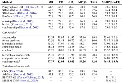
2005) andTREC(Li and Roth,2002). On all the datasets, we separately train a logistic regression model on top of the extracted sentence features. We restrict our comparison to methods that also aims to learn generic sentence embeddings for fair compar-ison. We also provide the state-of-the-art results us-ing task-dependent learnus-ing methods for reference. Results are summarized in Table3. Our CNN en-coder provides better results than the combine-skip model ofKiros et al.(2015) on all the 5 datasets.
We highlight some observations. First, the au-toencoder performs better than the future predic-tor, indicating that theintra-sentence information may be more important for classification than the
hierarchi-Method MR CR SUBJ MPQA TREC MSRP(Acc/F1)
ParagraphVec DM (Hill et al.,2016) 61.5 68.6 76.4 78.1 55.8 73.6 / 81.9 SDAE (Hill et al.,2016) 67.6 74.0 89.3 81.3 77.6 76.4 / 83.4 SDAE+emb. (Hill et al.,2016) 74.6 78.0 90.8 86.9 78.4 73.7 / 80.7 FastSent (Hill et al.,2016) 70.8 78.4 88.7 80.6 76.8 72.2 / 80.3 uni-skip (Kiros et al.,2015) 75.5 79.3 92.1 86.9 91.4 73.0 / 81.9 bi-skip (Kiros et al.,2015) 73.9 77.9 92.5 83.3 89.4 71.2 / 81.2 combine-skip (Kiros et al.,2015) 76.5 80.1 93.6 87.1 92.2 73.0 / 82.0 Our Results†
autoencoder 75.53 78.97 91.97 87.96 89.8 73.61 / 82.14
future predictor 72.56 78.44 90.72 87.48 86.6 71.87 / 81.68 hierarchical model 75.20 77.99 91.66 88.21 90.0 73.96 / 82.54 composite model 76.34 79.93 92.45 88.77 91.4 74.65 / 82.21
combine‡ 77.21 80.85 93.11 89.09 91.8 75.52 / 82.62
hierarchical model+emb. 75.30 79.37 91.94 88.48 90.4 74.25 / 82.70 composite model+emb. 77.16 80.64 92.14 88.67 91.2 74.88 / 82.28 combine+emb.‡ 77.77 82.05 93.63 89.36 92.6 76.45/83.76
Task-dependent methods
CNN (Kim,2014) 81.5 85.0 93.4 89.6 93.6 −
AdaSent (Zhao et al.,2015) 83.1 86.3 95.5 93.3 92.4 − Bi-CNN-MI (Yin and Schütze,2015) − − − − − 78.1/84.4
[image:7.595.102.494.64.329.2]MPSSM-CNN (He et al.,2015) − − − − − 78.6/84.7
Table 3: Classification accuracies on several standard benchmarks. The last column shows results on the task of paraphrase detection, where the evaluation metrics are classification accuracy and F1 score.†The first and second block in our results were obtained using the first and second method of considering words not in the training set, respectively. ‡“combine” means concatenating the feature vectors learned from both the hierarchical model and the composite model.
cal model performs better than the future predictor, demonstrating the importance of capturing long-term dependencies acrossmultiplesentences. Our combined model, which concatenates the feature vectors learned from both the hierarchical model and the composite model, performs the best. This may be due to that: (i) bothintra-and long-term
inter-sentence information are leveraged; (ii) it is easier to linearly separate the feature vectors in higher dimensional spaces. Further, using (fixed) pre-trained word embeddings consistently provides better performance than using the learned word embeddings. This may be due to thatword2vec
provides more generic word representations, since it is trained on the large Google News dataset (con-taining 100 billion words) (Mikolov et al.,2013).
To further demonstrate the advantage of the learned generic representations, we train a CNN classifier (i.e., a CNN encoder with a logistic regres-sion model on top) with two different initialization strategies: random initialization and initialization with trained parameters from the CNN-LSTM com-posite model. Results are shown in Figure3(left). The pretraining provides substantial improvements
MR CR SUBJ MPQA TREC Dataset 60
65 70 75 80 85 9095 100
Accuracy (%) PretrainRandom
10 20 30 40 50 60 70 80 90 Proportion (%) of labelled sentences 78
80 82 84 86 88 90 92 94
Accuracy (%) PretrainRandom
Figure 3: (Left) Effect of pretraining on the 5 clas-sification benchmarks. The error bars are over 10 different runs. (Right) Effect of pretraining on ac-curacy for the TREC dataset, in terms of change in the size of the labeled training set. The error bars are over 10 different samples of training sets. Pretraining means initializing the CNN parameters from the trained CNN-LSTM composite model.
[image:7.595.307.524.430.503.2]Image Annotation Image Search
Method R@1 Medr R@1 Medr
uni-skip† 30.6 3 22.7 4
bi-skip† 32.7 3 24.2 4
combine-skip† 33.8 3 25.9 4
Our Results
hierarchical model+emb. 32.7 3 25.3 4 composite model+emb. 33.8 3 25.7 4 combine+emb. 34.4 3 26.6 4
Task-dependent methods
DVSA∗ 38.4 1 27.4 3
[image:8.595.308.524.63.264.2]m-RNN‡ 41.0 2 29.0 3
Table 4: Results for image-sentence ranking ex-periments on the COCO dataset. R@Kdenotes Recall@K (higher is better) andMedris the me-dian rank (lower is better). (†) taken fromKiros et al.(2015). (∗) taken fromKarpathy and Fei-Fei
(2015). (‡) taken fromMao et al.(2015).
learning, with the autoencoder on all the data (la-beled and unlabled), and the classifier only on the labeled data.
Paraphrase detection Now we consider para-phrase detection on theMSRPdataset (Dolan et al.,
2004). On this task, one needs to predict whether or not two sentences are paraphrases. The training set consists of 4076 sentence pairs, and the test set has 1725 pairs. As inTai et al.(2015), given two sentence representationszxandzy, we first
com-pute their element-wise productzxzy and their
absolute difference|zx −zy|, and then
concate-nate them together. A logistic regression model is trained on top of the concatenated features to predict whether two sentences are paraphrases. We present our results on the last column of Table3. Our best result is better than the other results that use task-independent methods.
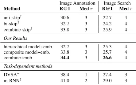
Image-sentence ranking We consider the task of image-sentence ranking, which aims to retrieve items in one modality given a query from the other. We use the COCO dataset (Lin et al.,2014), which contains 123,287 images each with 5 captions. For development and testing we use the same splits
asKarpathy and Fei-Fei(2015). The development
and test sets each contain 5000 images. We further split them into 5 random sets of 1000 images, and report the average performance over the 5 splits. Performance is evaluated using Recall@K, which measures the average times a correct item is found within the top-K retrieved results. We also report the median rank of the closest ground truth result
Method r ρ MSE
uni-skip† 0.8477 0.7780 0.2872
bi-skip† 0.8405 0.7696 0.2995
combine-skip† 0.8584 0.7916 0.2687
Our Results
autoencoder 0.8284 0.7577 0.3258 future predictor 0.8132 0.7342 0.3450 hierarchical model 0.8333 0.7646 0.3135 composite model 0.8434 0.7767 0.2972
combine 0.8533 0.7891 0.2791
hierarchical model+emb. 0.8352 0.7588 0.3152 composite model+emb. 0.8500 0.7867 0.2872 combine+emb. 0.8618 0.7983 0.2668
Task-dependent methods
Bi-LSTM‡ 0.8567 0.7966 0.2736
Tree-LSTM‡ 0.8676 0.8083 0.2532
Table 5: Results on the SICK semantic relatedness task. The evaluation metrics are Pearson’sr, Spear-man’sρand mean squared error (MSE). (†) taken fromKiros et al.(2015). (‡) taken fromTai et al.
(2015).
in the ranked list.
We represent images using 4096-dimensional feature vectors from VggNet (Simonyan and
Zis-serman, 2015). Each caption is encoded using
our trained CNN encoder. The training objec-tive is the same pairwise ranking loss as used
in Kiros et al. (2015), which takes the form of
max(0, α−f(xn, yn) +f(xn, ym)), wheref(·,·)
is the image-sentence score.(xn, yn)denotes the
related image-sentence pair, and(xn, ym) is the
randomly sampled unrelated image-sentence pair withn6=m. For image retrieval from sentences,x
denotes the caption,ydenotes the image, andvice versa. The objective is to force the matching score of the related pair(xn, yn)to be greater than the
unrelated pair(xn, ym)by a marginα, which is set
to 0.1 in our experiments.
Table4shows our results. Consistent with pre-vious experiments, we empirically found that the encoder trained using the fixed word embedding performed better on this task, hence only results using this method are reported. As can be seen, we obtain the same median rank as inKiros et al.
[image:8.595.70.292.65.204.2]re-trieving the most correct item than the skip-thought vector.
Semantic relatedness For our final experiment, we consider the task of semantic relatedness on the
SICKdataset (Marelli et al.,2014), consisting of 9927 sentence pairs. Given two sentences, our goal is to produce a real-valued score between [1,5]
to indicate how semantically related two sentences are, based on human generated scores. We compute a feature vector representing the pair of sentences in the same way as on the MSRP dataset. We follow the method inTai et al.(2015), and use the cross-entropy loss for training. Results are summarized in Table5. Our result is better than the combine-skip model ofKiros et al.(2015). This suggests that CNN also provides competitive performance at matching human relatedness judgements.
5 Conclusion
We presented a new class of CNN-LSTM encoder-decoder models to learn sentence representations from unlabeled text. Our trained convolutional encoder is highly generic, and can be an alternative to the skip-thought vectors ofKiros et al.(2015). Compelling experimental results on several tasks demonstrated the advantages of our approach. In future work, we aim to use more advanced CNN architectures (Conneau et al., 2016) for learning generic sentence embeddings.
Acknowledgments
This research was supported by ARO, DARPA, DOE, NGA, ONR and NSF.
References
Sanjeev Arora, Yingyu Liang, and Tengyu Ma. 2017. A simple but tough-to-beat baseline for sentence em-beddings. InICLR.
Frédéric Bastien, Pascal Lamblin, Razvan Pascanu, James Bergstra, Ian Goodfellow, Arnaud Bergeron, Nicolas Bouchard, David Warde-Farley, and Yoshua Bengio. 2012. Theano: new features and speed im-provements. arXiv:1211.5590.
Kyunghyun Cho, Bart Van Merriënboer, Caglar Gul-cehre, Dzmitry Bahdanau, Fethi Bougares, Holger Schwenk, and Yoshua Bengio. 2014. Learning phrase representations using rnn encoder-decoder for statistical machine translation. InEMNLP. Ronan Collobert, Jason Weston, Léon Bottou, Michael
Karlen, Koray Kavukcuoglu, and Pavel Kuksa. 2011.
Natural language processing (almost) from scratch. InJMLR.
Alexis Conneau, Holger Schwenk, Loïc Barrault, and Yann Lecun. 2016. Very deep convolu-tional networks for natural language processing.
arXiv:1606.01781.
Andrew M Dai and Quoc V Le. 2015. Semi-supervised sequence learning. InNIPS.
Bill Dolan, Chris Quirk, and Chris Brockett. 2004. Un-supervised construction of large paraphrase corpora: Exploiting massively parallel news sources. In COL-ING.
Zhe Gan, PD Singh, Ameet Joshi, Xiaodong He, Jianshu Chen, Jianfeng Gao, and Li Deng. 2017. Character-level deep conflation for business data an-alytics.arXiv preprint arXiv:1702.02640.
Jonas Gehring, Michael Auli, David Grangier, and Yann N Dauphin. 2016. A convolutional encoder model for neural machine translation.
arXiv:1611.02344.
Ian Goodfellow, Yoshua Bengio, and Aaron Courville. 2016.Deep Learning. MIT Press.
Hua He, Kevin Gimpel, and Jimmy J Lin. 2015. Multi-perspective sentence similarity modeling with con-volutional neural networks. InEMNLP.
Felix Hill, Kyunghyun Cho, and Anna Korhonen. 2016. Learning distributed representations of sentences from unlabelled data. InNAACL.
Sepp Hochreiter and Jürgen Schmidhuber. 1997. Long short-term memory. InNeural computation. Baotian Hu, Zhengdong Lu, Hang Li, and Qingcai
Chen. 2014. Convolutional neural network architec-tures for matching natural language sentences. In
NIPS.
Minqing Hu and Bing Liu. 2004. Mining and summa-rizing customer reviews. InSIGKDD.
Po-Sen Huang, Xiaodong He, Jianfeng Gao, Li Deng, Alex Acero, and Larry Heck. 2013. Learning deep structured semantic models for web search using clickthrough data. InCIKM.
Mohit Iyyer, Varun Manjunatha, Jordan L Boyd-Graber, and Hal Daumé III. 2015. Deep unordered composition rivals syntactic methods for text classi-fication. InACL.
Rie Johnson and Tong Zhang. 2015. Effective use of word order for text categorization with convolutional neural networks. InNAACL HLT.
Nal Kalchbrenner and Phil Blunsom. 2013. Recurrent continuous translation models. InEMNLP.
Andrej Karpathy and Li Fei-Fei. 2015. Deep visual-semantic alignments for generating image descrip-tions. InCVPR.
Yoon Kim. 2014. Convolutional neural networks for sentence classification. InEMNLP.
Diederik Kingma and Jimmy Ba. 2015. Adam: A method for stochastic optimization. InICLR.
Ryan Kiros, Yukun Zhu, Ruslan R Salakhutdinov, Richard Zemel, Raquel Urtasun, Antonio Torralba, and Sanja Fidler. 2015. Skip-thought vectors. In
NIPS.
Quoc Le and Tomas Mikolov. 2014. Distributed repre-sentations of sentences and documents. InICML.
Jiwei Li, Minh-Thang Luong, and Dan Jurafsky. 2015. A hierarchical neural autoencoder for paragraphs and documents. InACL.
Xin Li and Dan Roth. 2002. Learning question classi-fiers. InACL.
Rui Lin, Shujie Liu, Muyun Yang, Mu Li, Ming Zhou, and Sheng Li. 2015. Hierarchical recurrent neural network for document modeling. InEMNLP.
Tsung-Yi Lin, Michael Maire, Serge Belongie, James Hays, Pietro Perona, Deva Ramanan, Piotr Dollár, and C Lawrence Zitnick. 2014. Microsoft coco: Common objects in context. InECCV.
Zhouhan Lin, Minwei Feng, Cicero Nogueira dos San-tos, Mo Yu, Bing Xiang, Bowen Zhou, and Yoshua Bengio. 2017. A structured self-attentive sentence embedding. InICLR.
Junhua Mao, Wei Xu, Yi Yang, Jiang Wang, Zhiheng Huang, and Alan Yuille. 2015. Deep captioning with multimodal recurrent neural networks (m-rnn). InICLR.
Marco Marelli, Luisa Bentivogli, Marco Baroni, Raf-faella Bernardi, Stefano Menini, and Roberto Zam-parelli. 2014. Semeval-2014 task 1: Evaluation of compositional distributional semantic models on full sentences through semantic relatedness and textual entailment. SemEval-2014.
Fandong Meng, Zhengdong Lu, Mingxuan Wang, Hang Li, Wenbin Jiang, and Qun Liu. 2015. Encod-ing source language with convolutional neural net-work for machine translation. InACL.
Tomas Mikolov, Martin Karafiát, Lukas Burget, Jan Cernock`y, and Sanjeev Khudanpur. 2010. Recurrent neural network based language model. In INTER-SPEECH.
Tomas Mikolov, Ilya Sutskever, Kai Chen, Greg S Cor-rado, and Jeff Dean. 2013. Distributed representa-tions of words and phrases and their compositional-ity. InNIPS.
Jeff Mitchell and Mirella Lapata. 2010. Composition in distributional models of semantics.Cognitive sci-ence.
Matteo Pagliardini, Prakhar Gupta, and Martin Jaggi. 2017. Unsupervised learning of sentence em-beddings using compositional n-gram features.
arXiv:1703.02507.
Bo Pang and Lillian Lee. 2004. A sentimental educa-tion: Sentiment analysis using subjectivity summa-rization based on minimum cuts. InACL.
Bo Pang and Lillian Lee. 2005. Seeing stars: Exploit-ing class relationships for sentiment categorization with respect to rating scales. InACL.
Yelong Shen, Xiaodong He, Jianfeng Gao, Li Deng, and Grégoire Mesnil. 2014. A latent semantic model with convolutional-pooling structure for information retrieval. InCIKM.
Karen Simonyan and Andrew Zisserman. 2015. Very deep convolutional networks for large-scale image recognition. InICLR.
Richard Socher, Eric H Huang, Jeffrey Pennington, An-drew Y Ng, and Christopher D Manning. 2011. Dy-namic pooling and unfolding recursive autoencoders for paraphrase detection. InNIPS.
Richard Socher, Alex Perelygin, Jean Y Wu, Jason Chuang, Christopher D Manning, Andrew Y Ng, and Christopher Potts. 2013. Recursive deep mod-els for semantic compositionality over a sentiment treebank. InEMNLP.
Alessandro Sordoni, Yoshua Bengio, Hossein Vahabi, Christina Lioma, Jakob Grue Simonsen, and Jian-Yun Nie. 2015. A hierarchical recurrent encoder-decoder for generative context-aware query sugges-tion. InCIKM.
Nitish Srivastava, Geoffrey E Hinton, Alex Krizhevsky, Ilya Sutskever, and Ruslan Salakhutdinov. 2014. Dropout: a simple way to prevent neural networks from overfitting. JMLR.
Nitish Srivastava, Elman Mansimov, and Ruslan Salakhudinov. 2015. Unsupervised learning of video representations using lstms. InICML.
Ilya Sutskever, Oriol Vinyals, and Quoc V Le. 2014. Sequence to sequence learning with neural networks. InNIPS.
Kai Sheng Tai, Richard Socher, and Christopher D Manning. 2015. Improved semantic representations from tree-structured long short-term memory net-works. InACL.
Janyce Wiebe, Theresa Wilson, and Claire Cardie. 2005. Annotating expressions of opinions and emo-tions in language. InLanguage resources and evalu-ation.
John Wieting, Mohit Bansal, Kevin Gimpel, and Karen Livescu. 2016. Towards universal paraphrastic sen-tence embeddings. InICLR.
Wenpeng Yin and Hinrich Schütze. 2015. Convolu-tional neural network for paraphrase identification. InHLT-NAACL.
Mo Yu and Mark Dredze. 2015. Learning composition models for phrase embeddings. TACL.
Xiang Zhang, Junbo Zhao, and Yann LeCun. 2015. Character-level convolutional networks for text clas-sification. InNIPS.
Han Zhao, Zhengdong Lu, and Pascal Poupart. 2015. Self-adaptive hierarchical sentence model.
arXiv:1504.05070.