http://wrap.warwick.ac.uk
Original citation:
Wang, Kai, Lin, Minghong, Ciucu, Florin, Wierman, Adam and Lin, Chuang. (2015)
Characterizing the impact of the workload on the value of dynamic resizing in data
centers. Performance Evaluation, Volume 85-86 . pp. 1-18.
Permanent WRAP url:
http://wrap.warwick.ac.uk/69946
Copyright and reuse:
The Warwick Research Archive Portal (WRAP) makes this work by researchers of the
University of Warwick available open access under the following conditions. Copyright ©
and all moral rights to the version of the paper presented here belong to the individual
author(s) and/or other copyright owners. To the extent reasonable and practicable the
material made available in WRAP has been checked for eligibility before being made
available.
Copies of full items can be used for personal research or study, educational, or
not-for-profit purposes without prior permission or charge. Provided that the authors, title and
full bibliographic details are credited, a hyperlink and/or URL is given for the original
metadata page and the content is not changed in any way.
Publisher’s statement:
© 2015, Elsevier. Licensed under the Creative Commons
Attribution-NonCommercial-NoDerivatives 4.0 International http://creativecommons.org/licenses/by-nc-nd/4.0/
A note on versions:
The version presented here may differ from the published version or, version of record, if
you wish to cite this item you are advised to consult the publisher’s version. Please see
the ‘permanent WRAP url’ above for details on accessing the published version and note
that access may require a subscription.
.
Characterizing the Impact of the Workload on
the Value of Dynamic Resizing in Data Centers
IKai Wanga,∗, Minghong Linb, Florin Ciucuc, Adam Wiermand, Chuang Lind
aState Key Laboratory of Computer Science, Institute of Software, Chinese Academy of Sciences, China bFacebook, USA
cComputer Science Department, University of Warwick, UK
dDept. of Computing and Mathematical Sciences, California Institute of Technology, USA eDept. of Computer Science and Technology, Tsinghua University, China
Abstract
Energy consumption imposes a significant cost for data centers; yet much of that energy is used to maintain excess service capacity during periods of predictably low load. Resultantly, there has recently been interest in developing designs that allow the service capacity to be dynamically resized to match the current workload. However, there is still much debate about the value of such approaches in real settings. In this paper, we show that the value of dynamic resizing is highly dependent on statistics of the workload process. In particular, both slow time-scale non-stationarities of the workload (e.g., the peak-to-mean ratio) and the fast time-scale stochasticity (e.g., the burstiness of arrivals) play key roles. To illustrate the impact of these factors, we combine optimization-based modeling of the slow time-scale with stochastic modeling of the fast time-scale. Within this framework, we provide both analytic and numerical results characterizing when dynamic resizing does (and does not) provide benefits.
Keywords: Data Centers, Dynamic Resizing, Energy Efficient IT, Stochastic Network Calculus
1. Introduction
Energy costs represent a significant, and growing, fraction of a data center’s budget. Hence there is a push to improve the energy efficiency of data centers, both in terms of the components (servers, disks, network, power infrastructure [3, 4, 5, 6, 7]) and the algorithms [8, 9, 10, 11, 12]. One specific aspect of data center design that is the focus of this paper is dynamically resizing the service capacity of the data center so that during periods of low load some servers are allowed to enter a power-saving mode (e.g., go to sleep or shut down).
The potential benefits of dynamic resizing have been a point of debate in the community [13, 9, 14, 15, 16]. On one hand, it is clear that, because data centers are far from perfectly energy proportional, significant energy is used to maintain excess capacity during periods of predictably low load when there is a diurnal workload with a high peak-to-mean ratio. On the other hand, there are also significant costs to dynamically adjusting the number of active servers. These costs come in terms of the engineering challenges in making this possible [17, 18, 19], as well as the latency, energy, and wear-and-tear costs of the actual “switching” operations involved [20, 9, 21].
The challenges for dynamic resizing highlighted above have been the subject of significant research. At this point, many of the engineering challenges associated with facilitating dynamic resizing have been resolved, e.g., [17, 18, 19].
IThis paper is the full version of an accepted poster at ACM Sigmetrics/Performance 2012 [1] and an accepted short paper at the IEEE Infocom
2013 conference [2]
∗Corresponding author. Tel.:+86 138 1049 1901.
Email addresses:[email protected](Kai Wang),[email protected](Minghong Lin),[email protected](Florin Ciucu),
Additionally, the algorithmic challenge of deciding, without knowledge of the future workload, whether to incur the significant “switching costs” associated with changing the available service capacity has been studied in depth and a number of promising algorithms have emerged [11, 22, 9, 23, 12].
However, despite this body of work, the question of characterizing the potential benefits of dynamic resizing has still not been properly addressed. Providing new insight into this topic is the goal of the current paper.
The perspective of this paper is that, apart from engineering challenges, the key determinant of whether dynamic resizing is valuable is the workload, and that proponents on different sides tend to have different assumptions in this regard. In particular, a key observation, which is the starting point for our work, is that there are two factors of the workload which provide dynamic resizing potential savings:
(i) Non-stationarities at a slow time-scale, e.g., diurnal workload variations.
(ii) Stochastic variability at a fast time-scale, e.g., the burstiness of request arrivals.
The goal of this work is to investigate the impact of and interaction between these two features with respect to dynamic resizing.
To this point,we are not aware of any work characterizing the benefits of dynamic resizing that captures both of these features. There is one body of literature which provides algorithms that take advantage of (i), e.g., [9, 10, 11, 22, 24, 25, 16]. This work tends to use an optimization-based approach to develop dynamic resizing algorithms. There is another body of literature which provides algorithms that take advantage of (ii), e.g., [23, 21]. This work tends to assume a stationary queueing model with Poisson arrivals to develop dynamic resizing algorithms.
The first contribution of the current paper is to provide an analytic framework that captures both effects (i) and (ii). We accomplish this by using an optimization framework at the slow time-scale (see Section 2), which is similar to that of [11], and combining this with stochastic network calculus and large deviations modeling for the fast time-scale (see Section 3), which allows us to study a wide variety of underlying arrival processes. We consider both light-tailed models with various degrees of burstiness and heavy-tailed models that exhibit self-similarity. The interface between the fast and slow time-scale models happens through a constraint in the optimization problem that captures the Service Level Agreement (SLA) for the data center, which is used by the slow time-scale model but calculated using the fast time-scale model (see Section 3).
Using this modeling framework, we are able to provide both analytic and numerical results that yield new insight into the potential benefits of dynamic resizing (see Section 4). Specifically, we use trace-driven numerical simulations to study (i) the role of burstiness for dynamic resizing, (ii) the role of the peak-to-mean ratio for dynamic resizing, (iii) the role of the SLA for dynamic resizing, and (iv) the interaction between (i), (ii), and (iii). The key realization is that each of these parameters are extremely important for determining the value of dynamic resizing. In particular, for any fixed choices of two of these parameters, the third can be chosen so that dynamic resizing does or does not provide significant cost savings for the data center. Thus, performing a detailed study of the interaction of these factors is important. To that end, Figures 12-14 provide concrete illustrations of which settings of peak-to-mean ratio, burstiness, and SLAs dynamic resizing is and is not valuable. Hence, debate about thepotentialvalue of dynamic resizing can be transformed into debate about characteristics of the workload and the SLA.
There are some interesting facts about these parameters individually that our case studies uncover. Two important examples are the following. First, while one might expect that increased burstiness provides increased opportunities for dynamic resizing, it turns out the burstiness at the fast time-scale actually reduces the potential cost savings achievable via dynamic resizing. The reason is that dynamic resizing necessarily happens at the slow time-scale, and so the increased burstiness at the fast time-scale actually results in the SLA constraint requiringmoreservers be used at the slow time-scale due to the possibility of a large burst occurring. Second, it turns out the impact of the SLA can be quite different depending on whether the arrival process is heavy- or light-tailed. In particular, as the SLA becomes more strict, the cost savings possible via dynamic resizing under heavy-tailed arrivals decreases quickly; however, the cost savings possible via dynamic resizing under light-tailed workloads is unchanged.
In addition to detailed case studies, we provide analytic results that support many of the insights provided by the numerics. In particular, Theorems 1 and 2 provide monotonicity and scaling results for dynamic resizing in the case of Poisson arrivals and heavy-tailed, self-similar arrivals.
and analyzes the impact different arrival models have on the SLA constraint of the dynamic resizing algorithm used in the slow time-scale. Then, Section 4 provides case studies and analytic results characterizing the impact of the workload on the benefits of dynamic resizing. The related proofs are presented in Section 5. Finally, Section 6 provides concluding remarks.
2. Slow Time-scale Model
In this section and the one that follows, we introduce our model. We start with the “slow time-scale model”. This model is meant to capture what is happening at the time-scale of the data center control decisions, i.e., at the time-scale which the data center is willing to adjust its service capacity. For many reasons, this is a much slower time-scale than the time-scale at which requests arrive to the data center. We provide a model for this “fast time-scale” in the next section.
The slow time-scale model parallels closely the model studied in [11]. The only significant change is to add a constraint capturing the SLA to the cost optimization solved by the data center. This is a key change, which allows an interface to the fast time-scale model.
2.1. The Workload
At this time-scale, our goal is to provide a model which can capture the impact of diurnal non-stationarities in the workload. To this end, we consider a discrete-time model such that there is a time interval of interest which is evenly divided into “frames”k∈ {1, ...,K}. In practice, the length of a frame could be on the order of 5-10 minutes, whereas the time interval of interest could be as long as a month/year. The mean request arrival rate to the data center in framekis denoted byλk, and non-stationarities are captured by allowing different rates during different frames.
Although we could allowλkto have a vector value to represent more than one type of workload as long as the resulting
cost function is convex in our model, we assumeλkto have a scalar value in this paper to simplify the presentation.
Because the request inter-arrival times are much shorter than the frame length, typically in the order of 1-10 seconds, capacity provisioning can be based on the average arrival rate during a frame.
2.2. The Data Center Cost Model
The model for data center costs focuses on the server costs of the data center, as minimizing server energy con-sumption also reduces cooling and power distribution costs. We model the cost of a server by the operating costs incurred by an active server, as well as the switching cost incurred to toggle a server into and out of a power-saving model (e.g., off/on or sleeping/waking). Both components can be assumed to include energy cost, delay cost, and wear-and-tear cost. The model framework we adopt is fairly standard and has been used in a number of previous papers, e.g., see [11, 26] for a further discussion of the work and [27] for a discussion of how the model relates to implementation challenges.
Note that this model ignores many issues surrounding reliability and availability, which are key components of data center service level agreements (SLAs). In practice, a solution that toggles servers must still maintain the reliability and availability guarantees; however this is beyond the scope of the current paper. See [18] for a discussion.
The Operating Cost
The operating costs are modeled by a convex function f(λi,k), which is the same for all the servers, whereλi,k
denotes the average arrival rate to serveriduring framek. The convexity assumption is quite general and captures many common server models. One example, which we consider in our numeric examples later, is to say that the operating costs are simply equal to the energy cost of the server, i.e., the energy cost of an active server handling arrival rateλi,k. This cost is often modeled using an affine function as follows
f(λi,k)=e0+e1λi,k, (1)
The Switching Cost
The switching cost, denoted byβ, models the cost of toggling a server back-and-forth between active and power-saving models. The switching cost includes the costs of the energy used toggling a server, the delay in migrating connections/data when toggling a server, and the increased wear-and-tear on the servers toggling.
2.3. The Data Center Optimization
Given the cost model above, the data center has two control decisions at each time: determiningnk, the number of
active servers in every time frame, and assigning arriving jobs to servers, i.e., determiningλi,ksuch thatΣin=k1λi,k=λk.
All servers are assumed to be homogeneous with constant rate capacityµ > 0. Modeling heterogeneous servers is possible but the online problem will become more complicated [26] , which is out of the scope of this paper.
The goal of the data center is to determinenkandλi,kto minimize the cost incurred during [0,K], which is modeled
as follows:
min
K
X
k=1
nk X
i=1
f(λi,k)+β K
X
k=1
(nk−nk−1)+ (2)
s.t.
0≤λi,k≤λk
Σnk
i=1λi,k=λk P(Dk>D¯)≤ε ,¯
(3)
where the final constraint is introduced to capture the SLA of the data center. We useDkto represent the steady-state
delay during framek, and ( ¯D,¯) to represent an SLA of the form “the probability of a delay larger than ¯Dmust be bounded by probability ¯ε”.
This model generalizes the data center optimization problem from [11] by accounting for the additional SLA constraint. The specific values in this constraint are determined by the stochastic variability at the fast time-scale. In particular, we derive (for a variety of workload models) a sufficient constraintnk≥Ck( ¯µD,¯ε) such that
nk≥
Ck( ¯D,ε¯)
µ =⇒P(Dk>D¯)≤ε .¯ (4)
Here,µis the constant rate capacity of each server andCk( ¯D,ε¯) is to be determined for each considered arrival model.
One should interpretCk( ¯D,ε¯) as the overall effective capacity/bandwidth needed in the data center such that the SLA
delay constraint is satisfied within framek.
Note that the new constraint is only sufficient for the original SLA constraint. The reason is thatCk( ¯D,ε¯) will be
computed, in the next section, from upper bounds on the distribution of the transient delay within a frame.
With the new constraint, however, the optimization problem in (2)-(3) can be considerably simplified. Indeed, note thatnkis fixed during each time framekand the remaining optimization forλi,kis convex. Thus, we can simplify
the form of the optimization problem by using the fact that the optimal dispatching strategyλ∗
i,kis load balancing, i.e.,
λ∗ 1,k=λ
∗
2,k=. . .=λk/nk. This decouples dispatchingλ∗i,kfrom capacity planningnk, and so Eqs. (2)-(3) become:
Data Center Optimization Problem
min
K
X
k=1
nkf(λk/nk)+β K
X
k=1
(nk−nk−1)+ (5)
s.t.nk≥
Ck( ¯D,ε¯)
µ .
Note that (5) is a convex optimization, sincenkf(λk/nk) is the perspective function of the convex function f(·).
2.4. Algorithms for Dynamic Resizing
Though the Data Center Optimization Problem described above is convex, in practice it must be solvedonline, i.e., without knowledge of the future workload. Thus, in determiningnk, the algorithm may not have access to the
future arrival ratesλlforl>k. This fact makes developing algorithms for dynamic resizing challenging. However,
progress has been made recently [11, 30].
Deriving algorithms for this problem is not the goal of the current paper. Thus, we make use of a recent algorithm called Lazy Capacity Provisioning (LCP) [11]. We choose LCP because of the strong analytic performance guarantees it provides – LCP provides cost within a factor of 3 of optimal for any (even adversarial) workload process.
LCP works as follows. Let (nL k,1, . . . ,n
L
k,k) be the solution vector to the following optimization problem
min
k
X
l=1
nlf(λl/nl)+β k
X
l=1
(nl−nl−1)+
s.t.nl≥
Cl( ¯D,ε¯)
µ , n0=0.
Similarly, let (nU k,1, . . . ,n
U
k,k) be the solution vector to the following optimization problem
min
k
X
l=1
nlf(λl/nl)+β k
X
l=1
(nl−1−nl)+
s.t.nl≥
Cl( ¯D,ε¯)
µ , n0=0.
Denote (n)b
a =max(min(n,b),a) as the projection ofninto the closed interval [a,b]. Then LCP can be defined using nL
k,kandn U
k,kas follows. Informally, LCP stays “lazily” between the upper boundn U
k,kand the lower boundn L k,kin all
frames.
Lazy Capacity Provisioning, LCP
Let nLCP=(nLCP
0 , . . . ,n
LCP
K )denote the vector of active servers under LCP. This vector can be calculated online using the following forward recurrence relation:
nLCPk =
0, k≤0
(nLCP k−1)
nU k,k
nL k,k, 1
≤k≤K.
Note that, in [11], LCP is introduced and analyzed for the optimization from Eq. (5) without the SLA constraint. However, it is easy to see that the algorithm and performance guarantee extend to our setting. Specifically, the guarantees on LCP hold in our setting because the SLA constraint can be removed by defining the operating cost to be∞instead ofnkf(λk/nk) whennk<Ck( ¯D,ε¯)/µ.
A last point to highlight about LCP is that, as described, it does not use any predictions about the workload in future frames. Such information could clearly be beneficial, and can be incorporated into LCP if desired, see [11].
3. Fast Time-scale Model
Given the model of the slow time-scale in the previous section, we now zoom in to give a description for the fast time-scale model. By “fast” time-scale, we mean the time-scale at which requests arrive, e.g., on the order of 1-10 seconds, as opposed to the “slow” time-scale (frame length) at which dynamic resizing decisions are made by the data center e.g., on the order of 5-15 minutes. To model the fast time-scale, we evenly break each frame from the slow time-scale into “slots”t∈ {1, . . . ,U}, such that frame length=U·slot length.
The goal of this section is to derive the value ofCk( ¯D,ε¯) in the constraintnk ≥ Ck( ¯µD,¯ε) from Eq. (4), and thus
enable an interface between the fast and slow time-scales by parameterizing the Data Center Optimization Problem from Eq. (5) for a broad range of workloads.
Note that throughout this section we suppress frame’s subscriptkfornk,λk,Ck, andDk, and focus on a generic
frame.
Our approach for deriving the SLA constraint for the Data Center Optimization Problem will be to first derive an “aggregation property” which allows the data center to be modeled as a single server, and to then derive bounds on the distribution of the transient delay under a variety of arrival processes.
Note that, in this paper, for simplicity of exposition, the arrival and server models in the fast time-scale have been defined such that stationary increments are implicitly assumed. This is a mild assumption given the length of frames defined by the slow time-scale, and is satisfied by the traces used in Section 4. However, if one would like to study non-stationary processes, the results in this paper can be extended. The resulting bounding functions will generally be dynamic and time-dependent.
3.1. An Aggregation Property
To get intuition for the aggregation property we prove, observe that if the arrival process were modeled as Poisson and job sizes were exponential, then an “aggregation property” would be immediate, since the response time distribu-tion only depends on the load. Hence the SLA could be derived by considering a single server. Outside of this simple case, however, we need to derive a suitable single server approximation.
The aggregation result that we derive and apply is formulated in the framework of stochastic network calculus [31], and so we begin by briefly introducing this framework.
Denote the cumulative arrival (workload) process at the data center’s dispatcher by A(t). That is, for each slot
t =1, . . . ,U,A(t) counts the total number of jobs arrived in the time interval [0,t]. Depending on the total number
nof active servers, the arrival process is dispatched into the sub-arrival processesAi(t) withi =1, . . . ,nsuch that A(t)=P
iAi(t). The cumulative response processes from the servers are denoted byRi(t), whereas the total cumulative
response process from the data center is denoted byR(t)=P
iRi(t). All arrival and response processes are assumed
to be non-negative, non-decreasing, and left-continuous, and satisfy the initial condition A(0) = R(0) = 0. For convenience we use the bivariate extensionsA(s,t) :=A(t)−A(s) andR(s,t) :=R(t)−R(s).
The service provided by a server is modeled in terms of probabilistic lower bounds using the concept of a stochastic service process. This is a bivariate random processS(s,t) which is non-negative, non-decreasing, and left-continuous. Formally, a server is said to guarantee a (stochastic) service processS(s,t) if foranyarrival processA(t) the corre-sponding response processR(t) from the server satisfies for allt≥0
R(t)≥A∗S(t), (6)
where ‘∗’ denotes the min-plus convolution operator, i.e., for two (random) processesA(t) andS(s,t),
A∗S(t) := inf 0≤s≤t
{A(s)+S(s,t)} . (7)
The inequality in (6) is assumed to hold almost surely. Note that the lower bound set by the service process is invariant to the arrival processes.
We are now ready to state the aggregation property. The proof is deferred to Section 5.
Lemma 1. Consider an arrival process A(t)which is dispatched to n servers. Each server i is work-conserving with constant rate capacityµ > 0. Arrivals are dispatched deterministically across the servers such that each server i receives a fraction 1n of the arrivals. Then, the system has service process S(s,t)=nµ(t−s),i.e., R(t)≥A∗S(t).
0 100 200 300 400 500 600 0
200 400 600 800 1000
time slot (1 sec)
instantaneous arrival rate
heavy−tailed MM
[image:8.595.114.481.119.252.2]Poisson
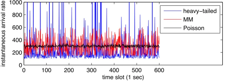
Figure 1: Three synthetically generated traces within 1 frame, withλ=300 of Poisson, Markov-Modulated (MM) (T=1,λl=0.5λandλh=2λ),
and heavy-tailed arrivals (b=λ/3 andα=1.5).
3.2. Arrival Processes
Now that we can reduce the study of the multi-server system to the study of a single server system using Lemma 1, we can move to characterizing the impact of the arrival process on the SLA constraint in the Data Center Optimization Problem.
In particular, the next step in deriving the SLA constraintn≥ C( ¯Dµ,¯ε) is to derive a bound on the distribution of the delay at the virtual server with arrival processA(t) and service processS(s,t)=C( ¯D,ε¯)(t−s), i.e.,
P
D(t)>D¯≤ε( ¯D). (8)
It is important to observe that the violation probabilityεholds for thetransient virtualdelay processD(t), which is defined asD(t) := inf{d:A(t−d)≤R(t)}, and which models the delay spent in the system by the job leaving the system, if any, at timet. By this definition, and using the servers’ homogeneity and also the deterministic splitting of arrivals from Lemma 1, the virtual delay for the aggregate virtual server is the same as the virtual delay for the individual servers. This fact guarantees that an SLA constraint on the virtual server implicitly holds for the individual servers as well. Moreover, the violation probabilityεin Eq. (8) is derived so that it is time invariant, which implies that it bounds the distribution of the stead-state delayD=limt→∞D(t) as well. Therefore, the value ofC( ¯D,ε¯) can be finally computed by solving the implicit equationε( ¯D)=ε¯.
In the following, we follow the outline above to computeC( ¯D,ε¯) for light- and heavy-tailed arrival processes. Interested readers may refer to the technical report [32] for details. Figure 1 depicts examples of the three types of arrival processes we consider in 1 frame: Poisson, Markov-Modulated (MM), and heavy-tailed arrivals. In all three cases, the mean arrival rate isλ = 300. The figure clearly illustrates the different levels of burstiness of the three traces.
3.2.1. Light-tailed Arrivals
We consider two examples of light-tailed arrival processes: Poisson and Markov-Modulated (MM) processes.
Poisson Arrivals
We start with the case of Poisson processes, which are characterized by a low level of burstiness, due to the independent increments property. The following proposition, providing the tail of the virtual delay, is a minor variation of a result from [33]; for the proof see [32].
Proposition 1. Let A(t)be a Poisson process with some rateλ >0, and define
θ∗:=supθ >0 : λ
θ
eθ−1≤C( ¯D,ε¯)
Then a bound on the transient delay process is given for all t≥0by
P
D(t)>D¯≤e−θ∗C( ¯D,¯ε) ¯D:=ε( ¯D). (10)
Solving forC( ¯D,ε¯) by setting the violation probabilityε( ¯D) equal to ¯εyields the implicit solution
C( ¯D,ε¯)=− 1
θ∗D¯ log ¯ε .
Further, using the monotonicity of the function λθeθ−1inθ >0 we immediately get the explicit solution
C( ¯D,ε¯)= K
log (1+K)λ , (11)
where
K=−log ¯ε
λD¯ .
Markov-Modulated Arrivals
Consider now the case of Markov-Modulated (MM) processes which, unlike the Poisson processes, do not nec-essarily have independent increments. The key feature for the purposes of this paper is that the burstiness of MM processes can be arbitrarily adjusted.
We consider a simple MM processes with two states. Let a discrete and homogeneous Markov chain x(s) with two states denoted by ‘low’ and ‘high’, and transition probabilitiesphandplbetween the ‘low’ and ‘high’ states, and
vice-versa, respectively. Assuming that a source produces at some constant ratesλl>0 andλh > λlwhile the chain x(s) is in the ‘low’ and ‘high’ states, respectively, then the corresponding MM cumulative arrival process is
A(t)=
t
X
s=1
λlI{x(s)=‘low0}+λhI{x(s)=‘high0}
, (12)
whereI{·}is the indicator function. The average rate ofA(t) isλ=
pl
ph+plλl+
ph
ph+plλh. To adjust the burstiness level ofA(t) we introduce the parameterT := p1
h + 1
pl, which is the average time for the Markov chainx(s) to change states twice. We note that the higher the value ofT is, the higher the burstiness level becomes (the time periods whilst x(s) spends in the ‘high’ or ‘low’ states get longer and longer).
To compute the delay bound let us construct the matrix
Ψ(θ)= (1−ph)e
θλl p
heθλh pleθλl (1−pl)eθλh
!
,
for someθ >0 and consider its spectral radius
λ(θ) :=(1−ph)e
θλl+(1−p
l)eθλh+
√ ∆
2 , (13)
where∆ =(1−ph)eθλl−(1−pl)eθλh
2
+4phpleθ(λl+λh). Let also
K(θ) :=max
(
pheθλh
λ(θ)−(1−ph)eθλl
,λ(θ)−(1−ph)eθλl pheθλh
)
. (14)
The two terms are the ratios of the elements of the right-eigenvector of the matrixΨ(θ). Also, let
θ∗:=sup
(
θ >0 : 1
θlogλ(θ)≤C( ¯D,ε¯)
)
.
Proposition 2. Consider a MM cumulative arrival process as defined in (12), with theλ(θ)given in (13), and K(θ)
given in (14), then a bound on the transient delay process is
P
D(t)>D¯≤K(θ∗)e−θ∗C( ¯D,¯ε) ¯D:=ε( ¯D).
Setting the violation probabilityε( ¯D) equal to ¯εin Theorem 2 yields the implicit solution
C( ¯D,ε¯)=− 1
θ∗D¯ log ¯
ε
K(θ∗) . (15)
3.3. Heavy-tailed and Self-similar Arrivals
We now consider the class of heavy-tailed and self-similar arrival processes. These processes are fundamentally different from light-tailed processes in that deviations from the mean increase in time and decay in probability as a power law, i.e., more slower than the exponential.
We consider in particular the case of a source generating jobs in every slot according to i.i.d. Pareto random variablesXiwith tail distribution for allx≥b:
P(Xi>x)=(x/b)−α, (16)
where 1 < α <2. X has finite meanE[X] =αb/(α−1) and infinite variance. For the corresponding bound on the transient delay we reproduce a result from [34].
Proposition 3. Consider a source generating jobs in every slot according to i.i.d. Pareto random variables Xi, with the tail distribution from (16). The bound on the transient delay is
P
D(t)>D¯≤KC( ¯D,ε¯) ¯D1−α:=ε( ¯D), (17)
where
K= inf 1<γ<C( ¯D,¯ε)
λ
C( ¯D,ε¯)
γ −λ
!−1 αγα−1α
(α−1) logγ
.
Setting the violation probabilityε( ¯D) equal to ¯ε, we get the implicit solution
inf 1<γ<C( ¯D,¯ε)
λ
γ
C( ¯D,ε¯)α−1C( ¯D,ε¯)−γλ
γα−1 α
logγα−1α
=ε¯D¯α−1. (18)
4. Case Studies
Given the model described in the previous two sections, we are now ready to explore the potential of dynamic resizing in data centers, and how this potential depends on the interaction between non-stationarities at the slow time-scale and burstiness/self-similarity at the fast time-scale. Our goal in this section is to provide insight into which workloads dynamic resizing is valuable for. To accomplish this, we provide a mixture of analytic results and trace-driven numerical simulations in this section.
It is important to note that the case studies that follow depend fundamentally on the modeling performed so far in the paper, which allows us to capture and adjust independently, both fast time-scale and slow time-scale properties of the workload. The generality of our model framework enables thus a rigorous study of the impact of the workload on value of dynamic resizing.
4.1. Setup
0 50 100 150 200 250 0
200 400 600 800 1000
Arrival
Time frame k (10 mins)
(a) Hotmail
0 100 200 300 400 500 600 700
0 200 400 600 800 1000
Arrival
Time frame k (10 mins)
[image:11.595.74.528.110.209.2](b) MSR
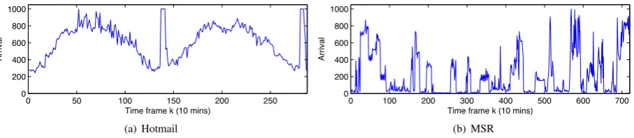
Figure 2: Illustration of the traces used for numerical experiments.
Model Parameters
The time frame for adapting the number of serversnkis assumed to be 10 min, and each time slot is assumed to
be 1 s, i.e.,U = 600. When not otherwise specified, we assume the following parameters for the data centerS LA
agreement: the (virtual) delay upper bound ¯D=200ms, and the delay violation probability ¯ε=10−3.
The cost is characterized by the two parameters ofe0ande1, and the switching costβ. We choose units such that the fixed energy cost ise0=1. The load-dependent energy consumption is set toe1=0, because the energy consumption of current servers with typical utilization level is dominated by the fixed costs [28, 4, 29]. Note that adjustinge0and
e1changes the magnitude of potential savings under dynamic resizing, but does not affect the qualitative conclusions about the impact of the workload. So, due to space constraints, we fix these parameters during the case studies.
The normalized switching costβ/e0measures the duration a server must be powered down to outweigh the switch-ing cost. Unless otherwise specified, we useβ=6, which corresponds to the energy consumption for one hour (six frames). This was chosen as an estimate of the time a server should sleep so that the wear-and-tear of power cycling matches that of operating [20, 11].
Workload Information
For the slow time-scale, i.e.,λk, the workloads are drawn from two real-world data center traces. The first set of
traces is from Hotmail, a large email service running on tens of thousands of servers. We used traces from 8 such servers over a 48-hour period, starting at midnight (PDT) on Monday August 4 2008 [18]. The second set of traces is taken from 6 RAID volumes at MSR Cambridge. The traced period was 1 week starting from 5PM GMT on the 22nd February 2007 [18]. Thus, these activity traces represent a service used by millions of users and a small service used by hundreds of users.
The original load is averaged over each frame, on the order of 10 minutes, and the traces are normalized as peak loadλpeak=1000, which are visualized in Figure 2. Both sets of traces show strong diurnal properties and have
peak-to-mean ratios (PMRs) of 1.64 and 4.64 for Hotmail and MSR respectively. The traces are then used as the values ofλk in the corresponding framek. We also adjust the peak-to-mean ratio for some experiments by scalingλk as
ˆ
λk=c(λk)γ, varyingγand adjustingcto keep the mean constant. In this way, we can simulate a variety of realistic
arrival processes with discrete-event simulation for the optimization problem (Eq. (5)), fix a cost function, and then use a scheduling algorithm for the slow time-scale, at each time step using the fast time-scale as input.
To simulate the stochastic burstiness of the workload at the fast time-scale model, at each time step for the opti-mization problem (Eq. (5)), we adapt the workload based on the mean arrival rate in each frame (λk) to parameterize
the arrival processes,A(t). For the stochastic processes being simulated, we consider two examples of light-tailed ar-rival processes: Poisson and Markov-Modulated (MM) processes, as well as the class of heavy-tailed and self-similar arrival processes. To parameterize the MM processes, we takeλl=.5λ,λh=2λ, and we adjust the burst parameterT
0 50 100 150 200 250 300 350 0
500 1000 1500 2000 2500
time frame k (10 mins)
number of servers n
k
=1.1 =1.3 =1.5 =1.7 =1.9 Poisson
(a) Hotmail
0 100 200 300 400 500 600 700 800 900
0 500 1000 1500 2000 2500
time frame k (10 mins)
number of servers n
k
_=1.1
_=1.3
_=1.5
_=1.7
_=1.9
Poisson
[image:12.595.67.526.110.349.2](b) MSR
Figure 3: Impact of burstiness on provisioningnkfor heavy-tailed arrivals.
0 50 100 150 200 250 300 350
0 500 1000 1500 2000
time frame k (10 mins)
number of servers n
k
T=10s T=1s T=0.1s T=0.01s Poisson
(a) Hotmail
0 100 200 300 400 500 600 700 800 900 0
500 1000 1500 2000
time frame k (10 mins)
number of servers n
k
T=10s T=1s T=0.1s T=0.01s Poisson
(b) MSR
Figure 4: Impact of burstiness on provisioningnkfor MM arrivals.
Comparative Benchmark
We contrast three designs: (i) the optimal dynamic resizing, (ii) dynamic resizing via LCP, and (iii) the optimal ‘static’ provisioning.
The results for the optimal dynamic resizing should be interpreted as characterizing the potential of dynamic resizing. But, realizing this potential is a challenge that requires both sophisticated online algorithms and excellent predictions of future workloads.1
The results for LCP should be interpreted as one example of how much of the potential for dynamic resizing can be attained with an online algorithm. One reason for choosing LCP is that it does not rely on predicting the workload in future frames, and thus provides a conservative bound on the achievable cost savings.
The results for the optimal static provisioning should be taken as an optimistic benchmark for today’s data centers, which typically do not use dynamic resizing. We consider the cost incurred by an optimal static provisioning scheme that chooses a constant number of servers that minimizes the costs incurred based on full knowledge of the entire workload. This policy is clearly not possible in practice, but it provides avery conservativeestimate of the savings from right-sizing since it uses perfect knowledge of all peaks and eliminates the need for overprovisioning in order to handle the possibility of flash crowds or other traffic bursts.
4.2. Results
Our experiments are organized to illustrate the impact of a wide variety of parameters on the cost savings attainable via dynamic resizing, e.g., the burstiness parameter on the fast time-scale model, i.e.,αandT, and the peak-to-mean ratio reflected by the slow time-scale modelλk. The goal is to understand for which workloads dynamic resizing can
provide large enough cost savings to warrant the extra implementation complexity. Remember, our setup is designed so that the cost savings illustrated is a conservative estimate of the true cost savings provided by dynamic resizing.
The SLA constraintnk ≥ Ck( ¯D,¯ε)
µ from Eq. (4) provides a bridge between the slow time-scale and fast time-scale models, i.e.,Ck( ¯D,ε¯) will be computed from upper bounds on the distribution of the transient delay within a frame.
For given input parameters in Eq. (5), i.e.,λk,D¯,ε¯, depending on different arrival processes being simulated, we can
[image:12.595.71.526.117.208.2]sec min hour day 0
10 20 30 40
/ e 0
% cost reduction
T=1s Poisson
=1.8 =1.5 =1.2
(a) Hotmail
sec min hour day
0 20 40 60 80
/ e 0
% cost reduction
T=1s Poisson
=1.8 =1.5 =1.2
[image:13.595.137.459.114.264.2](b) MSR
Figure 5: Impact of burstiness on the cost savings of dynamic resizing for different switching costs,β.
1.1 1.2 1.3 1.4 1.5 1.6 1.7 1.8 1.9
0 20 40 60 80 100
% optimal cost reduction attained
=6 =18
(a) cost savings
1.1 1.2 1.3 1.4 1.5 1.6 1.7 1.8 1.9 0
10 20 30
% cost reduction
optimal for =6 LCP for =6 optimal for =18 LCP for =18
(b) relative savings of LCP
Figure 6: Impact of burstiness on the performance of LCP in the Hotmail trace.
use Eq. (11), (15) (with givenT), or (18) (with givenα), in the fast time-scale model to derive the numerical result of capacity constraint,Ck( ¯D,ε¯), in the slow time-scale model. In this way, the theoretical portion of the paper is used in
the numerical results, and by solving the optimization problem (Eq. (5)), we can finally derive the numerical analysis as follows.f
The Role of Burstiness
A key goal of our model is to expose the impact of burstiness on dynamic resizing, and so we start by focusing on that parameter. Recall that we can vary burstiness in both the light-tailed and heavy-tailed settings usingT for MM arrivals andαfor heavy-tailed arrivals.
The impact of burstiness on provisioning:A priori, one may expect that burstiness can be beneficial for dynamic resizing, since it indicates that there are periods of low load during which energy may be saved. However, this is not actually true since resizing decisions must be made at the slow time-scale while burstiness is a characteristic of the fast time-scale. Thus, burstiness is actually detrimental for dynamic resizing, since it means that the provisioning decisions made on the slow time-scale must be made with the bursts in mind, which results in a larger number of servers needed to be provisioned for the same average workload. This effect can be seen in Figures 3 and 4, which show the optimal dynamic provisioning asαandT vary. Recall that burstiness increases asαdecreases andT increases.
[image:13.595.136.458.310.458.2]1 2 3 4 5 6 7 8 9 10 0
20 40 60 80
peak/mean ratio
% cost reduction
T=1s Poisson
=1.8 =1.5 =1.2
(a) Hotmail
1 2 3 4 5 6 7 8 9 10
0 20 40 60 80
peak/mean ratio
% cost reduction
T=1s Poisson
=1.8 =1.5 =1.2
[image:14.595.136.458.113.263.2](b) MSR
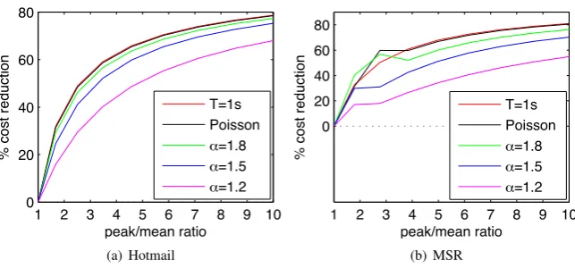
Figure 7: Impact of peak-to-mean ratio on the cost savings of the optimal dynamic resizing.
which shows the cost savings of the optimal dynamic provisioning as compared to the optimal static provisioning for varyingαandT as a function of the switching costβ.
The impact of burstiness on LCP:Interestingly, though Figure 5 shows that the potential of dynamic resizing is limited by increased burstiness, it turns out that the relative performance of LCP is not hurt by burstiness. This is illustrated in Figure 6, which shows the percent of the optimal cost savings that LCP achieves. Importantly, it is nearly perfectly flat as the burstiness is varied.
The Role of the Peak-to-Mean Ratio
The impact of the mean ratio on the potential benefits of dynamic resizing is quite intuitive: if the peak-to-mean ratio is high, then there is more opportunity to benefit from dynamically changing capacity. Figure 7 illustrates this well-known effect. The workload for the figure is generated from the traces by scalingλkas ˆλk=c(λk)γ, varying
γand adjustingcto keep the mean constant.
In addition to illustrating that a higher peak-to-mean ratio makes dynamic resizing more valuable, Figure 7 also highlights that there is a strong interaction between burstiness and the peak-to-mean ratio, where if there is significant burstiness the benefits that come from a high peak-to-mean ratio may be diminished considerably.
The Role of the SLA
The SLA plays a key role in the provisioning of a data center. Here, we show that the SLA can also have a strong impact on whether dynamic resizing is valuable, and that this impact depends on the workload. Recall that in our model the SLA consists of a violation probability ¯εand a delay bound ¯D. We deal with each of these in turn.
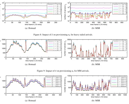
Figures 8 and 9 highlight the role the violation probability ¯εhas on the provisioning ofnkunder the optimal
dy-namic resizing in the cases of heavy-tailed and MM arrivals. Interestingly, we see that there is a significant difference in the impact of ¯εdepending on the arrival process. As ¯εgets smaller in the heavy-tailed case the provisioning gets significantly flatter, until there is almost no change innkover time. In contrast, no such behavior occurs in the MM
case and, in fact, the impact of ¯εis quite small. This difference is a fundamental effect of the “heaviness” of the tail of the arrivals, i.e., a heavy tail requires significantly more capacity in order to counter a drop in ¯ε.
This contrast between heavy- and light-tailed arrivals is also evident in Figure 11, which highlights the cost savings from dynamic resizing in each case as a function of ¯ε. Interestingly, the cost savings under light-tailed arrivals is largely independent of ¯ε, while under heavy-tailed arrivals the cost savings is monotonically increasing with ¯ε.
The second component of the SLA is the delay bound ¯D. The impact of ¯Don provisioning is much less dramatic. We show an example in the case of heavy-tailed arrivals in Figure 10. Not surprisingly, the provisioning increases as ¯D
0 50 100 150 200 250 300 350
102
103
104
105
time frame k (10 mins)
number of servers n
k ε¯= 10−6
¯
ε= 10−5
¯
ε= 10−4
¯
ε= 10−3
¯
ε= 10−2
¯
ε= 10−1
(a) Hotmail
0 100 200 300 400 500 600 700 800 900 101
102 103 104 105
time frame k (10 mins)
number of servers n
k ¯ε= 10−6
¯
ε= 10−5
¯
ε= 10−4
¯
ε= 10−3
¯
ε= 10−2
¯
ε= 10−1
[image:15.595.75.530.108.474.2](b) MSR
Figure 8: Impact of ¯εon provisioningnkfor heavy tailed arrivals.
0 50 100 150 200 250 300 350
0 500 1000 1500 2000
time frame k (10 mins)
number of servers n
k ε¯= 10−6
¯
ε= 10−5
¯
ε= 10−4
¯
ε= 10−3
¯
ε= 10−2
¯
ε= 10−1
(a) Hotmail
0 100 200 300 400 500 600 700 800 900 0
500 1000 1500 2000
time frame k (10 mins)
number of servers n
k ¯ε= 10−6
¯
ε= 10−5
¯
ε= 10−4
¯
ε= 10−3
¯
ε= 10−2
¯
ε= 10−1
(b) MSR
Figure 9: Impact of ¯εon provisioningnkfor MM arrivals.
0 50 100 150 200 250 300 350 400 0
500 1000
time frame k (10 mins)
number of servers n
k D¯= 100ms
¯
D= 200ms
¯
D= 300ms
¯
D= 400ms
¯
D= 500ms
¯
D= 600ms
(a) Hotmail
0 100 200 300 400 500 600 700 800 900 1000
0 500 1000 1500
time frame k (10 mins)
number of servers n
k D¯= 100ms
¯
D= 200ms
¯
D= 300ms
¯
D= 400ms
¯
D= 500ms
¯
D= 600ms
[image:15.595.70.526.115.213.2](b) MSR
Figure 10: Impact of ¯Don provisioningnkfor heavy tailed arrivals.
When is Dynamic Resizing Valuable?
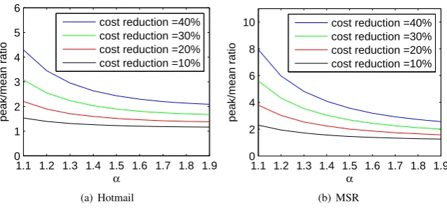
Now, we are finally ready to address the question of when (i.e., for what workloads) is dynamic resizing valuable. To address this question, we must look at the interaction between the peak-to-mean ratio and the burstiness. Our goal is to provide a concrete understanding of for which (peak-to-mean, burstiness, SLA) settings the potential savings from dynamic resizing is large enough to warrant implementation. Figures 12–14 focus on this question. Our hope is that these figures highlight that a precursor to any debate about the value of dynamic resizing must be a joint understanding of the expected workload characteristics and the desired SLA, since for any fixed choices of two of these parameters (peak-to-mean, burstiness, SLA), the third can be chosen so that dynamic resizing does or does not provide significant cost savings for the data center.
10−5 10−4 10−3 10−2 10−1 0
10 20 30
¯ ε
% cost reduction
T=1 Poisson
α=1.8
α=1.5
α=1.2
(a) Hotmail
10−5 10−4 10−3 10−2 10−1 0
20 40 60
¯ ε
% cost reduction
T=1 Poisson
α=1.8
α=1.5
α=1.2
[image:16.595.138.459.115.263.2](b) MSR
Figure 11: Impact of ¯εon the cost savings of dynamic resizing.
1.1 1.2 1.3 1.4 1.5 1.6 1.7 1.8 1.9 0
1 2 3 4 5 6
α
peak/mean ratio
cost reduction =40% cost reduction =30% cost reduction =20% cost reduction =10%
(a) Hotmail
1.1 1.2 1.3 1.4 1.5 1.6 1.7 1.8 1.9 0
2 4 6 8 10
α
peak/mean ratio
cost reduction =40% cost reduction =30% cost reduction =20% cost reduction =10%
(b) MSR
Figure 12: Characterization of burstiness and peak-to-mean ratio necessary for dynamic resizing to achieve different levels of cost reduction.
estimate, one might expectαto be around 1.4-1.6.
Of course, many of the settings of the data center will effect the conclusions illustrated in Figure 12. Two of the most important factors to understand the effects of are the switching cost,β, and the SLA, particularly ¯ε.
Figure 13 highlights the impact of the magnitude of the switching costs on the value of dynamic resizing. The curves represent the threshold on peak-to-mean ratio and burstiness necessary to obtain 20% cost savings from dy-namic resizing. As the switching costs increase, the workload must have a larger peak-to-mean ratio and/or less burstiness in order for dynamic resizing to be valuable. This is not unexpected. However, what is perhaps surprising is the small impact played by the switching cost. The class of workloads where dynamic resizing is valuable only shrinks slightly as the switching cost is varied from on the order of the cost of running a server for 10 minutes (β=1) to running a server for 3 hours (β=18).
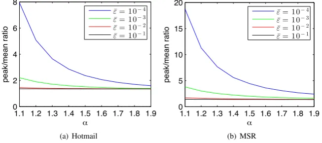
Interestingly, while the impact of the switching costs on the value of dynamic resizing is small, the impact of the SLA is quite large. In particular, the violation probability ¯εcan dramatically affect whether dynamic resizing is valuable or not. This is shown in Figure 14, on which the curves represent the threshold on peak-to-mean ratio and burstiness necessary to obtain 20% cost savings from dynamic resizing. We see that, as the violation probability is allowed to be larger, the impact of the peak-to-mean ratio on the potential of savings from dynamic resizing disappears; and the value of dynamic resizing starts to depend almost entirely on the burstiness of the arrival process. The reason for this can be observed in Figure 8, which highlights that the optimal provisioning nk becomes nearly flat as ¯ε
[image:16.595.138.458.308.457.2]1.1 1.2 1.3 1.4 1.5 1.6 1.7 1.8 1.9 0
2 4 6 8 10
α
peak/mean ratio
β=72
β=18
β=6
β=1
(a) Hotmail
1.1 1.2 1.3 1.4 1.5 1.6 1.7 1.8 1.9 0
1 2 3 4 5 6 7
α
peak/mean ratio
β=72
β=18
β=6
β=1
[image:17.595.135.459.113.263.2](b) MSR
Figure 13: Characterization of burstiness and peak-to-mean ratio necessary for dynamic resizing to achieve 20% cost reduction as a function of the switching cost,β.
1.1 1.2 1.3 1.4 1.5 1.6 1.7 1.8 1.9 0
2 4 6 8
peak/mean ratio
¯ ε= 10−4 ¯ ε= 10−3 ¯ ε= 10−2 ¯ ε= 10−1
(a) Hotmail
1.1 1.2 1.3 1.4 1.5 1.6 1.7 1.8 1.9 0
5 10 15 20
peak/mean ratio
¯ ε= 10−4 ¯ ε= 10−3 ¯ ε= 10−2 ¯ ε= 10−1
(b) MSR
Figure 14: Characterization of burstiness and peak-to-mean ratio necessary for dynamic resizing to achieve 20% cost reduction as a function of the SLA, ¯ε.
Supporting Analytic Results
To this point we have focused on numerical simulations, and further we provide analytic support for the behavior we observed in the experiments above. In particular, the following two theorems characterize the impact of burstiness and the SLA ( ¯D,ε¯) on the value of dynamic resizing under Poisson and heavy-tailed arrivals. This is accomplished by deriving the effect of these parameters onC( ¯D,ε¯), which constrains the optimal provisioningnk. A smaller (larger) C( ¯D,ε¯) implies a smaller (larger) provisioningnk, which in turn implies smaller (larger) costs.
We start providing a result for the case of Poisson arrivals. The proof is given in Section 5.
Theorem 1. The service capacity constraint from Eq. (11) increases as the delay constraintD or the violation prob-¯ abilityε¯decrease. It also satisfies the scaling law
C( ¯D,ε¯)= Θ D¯
−1log ¯ε−1 log ( ¯D−1log ¯ε−1)
!
,
asD¯−1log ¯ε−1→ ∞.
[image:17.595.135.462.321.466.2]the most interesting point about this theorem, however, is the contrast of the growth rate with that in the case of heavy-tailed arrivals, which is summarized in the following theorem. The proof is given in Section 5.
Theorem 2. The implicit solution for the capacity constraint from Eq. (18) increases as the delay constraintD or the¯ violation probabilityε¯decrease, or the value ofαdecreases. It also satisfies the scaling law
C( ¯D,ε¯)= Θ
1
¯
εD¯α−1 !1α
(19)
asε¯D¯α−1→0for any givenα∈(1,2).
A key observation about this theorem is that the growth rate ofC( ¯D,ε¯) with ¯εis much faster than in the case of the Poisson (polynomial instead of logarithmic). This supports what is observed in Figure 11. Additionally, Theorem 2 highlights the impact of burstiness,α, and shows that the behavior we have seen in our experiments holds more generally.
5. Proofs
In this section, we collect the proofs for the results in previous sections. We start with the proof of Lemma 1, the aggregation property used to model the multiserver system with a single service process.
Proof 1 (Proof of Lemma 1). Fix t ≥ 1. Because each server i has a constant rate capacityµ, it follows that the bivariate processes Si(s,t)=µ(t−s)are service processes for the individual servers (see [31], pp. 167), i.e.,
Ri(t) ≥ inf
0≤s≤t{Ai(s)+µ(t−s)}
= 1
n0inf≤s≤t
{A(s)+nµ(t−s)} ,
where Ri(t)is the departure process from server i. In the last line we used the load-balancing dispatching assumption, i.e., Ai(s)= 1nA(s). Adding the terms for i=1, . . . ,n it immediately follows that
P
iRi(t)≥inf0≤s≤t{A(s)+nµ(t−s)},
which shows that the bivariate process S(s,t) = nµ(t−s)is a service process for the virtual system with arrival process A(t)=P
iAi(t)and departure process R(t)=PiRi(t).
We next prove the monotonicity and scaling results in Theorems 1 and 2.
Proof 2 (Proof of Theorem 1). First, note that the monotonicity properties follow immediately from the fact that the function f(x) = (1+x)1x is non-decreasing. Next, to prove the more detailed scaling laws, simply notice that log (1+c f(n))= Θ logf(n)for some non-decreasing function f(n)and a constant c>0. The result follows.
Proof 3 (Proof of Theorem 2). We first consider the monotonicity properties and then the scaling law.
Monotonicity properties: To prove the monotonicity results on D and¯ ε¯, observe that the left hand side (LHS) in the implicit equation from Eq. (18) is a non-increasing function in C( ¯D,ε¯) because the range of the infimum expands whereas the function in the infimum decreases, by increasing C( ¯D,ε¯). Moreover, the LHS is unbounded at the boundary C( ¯D,ε¯)=λ. The solution C( ¯D,ε¯)is thus non-increasing in bothD and¯ ε¯.
Next, to prove monotonicity inα, fixα1≤α2and denote by C1the implicit solution of Eq. (18) forα=α1. In the
first step we prove that C1D¯ ≥1. Let C be the solution of
1
Cα1 =ε¯D¯
α1−1,
where the LHS was obtained by relaxing the LHS of Eq. (18) (we used thatγ >1, C−γλ <C, and x ≥logx for all x≥1). Consequently, C1 ≥C, and by assuming that the units are properly scaled such thatD¯ ≥1, it follows that
Secondly, we prove thatγ, i.e., the optimal value in the solution of C1, satisfiesγ < e. Consider the function
f(γ)= aγloga+1γ with a= α−α1. If, by contradiction,γ≥e, then f0(γ)>0and consequently f(γ)is increasing on[e,∞).
Since the functionC 1
1−γλis also increasing inγ, we get a contradiction thatγis the optimal solution as assumed, and
henceγ <e.
Finally, consider the function g(a)= alogγaγ with a= αα−1. The previous propertyγ <e implies that g0(a)≤0and further that g is non-increasing in a and hence inαas well. Since(C 1
1D¯)α−1 is also non-increasing inα, we obtain that
inf 1<γ<C1
λ γ
(C1D)α1−1(C1−γλ)
γα1−1 α1
logγ α1−1
α1 ≥ inf
1<γ<C1 λ γ
(C1D)α2−1(C1−γλ)
γα2−1 α2
logγ α2−1
α2 .
Using the monotonicity in C1in the term inside the infimum, it follows that C1≥C2, where C2is the implicit solution
of Eq. (18) forα=α1. Therefore, C( ¯D,ε¯)is non-increasing inα.
Scaling law:To prove the scaling law, denote by C the implicit solution of the equation
inf 1<γ<maxC
λ,e 2α α−1 1 Cα γα−1 α
logγα−1α
=ε¯D¯α−1. (20)
The LHS here was constructed by relaxing the function inside the infimum in the LHS of Eq. (18) and extending the range of the infimum. This means that the implicit solution C is smaller than the implicit solution C( ¯D,ε¯). The function inside the infimum of the LHS of Eq. (20) is convex on the domain ofγand attains its infimum atγ=eα−1α . Solving for
C and using that C( ¯D,ε¯)≥C proves the lower bound.
To prove the upper bound, let us fixα,D¯0 andε¯0, and denote by C0( ¯D0, ε0)the corresponding implicit solution.
Using the monotonicity of the implicit solution inε¯D¯α−1, as shown above, it follows that
C( ¯D,ε¯)≥C0( ¯D0,ε¯0),
whereε¯D¯α−1≤ε¯
0D¯α0−1. Fixingγ0=
C0( ¯D0,¯ε0)+λ
2λ , let C be the solution of the equation
γ0
Cα−1(C−γ 0λ)
γα−1α 0
logγ α−1
α 0
=ε¯D¯α−1. (21)
Because the range ofγin the solution of C( ¯D,ε¯)includesγ0, it follows that C( ¯D,ε¯)≤C. On the other hand, the LHS
of Eq. (21) satisfies
γ0
Cα−1(C−γ 0λ)
γα−1α 0
logγ α−1
α 0
≤ K0
Cα , (22)
where K0= γ0
C0( ¯D0,¯ε0)
C0( ¯D0,¯ε0)−γ0λ γα−α1
0
logγα−1α 0
. Here we used that C ≥C0( ¯D0,ε¯0)(note that we showed before that C≥C( ¯D,ε¯)and
C( ¯D,ε¯)≥C0( ¯D0,ε¯0)). Finally, combining Eqs. (21) and (22) we immediately get the scaling law C =O
1 ¯ εD¯α−1
1α
,
and since C( ¯D,ε¯)≤C, the proof is complete.
6. Conclusion
involved in dynamic resizing which we have ignored in this paper. These are all important issues when trying torealize the potentialof dynamic resizing. But, the point we have made in this paper is that whenquantifying the potentialof dynamic resizing it is of primary importance to understand the joint impact of workload and SLA characteristics.
To make this point, we have presented a new model that, for the first time, captures the impact of SLA charac-teristics in addition to both slow time-scale non-stationarities in the workload and fast time-scale burstiness in the workload. This model allows us to provide the first study of dynamic resizing that captures both the stochastic bursti-ness and diurnal non-stationarities of real workloads. Within this model, we have provided both trace-based numerical case studies and analytical results. Perhaps most tellingly, our results highlight that even when two of SLA, peak-to-mean ratio, and burstiness are fixed, the other one can be chosen to ensure that there either are or are not significant savings possible via dynamic resizing. Figures 12-14 illustrate how dependent the potential of dynamic resizing is on these three parameters. These figures highlight that a precursor to any debate about the value of dynamic resizing must be an understanding of the workload characteristics expected and the SLA desired. Then, one can begin to discuss whether this potential is obtainable.
Future work on this topic includes providing a more detailed study of how other important factors affect the potential of dynamic resizing, e.g., storage issues, reliability issues, and the availability of renewable energy. Note that provisioning capacity to take advantage of renewable energy when it is available is an important benefit of dynamic resizing that we have not considered at all in the current paper.
Acknowledgment
This research is supported by the NSF grant of China (No. 61303058), the Strategic Priority Research Program of the Chinese Academy of Sciences (No. XDA06010600), the 973 Program of China (No. 2010CB328105), and NSF grant CNS 0846025 and DoE grant DE-EE0002890.
References
[1] K. Wang, M. Lin, F. Ciucu, A. Wierman, C. Lin, Characterizing the impact of the workload on the value of dynamic resizing in data centers, in: Proc. of the 12th ACM SIGMETRICS/PERFORMANCE joint international conference on Measurement and Modeling of Computer Systems, 2012.
[2] K. Wang, M. Lin, F. Ciucu, A. Wierman, C. Lin, Characterizing the impact of the workload on the value of dynamic resizing in data centers, in: Proc. of the 32th IEEE International Conference on Computer Communications (Infocom mini-conference), 2012.
[3] D. Meisner, B. T. Gol, T. F. Wenisch, PowerNap: Eliminating server idle power, in: ACM SIGPLAN Notices, Vol. 44, 2009, pp. 205–216. [4] L. A. Barroso, U. H¨olzle, The case for energy- proportional computing, Computer 40 (12) (2007) 33–37.
[5] E. V. Carrera, E. Pinheiro, R. Bianchini, Conserving disk energy in network servers, in: Proc. of the 17th annual International Conference on Supercomputing, ICS ’03, ACM, New York, NY, USA, 2003, pp. 86–97.
[6] B. Diniz, D. Guedes, W. Meira, Jr., R. Bianchini, Limiting the power consumption of main memory, in: Proc. of the 34th annual International Symposium on Computer Architecture (ISCA), ACM, New York, NY, USA, 2007, pp. 290–301.
[7] S. Govindan, J. Choi, B. Urgaonkar, A. Sivasubramaniam, A. Baldini, Statistical profiling-based techniques for effective power provisioning in data centers, in: Proc. of the 4th ACM European conference on Computer systems (EuroSys), 2009.
[8] S. Albers, Energy-efficient algorithms, Communications of the ACM 53 (5) (2010) 86–96.
[9] G. Chen, W. He, J. Liu, S. Nath, L. Rigas, L. Xiao, F. Zhao, Energy-aware server provisioning and load dispatching for connection-intensive internet services, in: Proc. of the 5th USENIX Symposium on Networked Systems Design & Implementation (NSDI), 2008.
[10] J. S. Chase, D. C. Anderson, P. N. Thakar, A. M. Vahdat, R. P. Doyle, Managing energy and server resources in hosting centers, in: Proc. of the eighteenth ACM Symposium on Operating Systems Principles, SOSP’01, ACM, New York, NY, USA, 2001, pp. 103–116.
[11] M. Lin, A. Wierman, L. L. H. Andrew, E. Thereska, Dynamic right-sizing for power-proportional data centers, in: Proc. of the 30th IEEE International Conference on Computer Communications (Infocom), 2011, pp. 1098–1106.
[12] T. Lu, M. Chen, L. L. Andrew, Simple and effective dynamic provisioning for power-proportional data centers, IEEE Transactions on Parallel and Distributed Systems 24 (6) (2013) 1161–1171.
[13] A. Greenberg, J. Hamilton, D. A. Maltz, P. Patel, The cost of a cloud: research problems in data center networks, SIGCOMM Comput. Commun. Rev. 39 (2008) 68–73.
[14] D. Meisner, C. M. Sadler, L. A. Barroso, W.-D. Weber, T. F. Wenisch, Power management of online data-intensive services, in: Proc. of the 38th annual International Symposium on Computer Architecture (ISCA), 2011.
[15] J. Heo, P. Jayachandran, I. Shin, D. Wang, T. Abdelzaher, X. Liu, Optituner: On performance composition and server farm energy minimiza-tion applicaminimiza-tion, IEEE Transacminimiza-tions on Parallel and Distributed Systems 22 (11) (2011) 1871–1878.
[16] Q. Zhang, M. F. Zhani, S. Zhang, Q. Zhu, R. Boutaba, J. L. Hellerstein, Dynamic energy-aware capacity provisioning for cloud computing environments, in: Proc. of the 9th International Conference on Autonomic Computing (ICAC), 2012.
[18] E. Thereska, A. Donnelly, D. Narayanan, Sierra: a power-proportional, distributed storage system, Tech. Rep. MSR-TR-2009-153, Microsoft Research (2009).
[19] H. Amur, J. Cipar, V. Gupta, G. R. Ganger, M. A. Kozuch, K. Schwan, Robust and flexible power-proportional storage, in: the 1st ACM Symposium on Cloud Computing (SoCC), 2010.
[20] P. Bodik, M. P. Armbrust, K. Canini, A. Fox, M. Jordan, D. A. Patterson, A case for adaptive datacenters to conserve energy and improve reliability, Tech. Rep. UCB/EECS-2008-127, University of California at Berkeley (2008).
[21] A. Gandhi, M. Harchol-Balter, M. A. Kozuch, The case for sleep states in servers, in: Proc. of the 4th Workshop on Power-Aware Computing and Systems (HotPower), ACM, New York, NY, USA, 2011, pp. 2:1–2:5.
[22] F. Ahmad, T. N. Vijaykumar, Joint optimization of idle and cooling power in data centers while maintaining response time, in: Proc. of the 15th International Conference on Architectural Support for Programming Languages and Operating Systems, ASPLOS’10, ACM, New York, NY, USA, 2010, pp. 243–256.
[23] A. Gandhi, V. Gupta, M. Harchol-Balter, M. A. Kozuch, Optimality analysis of energy-performance trade-offfor server farm management, Performance Evaluation 67 (11) (2010) 1155–1171.
[24] Y. Chen, D. Gmach, C. Hyser, Z. Wang, C. Bash, C. Hoover, S. Singhal, Integrated management of application performance, power and cooling in data centers, in: Proc. of the 12th IEEE/IFIP Network Operations and Management Symposium (NOMS), 2010.
[25] A. Verma, G. Dasgupta, T. K. Nayak, P. De, R. Kothari, Server workload analysis for power minimization using consolidation, in: Proc. of the 2009 conference on USENIX Annual Technical Conference (USENIX ATC), 2009.
[26] M. Lin, Z. Liu, A. Wierman, L. L. Andrew, Online algorithms for geographical load balancing, in: Proc. of the 3rd International Green Computing Conference (IGCC), 2012.
[27] Z. Liu, Y. Chen, C. Bash, A. Wierman, D. Gmach, Z. Wang, M. Marwah, C. Hyser, Renewable and cooling aware workload management for sustainable data centers, in: Proc. of the Proceedings of the 12th ACM SIGMETRICS/PERFORMANCE joint international conference on Measurement and Modeling of Computer Systems, 2012.
[28] SPEC power data on SPEC website at http://www.spec.org.
[29] D. Kusic, J. O. Kephart, J. E. Hanson, N. Kandasamy, G. Jiang, Power and performance management of virtualized computing environments via lookahead control, in: Proc. of the 5th IEEE International Conference on Autonomic Computing (ICAC), 2008.
[30] M. Lin, A. Wierman, L. L. H. Andrew, E. Thereska, Online dynamic capacity provisioning in data centers, in: Proc. of the 49th Allerton Conference on Communication, Control, and Computing, 2011.
[31] C.-S. Chang, Performance Guarantees in Communication Networks, Springer Verlag, 2000.
[32] K. Wang, M. Lin, F. Ciucu, A. Wierman, C. Lin, Characterizing the impact of the workload on the value of dynamic resizing in data centers, Tech. Rep. ISCAS-2014-GD1, available at http://arxiv.org/abs/1207.6295v2 (2014).
[33] F. Ciucu, Network calculus delay bounds in queueing networks with exact solutions, in: Proc. of the 20th International Teletraffic Congress (ITC), 2007, pp. 495–506.
[34] J. Liebeherr, A. Burchard, F. Ciucu, Delay bounds in communication networks with heavy-tailed and self-similar traffic, IEEE Transactions on Information Theory 58 (2) (2012) 1010 –1024.