http://wrap.warwick.ac.uk
Original citation:
Rizk, Amr, Poloczek, Felix and Ciucu, Florin. (2015) Computable bounds in fork-join
queueing systems. ACM SIGMETRICS Performance Evaluation Review, Volume 43
(Number 1). pp. 335-346.
Permanent WRAP url:
http://wrap.warwick.ac.uk/69864
Copyright and reuse:
The Warwick Research Archive Portal (WRAP) makes this work by researchers of the
University of Warwick available open access under the following conditions. Copyright ©
and all moral rights to the version of the paper presented here belong to the individual
author(s) and/or other copyright owners. To the extent reasonable and practicable the
material made available in WRAP has been checked for eligibility before being made
available.
Copies of full items can be used for personal research or study, educational, or not-for
profit purposes without prior permission or charge. Provided that the authors, title and
full bibliographic details are credited, a hyperlink and/or URL is given for the original
metadata page and the content is not changed in any way.
Publisher’s statement:
"© ACM, 2015. This is the author's version of the work. It is posted here by permission of
ACM for your personal use. Not for redistribution. The definitive version was published in
ACM SIGMETRICS Performance Evaluation Review, Volume 43 (Number 1), 2015
http://dx.doi.org/10.1145/2796314.2745859
"
A note on versions:
The version presented here may differ from the published version or, version of record, if
you wish to cite this item you are advised to consult the publisher’s version. Please see
the ‘permanent WRAP url’ above for details on accessing the published version and note
that access may require a subscription.
Computable Bounds in Fork-Join Queueing Systems
Amr Rizk
University of Warwick
Felix Poloczek
University of Warwick / TU Berlin
Florin Ciucu
University of Warwick
ABSTRACT
In a Fork-Join (FJ) queueing system an upstream fork sta-tion splits incoming jobs intoNtasks to be further processed byN parallel servers, each with its own queue; the response time of one job is determined, at a downstream join station, by the maximum of the corresponding tasks’ response times. This queueing system is useful to the modelling of multi-service systems subject to synchronization constraints, such as MapReduce clusters or multipath routing. Despite their apparent simplicity, FJ systems are hard to analyze.
This paper provides the firstcomputablestochastic bounds on the waiting and response time distributions in FJ sys-tems. We consider four practical scenarios by combining 1a) renewal and 1b) non-renewal arrivals, and 2a) non-blocking and 2b) blocking servers. In the case of non-blocking servers we prove that delays scale asO(logN), a law which is known for first moments under renewal input only. In the case of blocking servers, we prove that the same factor of logN dic-tates the stability region of the system. Simulation results indicate that our bounds are tight, especially at high utiliza-tions, in all four scenarios. A remarkable insight gained from our results is that, at moderate to high utilizations, mul-tipath routing “makes sense” from a queueing perspective for two paths only, i.e., response times drop the most when
N = 2; the technical explanation is that the resequencing (delay) price starts to quickly dominate the tempting gain due to multipath transmissions.
Categories and Subject Descriptors
C.4 [Computer Systems Organization]: Performance of Systems; G.3 [Mathematics of Computing]: Probability and Statistics
Keywords
Fork-Join queue; Performance evaluation; Parallel systems; MapReduce; Multipath
Permission to make digital or hard copies of all or part of this work for personal or classroom use is granted without fee provided that copies are not made or distributed for profit or commercial advantage and that copies bear this notice and the full cita-tion on the first page. Copyrights for components of this work owned by others than ACM must be honored. Abstracting with credit is permitted. To copy otherwise, or re-publish, to post on servers or to redistribute to lists, requires prior specific permission and/or a fee. Request permissions from [email protected].
SIGMETRICS’15,June 15–19, 2015, Portland, OR, USA.
Copyright is held by the owner/author(s). Publication rights licensed to ACM. ACM 978-1-4503-3486-0/15/06 ...$15.00.
http://dx.doi.org/10.1145/2745844.2745859.
1.
INTRODUCTION
The performance analysis of Fork-Join (FJ) systems re-ceived new momentum with the recent wide-scale deploy-ment of large-scale data processing that was enabled through emerging frameworks such as MapReduce [12]. The main idea behind these big data analysis frameworks is an elegant divide and conquer strategy with various degrees of freedom in the implementation. The open-source implementation of MapReduce, known as Hadoop [37], is deployed in numerous production clusters, e.g., Facebook and Yahoo [20].
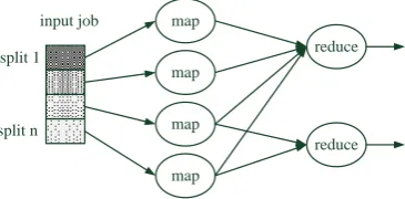
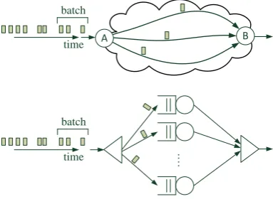
The basic operation of MapReduce is depicted in Figure 1. In themap phase, a job is split into multiple tasks that are mapped to different workers (servers). Once a specific subset of these tasks finish their executions, the corresponding re-duce phasestarts by processing the combined output from all the corresponding tasks. In other words, the reduce phase is subject to a fundamental synchronization constraint on the finishing times of all involved tasks.
A natural way to model one reduce phase operation is by abasic FJ queueing system with N servers. Jobs, i.e., the input unit of work in MapReduce systems, arrive accord-ing to some point process. Each job is split intoN (map) tasks (orsplits, in the MapReduce terminology), which are simultaneously sent to the N servers. At each server, each task requires a random service time, capturing the variable task execution times on different servers in the map phase. A job leaves the FJ system when all of its tasks are served; this constraint corresponds to the specification that the re-duce phase starts no sooner than when all of its map tasks complete their executions.
Concerning the execution of tasks belonging to different jobs on the same server, there are two operational modes. In thenon-blockingmode, the servers are workconserving in the sense that tasks immediately start their executions once the previous tasks finish theirs. In the blocking mode, the mapped tasks of a job simultaneously start their executions, i.e., servers can be idle when their corresponding queues are not empty. The non-blocking execution mode prevails in MapReduce due to its conceivable efficiency, whereas the blocking execution mode is employed when thejobtracker
(the node coordinating and scheduling jobs) waits for all machines to be ready to synchronize the configuration files before mapping a new job; in Hadoop, this can be enforced through the coordination servicezookeeper[37].
map
map
map
map
reduce
reduce input job
split 1
[image:3.595.86.269.55.145.2]split n
Figure 1: Schematic illustration of the basic opera-tion of MapReduce.
The key contribution, to the best of our knowledge, are the first non-asymptotic and computable stochastic bounds on the waiting and response time distributions in the most rel-evant scenario, i.e., non-renewal (Markov modulated) job arrivals and the non-blocking operational mode. Under all scenarios, the bounds are numerically tight especially at high utilizations. This inherent tightness is due to a suitable mar-tingale representation of the underlying queueing system, an approach which was conceived in [23] for the analysis of GI/GI/1 queues, and which was recently extended to ad-dress multi-class queues with non-renewal arrivals [11, 29]. The simplicity of the obtained stochastic bounds enables the derivation of scaling laws, e.g., delays in FJ systems scale as
O(logN) in the number of parallel serversN, for both re-newal and non-rere-newal arrivals, in the non-blocking mode; more severe delay degradations hold in the blocking mode, and, moreover, the stability region depends on the same fun-damental factor of logN.
In addition to the direct applicability to the dimension-ing of MapReduce clusters, there are other relevant types of parallel and distributed systems such as production or supply networks. In particular, by slightly modifying the basic FJ system corresponding to MapReduce, the result-ing model suits the analysis of window-based transmission protocols over multipath routing. By making several sim-plifying assumptions such as ignoring the details of specific protocols (e.g., multipath TCP), we can provide a funda-mental understanding of multipath routing from a queueing perspective. Concretely, we demonstrate that sending a flow of packets over two paths, instead of one, does generally re-duce the steady-state response times. The surprising result is that by sending the flow over more than two paths, the steady-state response times start to increase. The technical explanation for such a rather counterintuitive result is that the logNresequencing price at the destination quickly dom-inates the tempting gain in the queueing waiting time due to multipath transmissions.
The rest of the paper is structured as follows. We first dis-cuss related work on FJ systems and related applications. Then we analyze both non-blocking and blocking FJ sys-tems with renewal input in Section 3, and with non-renewal input in Section 4. In Section 5 we apply the obtained re-sults on the steady-state response time distributions to the analysis of multipath routing from a queueing perspective. Brief conclusions are presented in Section 6.
2.
RELATED WORK
We first review analytical results on FJ systems, and then results related to the two application case studies considered in this paper, i.e., MapReduce and multipath routing.
The significance of the Fork-Join queueing model stems from its natural ability to capture the behavior of many parallel service systems. The performance of FJ queueing systems has been subject of multiple studies such as [4, 26, 35, 21, 24, 5, 7]. In particular, [4] notes that an exact perfor-mance evaluation of general FJ systems is remarkably hard due to the synchronization constraints on the input and out-put streams. More precisely, a major difficulty lies in finding an exact closed form expression for the joint steady-state workload distribution for the FJ queueing system. How-ever, a number of results exist given certain constraints on the FJ system. The authors of [14] provide the station-ary joint workload distribution for a two-server FJ system under Poisson arrivals and independent exponential service times. For the general case of more than two parallel servers there exists a number of works that provide approximations [26, 35, 24, 25] and bounds [4, 5] for certain performance metrics of the FJ system. Given renewal arrivals, [5] sig-nificantly improves the lower bounds from [4] in the case of heterogeneous phase-type servers using a matrix-geometric algorithmic method. The authors of [24] provide an approx-imation of the sojourn time distribution in a renewal driven FJ system consisting of multiple G/M/1 nodes. They show that the approximation error diminishes at extremal utiliza-tions. Refined approximations for the mean sojourn time in two-server FJ systems that take the first two moments of the service time distribution are given in [21]; numerical evidence is further provided on the quality of the approxi-mation for different service time distributions.
The closest related work to ours is [4], which provides com-putable lower and upper bounds on the expected response time in FJ systems under renewal assumptions with Poisson arrivals and exponential service times; the underlying idea is to artificially construct a more tractable system, yet sub-ject to stochastic ordering relative to the original one. Our corresponding first order upper bound recovers theO(logN) asymptotic behavior of the one from [4], and also reported in [26] in the context of an approximation; numerically, our bound is slightly worse than the one from [4] due to our main focus on computing bounds on the whole distribution (first order bounds are secondarily obtained by integration). Moreover, we show that theO(logN) scaling law also holds in the case of Markov modulated arrivals. In a parallel work [22] to ours, the authors adopt a network calculus approach to derive stochastic bounds in a non-blocking FJ system, under a strong assumption on the input; for related con-structions of such arrival models see [18].
asymp-totic results on the response time distribution in the case of renewal arrivals; such results are further used to under-stand the impact of different scheduling models in the reduce phase of MapReduce. Using the model from [32] the work in [33] provides approximations for the number of jobs in a tandem system consisting of a map queue and a reduce queue in the heavy traffic regime. The work in [36] derives approximations of the mean response time in MapReduce systems using a mean value analysis technique and a closed FJ queueing system model from [34].
Concerning multipath routing, the works [3, 17] provided ground for multiple studies on different formulations of the underlying resequencing delay problem, e.g., [16, 38]. Fac-torization methods were used in [3] to analyze the disorder-ing delay and the delay of resequencdisorder-ing algorithms, while the authors of [17] conduct a queueing theoretic analysis of an M/G/∞queue receiving a stream of numbered customers. In [16, 38] the multipath routing model comprises Bernoulli thinning of Poisson arrivals overNparallel queueing stations followed by a resequencing buffer. The work in [16] provides asymptotics on the conditional probability of the resequenc-ing delay conditioned on the end-to-end delay for different service time distributions. ForN = 2 and exponential in-terarrival and service times, [38] derives a large deviations result on the resequencing queue size. Our work differs from these works in that we consider a model of the basic opera-tion of window-based transmission protocols over multipath routing, motivated by the emerging application of multipath TCP [30]. We point out, however, that we do not model the specific operation of any particular multipath transmission protocol. Instead, we analyze a generic multipath trans-mission protocol under simplifying assumptions, in order to provide a theoretical understanding of the overall response times comprised of both queueing and resequencing delays. Relative to the existing literature, our key theoretical con-tribution is to providecomputableand non-asymptotic bounds on thedistributionsof the steady-state waiting and response times under bothrenewal andnon-renewalinput in FJ sys-tems. The consideration of non-renewal input is particularly relevant, given recent observations that job arrivals are sub-ject to temporal correlations in production clusters. For instance, [10, 19] report that job, respectively, flow arrival traces in clusters running MapReduce exhibit various de-grees of burstiness.
3.
FJ SYSTEMS WITH RENEWAL INPUT
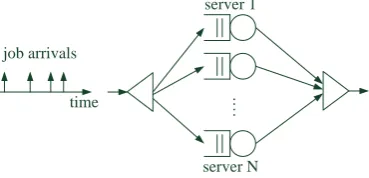
We consider a FJ queueing system as depicted in Figure 2. Jobs arrive at the input queue of the FJ system according to some point process with interarrival timestibetween the
iand i+ 1 jobs. Each jobi is split intoN tasks that are mapped through a bijection toN servers. A task of job i
that is serviced by some servernrequires a random service timexn,i. A job leaves the system when all of its tasks finish their executions, i.e., there is an underlying synchronization constraint on the output of the system. We assume that the families{ti}and{xn,i}are independent.
In the sequel we differentiate between two cases, i.e., a) non-blocking andb) blocking servers. The first case corre-sponds to workconserving servers, i.e., a server starts servic-ing a task of the next job (if available) immediately upon finishing the current task. In the latter case, a server that finishes servicing a task is blocked until the corresponding job leaves the system, i.e., until the last task of the
cur-job arrivals
…
.
time
server 1
[image:4.595.347.532.59.148.2]server N
Figure 2: A schematic Fork-Join queueing system withN parallel servers. An arriving job is split into N tasks, one for each server. A job leaves the FJ system when all of its tasks are served. An arriving job is considered waiting until the service of the last of its tasks starts, i.e., when the previous job departs the system.
rent job completes its execution. This can be regarded as an additional synchronization constraint on the input of the system, i.e., all tasks of a job start receiving service simulta-neously. We will next analyzea) andb) for renewal arrivals.
3.1
Non-Blocking Systems
Consider an arrival flow of jobs with renewal interarrival times ti, and assume that the waiting time of the first job isw1= 0. GivenN parallel servers, thewaiting timewj of thejth job is defined as
wj= max (
0, max
1≤k≤j−1
(
max n∈[1,N]
( k X
i=1
xn,j−i− k X
i=1
tj−i )))
,
(1) for all j ≥ 2, where xn,j is the service time required by the task of job j that is mapped to server n. We count a job as waiting until its last task starts receiving service. Similarly, theresponse timesof jobs, i.e., the times until the last corresponding tasks have finished their executions, are defined asr1= maxnxn,1 for the first job, and forj≥2 as
rj= max
0≤k≤j−1
(
max n∈[1,N]
( k X
i=0
xn,j−i− k X
i=1
tj−i ))
, (2)
where by conventionP0i=1ti= 0; for brevity, we will denote maxn:= maxn∈[1,N].
We assume that the task service timesxn,j are indepen-dent and iindepen-dentically distributed (iid). The stability condi-tion for the FJ queueing system is given asE[x1,1]<E[t1]. By stationarity and reversibility of the iid processes xn,j and tj, there exists a distribution of the steady-state wait-ing time w and steady-state response time r, respectively, which have the representations
w=Dmax
k≥0 (
max n
( k X
i=1
xn,i− k X
i=1
ti ))
(3)
and
r=Dmax
k≥0 (
max n
( k X
i=0
xn,i− k X
i=1
ti ))
, (4)
respectively. Here, =Ddenotes equality in distribution. Note
The following theorem provides stochastic upper bounds onwandr. The corresponding proof will rely on submartin-gale constructions and the Optional Sampling Theorem (see Lemma 6 in the Appendix).
Theorem 1. (Renewals, Non-Blocking) Given a FJ system with N parallel non-blocking servers that is fed by renewal job arrivals with interarrivalstj. If the task service timesxn,jare iid, then the steady-state waiting and response timeswandrare bounded by
P[w≥σ] ≤ N e−θnbσ (5)
P[r≥σ] ≤ NEheθnbx1,1ie−θnbσ , (6)
whereθnb(with the subscript ‘nb’ standing for non-blocking) is the (positive) solution of
E
h
eθx1,1iEhe−θt1i= 1. (7) We remark that the stability condition E[x1,1] < E[t1] guarantees the existence of a positive solution in (7) (see also [29]).
Proof. Consider the waiting timew. We first prove that
for eachn∈[1, N] the process
zn(k) =eθnbPki=1(xn,i−ti)
is a martingale with respect to the filtration
Fk:=σ{xn,m, tm|m≤k, n∈[1, N]} .
The independence assumption ofxn,j andtjimplies that
E[zn(k)| Fk−1] = E h
eθnbPki=1(xn,i−ti) Fk−1
i
= Eheθnb(xn,k−tk)ieθnbPki=1−1(xn,i−ti)
= eθnb
Pk−1
i=1(xn,i−ti)
= zn(k−1), (8)
under the condition on θnb from the theorem. Moreover,
zn(k) is obviously integrable by the condition onθnb from the theorem, completing thus the proof for the martingale property.
Next we prove that the process
z(k) = max
n zn(k) (9)
is a submartingale w.r.t.Fk. Given the martingale property of each of thezn and the monotonicity of the conditional expectation we can write forj∈[1, N]:
Ehmax n zn(k)
Fk−1
i
≥E[zj(k)| Fk−1] =zj(k−1), where the inequality stems from maxnzn(k)≥zj(k) forj∈
[1, N] a.s., whereas the subsequent equality stems from the martingale property (8) forzn(k) for alln∈[1, N]. Hence we can write
E[z(k)| Fk−1]≥max
n zn(k−1) =z(k−1), (10) which proves the submartingale property.
To derive a bound on the steady-state waiting time dis-tribution, letσ >0 and define the stopping time
K:= inf (
k≥0
max n
k X
i=1
(xn,i−ti)≥σ )
, (11)
which is also the first point in time k wherez(k) ≥eθnbσ.
Note that with the representation ofwfrom (3):
{K <∞}={w≥σ}.
Now, using the Optional Sampling Theorem (see Lemma 6 from the Appendix) for submartingales withk≥1:
N = X
n∈[1,N]
EheθnbPki=1(xn,i−ti)i
≥ Ehmax
n e
θnbPki=1(xn,i−ti)i (12)
= E[z(k)]≥E[z(K∧k)]≥E[z(K)1K<k]
≥ eθnbσP[K < k] ,
where we used the condition on θnb from the theorem in the first line, the union bound in the second line, and the submartingale property in the third line. In the last line we used the definition of the stopping timeK; note that we use the notationK∧n:= min{K, n}. The proof completes by lettingk→ ∞.
For the response timer, define the processes
˜
zn(k) =eθnb(Pki=0xn,i−Pki=1ti),
which differs from theznonly in the range of the sum of the service timesxn,i. Then we proceed as for the derivation of the bound on the waiting timew. The only difference in the derivation is that inequality (12) translates to
NEheθnbx1,1i≥Ehmax n e
θnb(Pki=0xn,i−Pki=1ti)i .
Fixing the right hand sides in (5) and (6) to ε, we find that the corresponding quantiles on the waiting and response times grow with the number of parallel serversNasO(logN), a law which was already demonstrated in the special case of Poisson arrival and exponential service times, and for first moments, in [26], and more generally in [4]. This scal-ing result is essential for dimensionscal-ing FJ systems such as MapReduce computing clusters, as it explains the impact of a MapReduce server pool sizeNon the job waiting/response times.
We note that the bound in Theorem 1 can be computed for different arrival and service time distributions as long as the MGF (moment generating function) and Laplace trans-form from (7) are computable. Given a scenario where the job interarrival process and the task size distributions in a MapReduce cluster are not known a priori, estimates of the corresponding MGF and Laplace transforms can be obtained using recorded traces, e.g., using the method from [15].
Next we illustrate two immediate applications of Theo-rem 1.
Example 1: Exponentially distributed interarrival and
service times
Consider that the interarrival timestiand service timesxn,i are exponentially distributed with parameters λandµ, re-spectively; note that when N = 1 the system corresponds to the M/M/1 queue. The corresponding stability condi-tion becomes µ > λ. Using Theorem 1, the bounds on the steady-state waiting and response time distributions are
waiting time
probability
ρ =0.9
ρ =0.75
ρ =0.5
0 25 50 75 100 125 150
10
−6
10
−4
10
−2
10
0
(a) Non-Blocking
waiting time
probability
ρ =0.9
ρ =0.75
ρ =0.5
0 25 50 75 100 125 150
10
−6
10
−4
10
−2
10
0
[image:6.595.108.496.62.209.2](b) Blocking
Figure 3: Bounds on the waiting time distributions vs. simulations (renewal input): (a) the non-blocking case(13)and (b) the blocking case(22). The system parameters areN = 20, µ= 1, and three utilization levels ρ={0.9,0.75,0.5} (from top to bottom). Simulations include100runs, each accounting for107 slots.
and
P[r≥σ]≤N ρe
−(µ−λ)σ
, (14)
where the exponential decay rateµ−λ follows by solving µ
µ−θ λ
λ+θ = 1, i.e., the instantiation of (7).
Next we briefly compare our results to the existing bound on the mean response time from [4], given as
E[r]≤ 1 µ−λ
N X
n=1 1
n . (15)
By integrating the tail of (14) we obtain the following upper bound on the mean response time
E[r]≤log(N/ρ) + 1 µ−λ .
Compared to (15), our bound exhibits the same logN scal-ing law but is numerically slightly looser; asymptotically in
N, the ratio between the two bounds converges to one. A key technical reason for obtaining a looser bound is that we mainly focus on deriving bounds on distributions; through integration, the numerical discrepancies accumulate.
For the numerical illustration of the tightness of the bounds on the waiting time distributions from (13) we refer to Fig-ure 3.(a); the numerical parameters and simulation details are included in the caption.
Example 2: Exponentially distributed interarrival times
and constant service times
We now consider the case of iid exponentially distributed in-terarrival timesti with parameterλ, and deterministic ser-vice timesxn,i= 1/µ, for alli≥0 andn∈[1, N]; note that whenN= 1 the system corresponds to the M/D/1 queue.
The condition on the asymptotic decay rateθnbfrom The-orem 1 becomes
λ λ+θnb
=e−θnbµ ,
which can be numerically solved; upper bounds on the wait-ing and response time distributions follow then immediately from Theorem 1.
3.2
Blocking Systems
Here we consider a blocking FJ queueing system, i.e., the start of each job is synchronized amongst all servers. We maintain the iid assumptions on the interarrival times ti and service timesxn,i. The waiting time and response time for thejth job can then be written as
wj= max (
0, max
1≤k≤j−1
( k X
i=1 max
n xn,j−i− k X
i=1
tj−i ))
rj= max
0≤k≤j−1
( k
X
i=0 max
n xn,j−i− k X
i=1
tj−i )
.
Note that the only difference to (1) and (2) is that the max-imum over the number of servers now occurs inside the sum. It is evident that the blocking system is more conservative than the non-blocking system in the sense that the wait-ing time distribution of the non-blockwait-ing system is domi-nated by the waiting time distribution of the blocking sys-tem. Moreover, the stability region for the blocking system, given by E[t1] > E[maxnxn,1], is included in the stabil-ity region of the corresponding non-blocking system (i.e.,
E[t1]>E[x1,1]).
Analogously to (3), the steady-state waiting and response timeswandrhave now the representations
w=Dmax
k≥0 ( k
X
i=1 max
n xn,i− k X
i=1
ti )
(16)
r=Dmax
k≥0 ( k
X
i=0 max
n xn,i− k X
i=1
ti )
. (17)
The following theorem provides upper bounds onwandr.
Theorem 2. (Renewals, Blocking)Given a FJ queue-ing system withN parallel blocking servers that is fed by re-newal job arrivals with interarrivals tj and iid task service timesxn,j. The distributions of the steady-state waiting and response times are bounded by
P[w≥σ] ≤ e−θbσ (18)
whereθb(with the subscript ‘b’ standing for blocking) is the (positive) solution of
Eheθmaxnxn,1iEhe−θt1i= 1 . (19) Before giving the proof we note that, in general, (19) can be numerically solved. Moreover, for small values ofN,θb can be analytically solved.
Proof. Consider the waiting timew. We proceed simi-larly as in the proof of Theorem 1. LettingFkas above, we first prove that the process
y(k) =eθbPik=1(maxnxn,i−ti)
is a martingale w.r.t. Fk using a technique from [23]. We write
E[y(k)| Fk−1] =E h
eθbPki=1(maxnxn,i−ti) Fk−1
i
=eθbPik=1−1(maxnxn,i−ti)Eheθb(maxnxn,k−tk)i
=eθbPik=1−1(maxnxn,i−ti)
=y(k−1),
where we used the independence and renewal assumptions forxn,i and ti in the second line, and finally the condition onθb from (19).
In the next step we apply the Optional Sampling Theorem (37) to derive the bound from the theorem. We first define the stopping timeKby
K:= inf (
k≥0
k X
i=1
max
n xn,i−ti
≥σ
)
. (20)
Recall thatP[K <∞] =P[w≥σ]. We can next write for everyk∈N
1 =E[y(0)] =E[y(K∧k)]
≥E[y(K∧k)1K<k]
=EheθbPKi=1(maxnxn,i−ti)1K<ki ≥eθbσP[K < k] .
Takingk → ∞completes the proof. The proof for the re-sponse timer is analogous.
Example 3: Exponentially distributed interarrival and
service times
Consider interarrival and service timestiand xn,i that are exponentially distributed with parametersλandµ, respec-tively. In [31] it was shown that
max n Ln=D
N X
n=1
Ln
n
for iid exponentially distributed random variables Ln, so that the stability conditionE[t1]>E[maxnxn,1] becomes
1
λ >
1
µ
N X
n=1 1
n . (21)
By applying Theorem 2, the bounds on the steady-state waiting and response time distributions are
P[w≥σ]≤e−θbσ (22)
and
P[r≥σ]≤ µ µ−θb
e−θbσ ,
whereθbcan be numerically solved from the condition
N Y
n=1
nµ nµ−θb
λ λ+θb
= 1.
For quick numerical illustrations we refer back to Figure 3.(b). The interesting observation is that the stability condition from (21) depends on the number of servers N. In par-ticular, as the right hand side grows in logN, the system becomes unstable (i.e., waiting times are infinite) for suffi-ciently largeN. This shows that the optional blocking mode from Hadoop should be judiciously enabled.
Example 4: Exponentially distributed interarrival and
constant times
If the service times are deterministic, i.e.,xn,i= 1/µfor all
i≥0 andn ∈ [1, N], the representations ofw and r from (16) and (17) match their non-blocking counterparts from (3) and (4) and hence the corresponding stability regions and stochastic bounds are equal to those from Example 2.
4.
FJ SYSTEMS WITH NON-RENEWAL
INPUT
In this section we consider the more realistic case of FJ queueing systems with non-renewal job arrivals. This model is particularly relevant given the empirical evidence that clusters running MapReduce exhibit various degrees of bursti-ness in the input [10, 19]. Moreover, numerous studies have demonstrated the burstiness of Internet traces, which can be regarded in particular as the input to multipath routing.
1 2
p
q
L1 L2
Figure 4: Markov modulating chain ck for the job
interarrival times.
We model the interarrival timestiusing a Markov modu-lated process. Concretely, consider a two-state modulating Markov chainck, as depicted in Figure 4, with a transition matrixT given by
T =
1−p p q 1−q
, (23)
for some values 0 < p, q < 1. In state i ∈ {1,2} the in-terarrival times are given by iid random variables Li with distributionLi. Without loss of generality we assume that
L1is stochastically smaller thanL2, i.e.,
P[L1 ≥t]≤P[L2≥t] ,
for any t ≥ 0. Additionally, we assume that the Markov chaincksatisfies the burstiness condition
number of servers
percentile
ε =10−4
ε =10−3
ε =10−2
0 5 10 15 20
0
10
20
30
40
50
60
(a) Impact ofε
number of servers
percentile
p+q=0.1 p+q=0.9
0 5 10 15 20
0
10
20
30
40
50
60
[image:8.595.110.496.62.209.2](b) Impact of the burstiness factorp+q
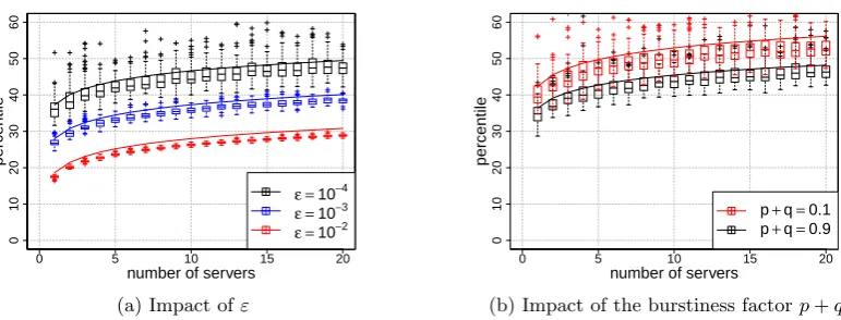
Figure 5: TheO(logN) scaling of waiting time percentileswε for Markov modulated input (the non-blocking case (25)). The system parameters areµ= 1, λ2= 0.9, ρ= 0.75(in both (a) and (b)) p= 0.1, q= 0.4(in (a)),
three violation probabilitiesε (in (a)),ε= 10−4 and only two burstiness parametersp+q (in (b)) (for visual
convenience). Simulations include100runs, each accounting for107 slots.
i.e., the probability of jumping to a different state is less than the probability of staying in the same state.
Subsequent derivations will exploit the following exponen-tial transform of the transition matrixT defined as
Tθ:=
(1−p)E
e−θL1
p E
e−θL2
q E
e−θL1
(1−q)E
e−θL2
,
for someθ >0. Let Λ(θ) denote the maximal positive eigen-value ofTθ, and the vectorh = (h(1), h(2)) denote a cor-responding eigenvector. By the Perron-Frobenius Theorem, Λ(θ) is equal to the spectral radius ofTθ such thathcan be chosen with strictly positive components.
As in the case of renewal arrivals, we will next analyze both non-blocking and blocking FJ systems.
4.1
Non-Blocking Systems
We first analyze a non-blocking FJ system fed with ar-rivals that are modulated by a stationary Markov chain as in Figure 4. We assume that the task service timesxn,j are iid and that the families {ti} and {xn,i} are independent. Note that both the definition ofwjfrom (1) and the repre-sentation of the steady-state waiting timew in (3) remain valid, due to stationarity and reversibility; the same holds for the response times.
The next theorem provides upper bounds on the steady-state waiting and response time distributions in the non-blocking scenario with Markov modulated interarrivals.
Theorem 3. (Non-Renewals, Non-Blocking) Given
a FJ queueing system withN parallel non-blocking servers, Markov modulated job interarrivalstjaccording to the Markov chain depicted in Figure 4 with transition matrix (23), and iid task service timesxn,j. The steady-state waiting and re-sponse time distributions are bounded by
P[w≥σ] ≤ N e−θnbσ (25)
P[r≥σ] ≤ NE
h
eθnbx1,1ie−θnbσ , (26)
whereθnbis the (positive) solution of
Eheθx1,1iΛ(θ) = 1.
(Recall thatΛ(θ)was defined as a spectral radius.)
We remark that the existence of a positive solutionθnbis guaranteed by the Perron-Frobenius Theorem, see, e.g., [29].
Proof. Consider the filtration
Fk:=σ{xn,m, tm, cm|m≤k, n∈[1, N]} ,
that includes information about the stateckof the Markov chain. Now, we construct the processz(k) as
z(k) =h(ck)eθnb(maxnPki=1xn,i−Pki=1ti)
=eθnb(maxnPki=1xn,i−kD) h(ck)eθnb(kD−Pki=1ti)
(27)
with the deterministic parameter
D:=θ−nb1logEheθnbx1,1i .
Note the similarity ofz(k) to (9) except for the additional functionh. Roughly, the functionhcaptures the correlation structure of the non-renewal interarrival time process.
Next we show that both terms of (27) are submartingales. In the first step we note that by the definition ofD:
Eheθnb(Pki=1xn,i−kD)
Fk−1
i
=eθnb(Pik=1−1xn,i−(k−1)D) ,
hence, following the line of argument in (10) the left factor of (27), which accounts for the additional maxn, is a sub-martingale. The second step is similar to the derivations in [9, 13]. First, note that
Ehh(ck)eθnb(D−tk) Fk−1
i
= eθnbDT
θnbh(ck−1)
= eθnbDΛ(θnb)h(c
k−1)
= h(ck−1), (28)
where the last line is due to the definitions of D and θnb. Now, multiplying both sides of (28) byeθnb((k−1)D−Pki=1−1ti)
waiting time
probability
ρ =0.9
ρ =0.75
ρ =0.5
0 25 50 75 100 125 150
10
−6
10
−4
10
−2
10
0
(a) Non-Blocking
waiting time
probability
ρ =0.9
ρ =0.75
ρ =0.5
0 25 50 75 100 125 150
10
−6
10
−4
10
−2
10
0
[image:9.595.108.496.63.209.2](b) Blocking
Figure 6: Bounds on the waiting time distributions vs. simulations (non-renewal input): (a) the non-blocking case (25)and (b) the blocking case (31). The parameters areN = 20, µ= 1, p= 0.1, q = 0.4, λ1 ∈ {0.4,0.72,0.72}
and λ2∈ {0.9,0.9,1.62}leading to utilizations ρ∈ {0.5,0.75,0.9}. Simulations include 100runs, each accounting
for107 slots.
Next we derive a bound on the steady-state waiting time distribution using the Optional Stopping Theorem. Here we use the stopping time K defined in (11). Recall that
P[K <∞] =P[w≥σ]. On the one hand we can write for everyk∈N
E[z(k)] ≥ E[z(K∧k)]
≥ E[z(K∧k)1K<k] = Ehmax
n h(cK)e
θnb(PKi=1xn,i−PKi=1ti)1K<ki
≥ eθnbσE[h(cK)1K<k]
= eθnbσE[h(cK)|K < k]P[K < k] . (29)
On the other hand we can upper bound the term
E[z(k)] =Ehmax
n e
θnb(Pki=1xn,i−kD)i
Ehh(ck)eθnb(kD−Pki=1ti)i ≤NE[h(c1)] .
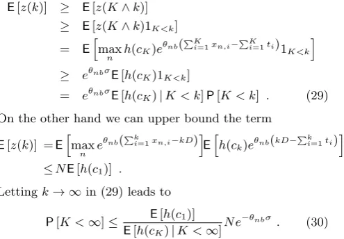
Lettingk→ ∞in (29) leads to
P[K <∞]≤ E[h(c1)]
E[h(cK)|K <∞]
N e−θnbσ . (30)
In Lemma 7 it is shown that the distribution of the ran-dom variable (cK | K < k) is stochastically smaller than the stationary distribution of the Markov chain. Given the burstiness condition in (24) and that the functionhis mono-tonically decreasing [8], we can further upper bound the prefactor in (30) as
E[h(c1)]
E[h(cK)|K <∞]
≤1,
which completes the proof. The proof for the response time
ris analogous.
Remark: Note that, if the burstiness condition (24) is not fulfilled then we can still upper bound the prefactor in (30) using the trivial upper bound
E[h(c1)]
E[h(cK)|K <∞]
≤ E[h(c1)]
minkh(ck) .
Figure 5 displays the bounds on the waiting time per-centiles wε, for various violation probabilitiesε, in the FJ
system with non-renewal input. The bounds closely match the corresponding simulation results, shown as box-plots, while also exhibiting theO(logN) scaling behavior (which can be also derived from both (25) and (26), as in Section 3).
4.2
Blocking Systems
Now we turn to the blocking variant of the FJ system that is fed by the same non-renewal arrivals as in the previous section. Without loss of generality we consider exponential distributionsLm form∈[1,2]. The main result is:
Theorem 4. (Non-Renewals, Blocking)Given a FJ system withN blocking servers, Markov modulated job inter-arrivalstj, and iid task service timesxn,j. The steady-state waiting and response time distributions are bounded by
P[w≥σ] ≤ e−θbσ (31)
P[r≥σ] ≤ Eheθbx1,1ie−θbσ ,
whereθb is the (positive) solution of
Eheθmaxnxn,1iΛ(θ) = 1.
We remark that the positive solution forθbis guaranteed under the stronger stability conditionE[t1]>E[maxnxn,1] and the Perron-Frobenius Theorem.
Proof. LetD :=θ−b1logEeθbmaxnxn,1and define the processyby:
y(k) =h(ck)eθb(Pik=1maxnxn,i−Pki=1ti)
= (eθb(Pki=1maxnxn,i−kD))(h(ck)eθb(kD−Pki=1ti)).
Similarly to the proofs of Theorem 2 and Theorem 3 one can show that both the first and second factor ofyare mar-tingales, and henceyis a martingale. We use the stopping timeKin (20) and write
E[h(c1)] = E[y(0)]
≥ E[y(K∧k)]
≥ E[y(K∧k)1K<k]
= Eheθb(PKi=1maxnxn,i−PKi=1ti)h(c
K)1K<k i
≥ eθbσE[h(c
[image:9.595.56.304.335.507.2]Takingk→ ∞we obtain the bound
P[K <∞]≤ E[h(c1)]
E[h(cK)|K <∞]e
−θbσ ≤e−θbσ ,
where we used Lemma 7 for the last inequality. The proof forris analogous.
A close comparison of the waiting time bound in the non-renewal case (31) to the corresponding bound in the non-renewal case (18) reveals that the decay factors θb depend on sim-ilar conditions, whereby the MGF of the interarrival times in (18) is replaced by the spectral radius of the modulat-ing Markov chain in (31). Moreover, given the ergodicity of the underlying Markov chain, the blocking system with non-renewal input is subject to the same degrading stability region (in logN) as in the renewal case (recall (21)).
For quick numerical illustrations of the tightness of the bounds on the waiting time distributions in both the non-blocking and non-blocking cases we refer to Figure 6.
So far we have contributed stochastic bounds on the steady-state waiting and response time distributions in FJ systems fed with either renewal and non-renewal job arrivals. The key technical insight was that the stochastic bounds in the non-blocking model grow asO(logN) in the number of par-allel servers N under non-renewal arrivals, which extends a known result for renewal arrivals [26, 4]. The same fun-damental factor of logN was shown to drive the stability region in the blocking model. A concrete application follows next.
5.
APPLICATION TO WINDOW-BASED
PROTOCOLS OVER MULTIPATH
ROUTING
In this section we slightly adapt and use the non-blocking FJ queueing system from Section 3.1 to analyze the perfor-mance of agenericwindow-based transmission protocol over multipath routing. While this problem has attracted much interest lately with the emergence of multipath TCP [30], it is subject to a major difficulty due to the likely overtaking of packets on different paths. Consequently, packets have to additionally wait for aresequencing delay, which directly corresponds to the synchronization constraint in FJ systems. We note that the employed FJ non-blocking model is subject to a convenient simplification, i.e., each path is modelled by a single server/queue only.
As depicted in Figure 7, we consider an arrival flow con-taininglbatches ofN packets, withl∈N, at the fork node
A. In practice, a packet as denoted here may represent an entire train of consecutive datagrams. The incoming pack-ets are sent over multiple paths to the destination nodeB, where they need to be eventually reordered. We assume that the batch size corresponds to the transmission window size of the protocol, such that one packet traverses a single path only. For example, the first path transmits the pack-ets{1, N+ 1,2N+ 1, . . .}, i.e., packets are distributed in a round-robin fashion over theN paths. We also assume that packets on each path are delivered in a (locally-)FIFO order, i.e., there is no overtaking on the same path.
In analogy to Section 3.1, we consider a batch waiting until its last packet starts being transmitted. When the transmis-sion of the last packet of batchjbegins, the previous batch has already been received, i.e., all packets of the batchj−1 arein order at nodeB.
…
.
time batch
time batch
[image:10.595.340.532.57.197.2]A B
Figure 7: A schematic description of the window-based transmission over multipath routing; each path is modelled as a single server/queue.
We are interested in the response times of the batches, which are upper bounded by the largest response time of the packets therein. The arrival time of a batch is defined as the latest arrival time of the packets therein, i.e., when the batch is entirely received. Formally, the response time of batchj∈ {lN+ 1|l∈N}can be given by slightly modifying
(2), i.e.,
rj= max
0≤k≤j−1
(
max n
( k X
i=0
xn,j−i− k X
i=1
tn,j−i ))
.
The corresponding steady-state response time has the mod-ified representation
r=Dmax
k≥0 (
max n
( k X
i=0
xn,i− k X
i=1
tn,i ))
.
The modifications account for the fact that the packets of each batch are asynchronously transmitted on the corre-sponding paths (instead, in the basic FJ systems, the tasks of each job are simultaneously mapped). In terms of no-tations, the tn,i’s now denote the interarrival times of the packets transmitted over the same path n, whereas xn,i’s are iid and denote the transmission time of packet i over pathn; as an example, when the arrival flow at node A is Poisson,tn,i has an ErlangEN distribution for allnandi.
We next analyze the performance of the considered mul-tipath routing for both renewal and non-renewal input.
Renewal Arrivals
Consider first the scenario with renewal interarrival times. Similarly to Section 3.1 we bound the distribution of the steady-state response time r using a submartingale in the time domainj∈ {lN+ 1|l∈N}. Following the same steps
as in Theorem 1, the process
zn(k) =eθ(Pki=0xn,i−Pki=1tn,i)
is a martingale under the condition
Eheθx1,1iEhe−θt1,1i= 1, where we used the filtration
Note thatE
e−θt1,1
denotes the Laplace transform of the interarrival times of packets transmitted over each path. The proof that maxnzn(k) is a submartingale follows a sim-ilar argument as in (10). Hence, we can bound the distribu-tion of the steady-state response time as
P[r≥σ] ≤ NEheθx1,1ie−θσ
, (32)
with the condition onθfrom above.
Non-Renewal Arrivals
Next, consider a scenario with non-renewal interarrival times
ti of the packets arriving at the fork node A in Figure 7, as described in Section 4. On every path n ∈ [1, N] the interarrivals are given by a sub-chain (cn,k)k that is driven by theN-step transition matrixTN= (αi,j)i,jforTgiven in (23). Similarly as in the proof of Theorem 3, we will use an exponential transform (TN)θ of the transition matrix that describes each pathn, i.e.,
(TN)θ:=
α1,1β1 α1,2β2
α2,1β1 α2,2β2
,
withαi,j defined above andβ1, β2 being the elements of a vectorβof conditional Laplace transforms ofN consecutive interarrival timesti. The vectorβis given by
β:=
β1
β2
=
Ehe−θPNi=1ti
c1= 1
i
Ehe−θPNi=1ti
c1= 2
i
,
and can be computed given the transition matrix T from (23) via an exponential row transform [9] (Example 7.2.7) denoted by
˜
Tθ:=
(1−p)Ee−θL1 pEe−θL1
qE
e−θL2
(1−q)E
e−θL2
,
yieldingβ= ( ˜Tθ)N
1 1
.
Denote Λ(θ) andh= (h(1), h(2)) as the maximal positive eigenvalue of the matrix (TN)θ and the corresponding right eigenvector, respectively. Mimicking the proof of Theorem 3, one can show for every pathnthat the process
zn(k) =h(cn,k)eθ(Pki=0xn,i−Pki=1tn,i)
is a martingale under the condition on (positive)θ
Eheθx1,1iΛ(θ) = 1. (33) Given the martingale representation of the processeszn(k) for every pathn, the process
z(k) = max n zn(k)
is a submartingale following the line of argument in (10). We can now use (30) and the remark at the end of Section 4.1 to bound the distribution of the steady-state response time
ras
P[r≥σ]≤ E[h(c1,1)] h(2) NE
h
eθx1,1ie−θσ , (34)
where we also used thathis monotonically decreasing and
θas defined in (33).
1 2 3 4 5
0.1
1
10
number of paths
R
~ N
ρ =0.5
ρ =0.75
ρ =0.9
(a) Renewal
1 2 3 4 5
0.1
1
10
number of paths
R
~ N
ρ =0.5
ρ =0.75
ρ =0.9
[image:11.595.326.538.64.201.2](b) Non-renewal
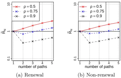
Figure 8: Multipath routing reduces the average batch response time when R˜N <1; smaller R˜N
cor-responds to larger reductions. Baseline parameter µ = 1 and non-renewal parameters: p= 0.1, q = 0.4, λ1={0.39,0.7,0.88}, λ2= 0.95, yielding the utilizations
ρ={0.5,0.75,0.9}(from top to bottom).
As a direct application of the obtained stochastic bounds (i.e., (32) and (34)), consider the problem of optimizing the number of parallel pathsN subject to the batch delay (ac-counting for both queueing and resequencing delays). More concretely, we are interested in the number of pathsN min-imizing the overall average batch delay. Note that the path utilization changes withN as
ρ= λ
N µ ,
since each path only receives N1 of the input. In other words, the packets on each path are delivered much faster with in-creasingN, but they are subject to the additional resequenc-ing delay (which increases as logN as shown in Section 3.1). To visualize the impact of increasing N on the average batch response times we use the ratio
˜
RN:=
E[rN]
E[r1]
,
where, with abuse of notation, E[rN] denotes a bound on the average batch response time for someN, andE[r1] de-notes the corresponding baseline bound for N = 1; both bounds are obtained by integrating either (32) or (34) for the renewal and the non-renewal case, respectively.
In the renewal case, with exponentially distributed inter-arrival times with parameterλ, and homogenous paths/servers where the service times are exponentially distributed with parameterµ, we obtain
˜
RN =
log(N µ/(µ−θ)) + 1 log(1/ρ) + 1
µ−λ θ
, (35)
whereθ is the solution of
µ µ−θ
λ λ+θ
N = 1.
In the non-renewal case we obtain the same expression for ˜
[image:11.595.55.269.411.469.2]RN as in (35) except for the additional prefactor E[h(hc(2)1(1))] prior toN; moreover,θ is the implicit solution from (33).
input; recall that the utilization on each path is Nρ. In both cases, the fundamental observation is that at small utiliza-tions (i.e., roughly when ρ ≤ 0.5), multipath routing in-creases the response times. In turn, at higher utilizations, response times benefit from multipath routing but only for 2 paths. While this result may appear as counterintuitive, the technical explanation (in (a)) is that the waiting time in the underlyingEN/M/1 queue quickly converges to µ1, whereas the resequencing delay grows as logN; in other words, the gain in the queueing delay due to multipath rout-ing is quickly dominated by the resequencrout-ing delay price.
6.
CONCLUSIONS
In this paper we have provided the first computable and non-asymptotic bounds on the waiting and response time distributions in Fork-Join queueing systems. We have ana-lyzed four practical scenarios comprising of either workcon-serving or non-workconworkcon-serving servers, which are fed by ei-ther renewal or non-renewal arrivals. In the case of workcon-serving servers, we have shown that delays scale asO(logN) in the number of parallel serversN, extending a related scal-ing result from renewal to non-renewal input. In turn, in the case of non-workconserving servers, we have shown that the same fundamental factor of logN determines the system’s stability region. Given their inherent tightness, our results can be directly applied to the dimensioning of Fork-Join sys-tems such as MapReduce clusters and multipath routing. A highlight of our study is that multipath routing is reasonable from a queueing perspective for two routing paths only.
Acknowledgement
This work was partially funded by the DFG grant Ci 195/1-1.
7.
REFERENCES
[1] Amazon Elastic Compute Cloud EC2.
http://aws.amazon.com/ec2.
[2] S. Babu. Towards automatic optimization of
MapReduce programs. InProc. of ACM SoCC, pages 137–142, 2010.
[3] F. Baccelli, E. Gelenbe, and B. Plateau. An
end-to-end approach to the resequencing problem.J. ACM, 31(3):474–485, June 1984.
[4] F. Baccelli, A. M. Makowski, and A. Shwartz. The Fork-Join queue and related systems with
synchronization constraints: Stochastic ordering and computable bounds.Adv. in Appl. Probab.,
21(3):629–660, Sept. 1989.
[5] S. Balsamo, L. Donatiello, and N. M. Van Dijk. Bound performance models of heterogeneous parallel
processing systems.IEEE Trans. Parallel Distrib. Syst., 9(10):1041–1056, Oct. 1998.
[6] P. Billingsley.Probability and Measure. Wiley, 3rd edition, 1995.
[7] O. Boxma, G. Koole, and Z. Liu. Queueing-theoretic solution methods for models of parallel and
distributed systems. InProc. of Performance Evaluation of Parallel and Distributed Systems. CWI Tract 105, pages 1–24, 1994.
[8] E. Buffet and N. G. Duffield. Exponential upper bounds via martingales for multiplexers with
Markovian arrivals.J. Appl. Probab., 31(4):1049–1060, Dec. 1994.
[9] C. Chang.Performance Guarantees in Communication Networks. Springer, 2000. [10] Y. Chen, S. Alspaugh, and R. Katz. Interactive
analytical processing in big data systems: A cross-industry study of mapreduce workloads.Proc. VLDB Endow., 5(12):1802–1813, Aug. 2012.
[11] F. Ciucu, F. Poloczek, and J. Schmitt. Sharp per-flow delay bounds for bursty arrivals: The case of FIFO, SP, and EDF scheduling. InProc. of IEEE
INFOCOM, pages 1896–1904, April 2014.
[12] J. Dean and S. Ghemawat. MapReduce: Simplified data processing on large clusters.Commun. ACM, 51(1):107–113, Jan. 2008.
[13] N. Duffield. Exponential bounds for queues with Markovian arrivals.Queueing Syst., 17(3–4):413–430, Sept. 1994.
[14] L. Flatto and S. Hahn. Two parallel queues created by arrivals with two demands I.SIAM J. Appl. Math., 44(5):1041–1053, Oct. 1984.
[15] R. J. Gibbens. Traffic characterisation and effective bandwidths for broadband network traces.J. R. Stat. Soc. Ser. B. Stat. Methodol., 1996.
[16] Y. Han and A. Makowski. Resequencing delays under multipath routing - Asymptotics in a simple queueing model. InProc. of IEEE INFOCOM, pages 1–12, April 2006.
[17] G. Harrus and B. Plateau. Queueing analysis of a reordering issue.IEEE Trans. Softw. Eng., 8(2):113–123, Mar. 1982.
[18] Y. Jiang and Y. Liu.Stochastic Network Calculus. Springer, 2008.
[19] S. Kandula, S. Sengupta, A. Greenberg, P. Patel, and R. Chaiken. The nature of data center traffic: Measurements & analysis. InProc. of ACM IMC, pages 202–208, 2009.
[20] S. Kavulya, J. Tan, R. Gandhi, and P. Narasimhan. An analysis of traces from a production MapReduce cluster. InProc. of IEEE/ACM CCGRID, pages 94–103, May 2010.
[21] B. Kemper and M. Mandjes. Mean sojourn times in two-queue Fork-Join systems: Bounds and
approximations.OR Spectr., 34(3):723–742, July 2012. [22] G. Kesidis, B. Urgaonkar, Y. Shan, S. Kamarava, and
J. Liebeherr. Network calculus for parallel processing. CoRR, abs/1409.0820, 2014.
[23] J. F. C. Kingman. Inequalities in the theory of queues. J. R. Stat. Soc. Ser. B. Stat. Methodol.,
32(1):102–110, 1970.
[24] S.-S. Ko and R. F. Serfozo. Sojourn times in G/M/1 Fork-Join networks.Naval Res. Logist., 55(5):432–443, May 2008.
[25] A. S. Lebrecht and W. J. Knottenbelt. Response time approximations in Fork-Join queues. InProc. of UKPEW, July 2007.
[27] R. Pike, S. Dorward, R. Griesemer, and S. Quinlan. Interpreting the data: Parallel analysis with Sawzall. Sci. Program., 13(4):277–298, Oct. 2005.
[28] I. Polato, R. R´e, A. Goldman, and F. Kon. A
comprehensive view of Hadoop research - a systematic literature review.J. Netw. Comput. Appl., 46(0):1 – 25, Nov. 2014.
[29] F. Poloczek and F. Ciucu. Scheduling analysis with martingales.Perform. Evaluation, 79:56–72, Sept. 2014.
[30] C. Raiciu, S. Barre, C. Pluntke, A. Greenhalgh, D. Wischik, and M. Handley. Improving datacenter performance and robustness with multipath TCP. SIGCOMM Comput. Commun. Rev., 41(4):266–277, Aug. 2011.
[31] A. R´enyi. On the theory of order statistics.Acta Mathematica Academiae Scientiarum Hungarica, 4(3–4):191–231, 1953.
[32] J. Tan, X. Meng, and L. Zhang. Delay tails in
MapReduce scheduling.SIGMETRICS Perform. Eval. Rev., 40(1):5–16, June 2012.
[33] J. Tan, Y. Wang, W. Yu, and L. Zhang.
Non-work-conserving effects in MapReduce: Diffusion limit and criticality.SIGMETRICS Perform. Eval. Rev., 42(1):181–192, June 2014.
[34] E. Varki. Mean value technique for closed Fork-Join networks.SIGMETRICS Perform. Eval. Rev., 27(1):103–112, May 1999.
[35] S. Varma and A. M. Makowski. Interpolation approximations for symmetric Fork-Join queues. Perform. Eval., 20(1–3):245–265, May 1994. [36] E. Vianna, G. Comarela, T. Pontes, J. Almeida,
V. Almeida, K. Wilkinson, H. Kuno, and U. Dayal. Analytical performance models for MapReduce workloads.Int. J. Parallel Prog., 41(4):495–525, Aug. 2013.
[37] T. White.Hadoop: The Definitive Guide. O’Reilly Media, Inc., 1st edition, 2009.
[38] Y. Xia and D. Tse. On the large deviation of
resequencing queue size: 2-M/M/1 case.IEEE Trans. Inf. Theory, 54(9):4107–4118, Sept. 2008.
[39] M. Zaharia, A. Konwinski, A. D. Joseph, R. Katz, and I. Stoica. Improving MapReduce performance in heterogeneous environments. InProc. of USENIX OSDI, pages 29–42, Dec. 2008.
APPENDIX
We assume throughout the paper that all probabilistic ob-jects are defined on a common filtered probability space
Ω,A,(Fn)n,P
. All processes (Xn)n are assumed to be adapted, i.e., for each n ≥ 0, the random variable Xn is
Fn-measurable.
Definition 5. (Martingale) An integrable process(Xn)n is a martingaleif and only if for eachn≥1
E[Xn| Fn−1] =Xn−1 . (36) Further,X is said to be a sub-(super-)martingale if in (36) we have≥(≤) instead of equality.
The key property of (sub, super)-martingales that we use in this paper is described by the following lemma:
Lemma 6. (Optional Sampling Theorem) Let(Xn)n be a martingale, andKa bounded stopping time, i.e.,K≤n
a.s. for somen≥0and{K=k} ∈ Fkfor allk≤n. Then
E[X0] =E[XK] =E[Xn] . (37) IfX is a sub-(super)-martingale, the equality sign in (37) is replaced by ≤(≥).
Proof. See, e.g., [6].
Note that forany(possibly unbounded) stopping timeK, the stopping timeK∧nis always bounded. We use Lemma 6 with the stopping timesK∧nin the proofs of Theorems 1 – 4.
Lemma 7. Letck be the Markov chain from Figure 4 and
K be the stopping time from (11). Then the distribution of (cK|K <∞)is stochastically smaller than the steady-state distribution ofck, i.e.,
P[cK= 2|K <∞]≤P[c1= 2] , or, equivalently,
E[h(cK)|K <∞]≥E[h(ck)] ,
for all monotonically decreasing functionshon{1,2}.
Proof. Using Bayes’ rule and the stationarity of the
pro-cessck, it holds:
P[cK = 2|K <∞] =
∞ X
k=1
P[ck= 2|K=k]P[K=k]
=
∞ X
k=1
P[K=k|ck= 2]P[ck= 2]
=P[c1= 2] ∞ X
k=1
P[K=k|ck= 2] .
Since L1 is stochastically smaller thanL2, we have for any
k≥1
P[K=k|ck= 2]
=P
"
tk≤max n
k X
i=1
xn,i− k−1 X
i=1
ti−σ,max n
k−1 X
i=1
(xn,i−ti)< σ
ck= 2 #
≤P
"
tk≤max n
k X
i=1
xn,i− k−1 X
i=1
ti−σ,max n
k−1 X
i=1
(xn,i−ti)< σ #
=P[K=k] .
Hence P∞