Computing threat points in two player ETP ESP games

(1)

(2)

(3)

Acknowledgements

The first lecture I attended when I started studying was covering statistics and proba-bility. However, being a freshman I entered the wrong lecture hall and ended up at a lecture about economics in health sciences. After I recognized, quite late, that I was sitting at the wrong lecture, I found my way to the correct lecture but had to stand for the remaining hour. I did not know a lot about probability back then, but I did know that the probability of having two of these major mistakes was quite rare. The beginning of the Bachelor was mediocre, but the contrast with the ending of the Master is big.

The last few years within the specialization of Financial Engineering and Manage-ment were unforgettable. First of all I need to thank Reinoud Joosten. Being one of the more eccentric lecturers he was always open for an inspiring discussion within or out-side of the college hours. Not only did he provide me this great subject for graduation, his knowledge in the field of game theory often astonished me. At a certain moment I even recognized that it was also in his interest to have me succeed with this subject, behaviour of a real game theorist. Also I will cherish the discussions about language, dialects, the university, sport and life in general.

Another important person which deserves a special acknowledgement is Berend Roorda. During the specialization Berend was the father of the program. His passion for risk management and finance made a lot of students, including me, enthusiastic about these subjects within the program. During the breaks he was always there to share his knowledge, but was also interested in the well-being of the students. Thank you very much for your hard work and inspiration.

My family also deserves much more credit than they would ever give themselves. Jos, Leontine and Niels, you were always there for me when I needed it the most. Though I know that you had a rougher time with me when I drank a lot of beer and partied too much, I could not have succeeded without your endless support.

Also my friends and loved ones, yes, what to say about you guys. All those times we laughed about the most stupid things and had endless discussions about the most stupid subjects, they provided me with enough distractions to keep focus on the more serious stuff. I would also like to thank all the board members of Integrand and Nesst for providing me an entrepreneurial challenge but also a very steep learning curve outside of the university. And last but not least I want to thank you, the reader, for taking the time to read this thesis.

Rogier Harmelink

(4)

(5)

Abstract

This thesis focuses on the development of algorithms for computing the threat point in Frequency-Dependent-games, with the Endogenous Transition Probabilities (ETP) Endogenous Stage Payoffs (ESP) game as the most complex type of game. We limit ourselves to two-state, two-player ergodic stochastic games with or without a FD payoff. Also incorporated into an algorithm are so-called Endogenous Transition Probabilities, i.e., transition probabilities that depend on the history of the play. Several algorithms have been developed, one of them (SciPy algorithm) only works on non-FD Type I games while the other (Relative Value Iteration algorithm) is limited to use on non-FD Type II games. The Jointly-Convergent Pure-Strategy algorithm works on the broad spectrum of stochastic games described in this thesis, i.e., (non)-FD Type I, Type II and Type III games. We test the algorithms in terms of speed and accuracy and reflect on them including a disquisition of the risks surrounding some of the algorithms. We find that the SciPy algorithm is superior to the Jointly-Convergent Pure-Strategy algorithm in terms of accuracy and speed when computing the threat point in non-FD Type I games. The Relative Value Iteration algorithm works better in terms of accuracy when compared to the Jointly-Convergent Pure-Strategy algorithm but lags in terms of speed. The Jointly-Convergent Pure-Strategy algorithm fits all types of games while finding reasonably accurate solutions in a reasonable time.

(6)

(7)

List of acronyms

AIT Action Independent Transition

CAIT Current Action Independent Transition

CSP Constant Stage Payoffs

CTP Constant Transition Probabilities

ESP Endogenous Stage Payoffs

ETP Endogenous Transition Probabilities

FD Frequency-Dependent

JCPS Jointly-Convergent Pure-Strategy

MDP Markov Decision Process

NaN Not a Number

RVI Relative Value Iteration

(10)

(11)

Chapter 1

Research Design

We start by elucidating the design of our research. We use a well-known method by Verschuren, Doorewaard, and Mellion (2010). Beginning by stating the research objective and the surrounding context. In the second section we derive a framework based on the research objective and context. In order to realize this framework we state research questions (third section) used as a guideline throughout our endeavours. Finally, we conclude by prescribing the structure of this thesis and its aim.

1.1 Research objective and context

Modern game theory is relatively new as a subject in science. Everyone with a little background knowledge in the subject will relate game theory to persons like John Nash Jr. and John von Neumann. The most well-known result in game theory is the Nash equilibrium, but science has evolved and game theory has moved on. Neymann intro-duced a new class in game theory called stochastic games. These stochastic games have been at interest of game theorists all around the globe, but also the subject of new discoveries. One of these discoveries was done in 2003, when Joosten, Bren-ner, and Witt (2003) published research in the field of Frequency-Dependent games.1 Frequency-Dependent games are stochastic games in which the stage payoffs depend on the history of the play. The major theorem in this paper involves so-called ‘threats’. These play an important role in game-theoretical analysis in which they determine the set of possible equilibria. Joosten (2009) stated: “Unfortunately, there exists no general theory on (finding) threat points in FD-games, yet." During the years, more research has been done in the domain of FD-games, e.g. (Mahohoma, 2014), (Joosten, 2015) and (Joosten & Samuel, 2018). Even though the first and last examples focus on com-putations within FD-games, none of these are able to state an exact threat point.

The introduction of Endogenous Transition Probabilities by Joosten and Meijboom (2010) added a novel dimension to the framework of FD-fishery games making analysis

1_{See Section 2.5 for a background on FD-games.}

(12)

of such games more complex. This clearly leaves room for research on the topic of computations of threat points in FD-games. One should see our research as the next step into developing a general theory in finding threat points. We focus on the algorithm building aspect of finding these threat points. Our research objective is to calculate the threat point in ETP-ESP games by developing an algorithm.

1.2 Research framework

In order to complete our research objective we make use of a research framework. In this research framework we describe a few important pillars on which it will rely. The framework can be seen as a stepwise guide being followed in order to complete the research objective. Our research framework is built on the following five pillars.

1. Gather and summarize relevant literature in the game-theoretical domain with a focus on FD-games.

2. Search for and prepare programming tools necessary for the development of the algorithms with a focus on speed.

3. Develop the algorithms.

4. Test the algorithms in terms of speed, accuracy and scalability.

5. Reflect and conclude on the research performed, propose possibilities for future research.

The intended chronological element of our research framework should be clear. We start with a literature study, continue with a search for programming tools which are necessary for the next step: developing the algorithms. At last we test the algorithms and conclude the research in order to give recommendations for later research.

1.3 Research questions

The research framework constructed in the last section serves as a basis for the de-velopment of research questions. The research questions should result in knowledge necessary for achieving the research objective (Verschuren et al., 2010). Each core-question can be answered with the help of so-called sub-core-questions. In this research we only ask one core-question which we define as the main research question. The main research question is also a reflection of the research objective in question form. We state the main research question as:

(13)

1.4. THESIS DESIGN AND AIM 3

We answer this main research question with help of five sub-questions. These are:

1. What has been written in the literature about game theory and Frequency-Dependent games?

2. Which programming tools are available for game-theoretical computations? 3. Which algorithms can find a threat point and how do they work?

4. How do the algorithms perform in terms of speed and accuracy when scaled to a larger game?

5. What can we conclude and recommend based on this research?

As one can see, these sub-questions have a direct link to the research framework. Thus, the answering of the sub-questions should result in completing the steps de-scribed in the research framework which in its part should result in fulfillment of the research objective.

1.4 Thesis design and aim

This chapter describes the research design. In the second chapter we elaborate on all relevant literature surrounding the topic, we start with basic game theory in a gradual fashion ending up at Frequency-Dependent games. Chapter 3 focuses on developing the algorithm, starting with an explanation of the relevant programming tools and later in the chapter the development, testing and practical implications. We conclude and propose recommendations for future research in the fourth chapter.

(14)

(15)

Chapter 2

Game Theory Literature

In the previous chapter we laid a foundation for our research, but in this chapter we start with the necessary background knowledge in the domain of game theory. We start at the origin of game theory and progressively work towards FD-games. In between we discuss important aspects like the Nash equilibrium, repeated games and stochastic games in general. At the end of this chapter a non-expert reader should have the necessary background knowledge in order to follow the steps taken in the development of the algorithm in Chapter 3.

2.1 The Origin of Game Theory

A lot of scientific literature starts with cliché introductions on the complexity of the world we live and breath in. Although it may be a cliché, it is true to a large extent. In order to create structure in the chaos called life, scientists have developed theories and models based on empirical evidence to explain the complexity of life. In social sciences the focus is on explaining behaviour of individuals in a social context. Game theory is a mathematical discipline which forms the (descriptive) basis of analysis of rational decision makers in a strategic environment, in which their decisions have a direct or indirect effect on their individual payoff. According to Hyksova (2004) the first game-theoretical analysis was done by Charles Waldegrave in 1713 as documented in Pierre Rémond de Montmort’s “Essay d’analyse sur les jeux de hazard”, it comprises a strategic solution to the French card game le Her (Bellhouse, 2007).

(16)

We limit ourselves in the remainder to the domain of non-cooperative games, we start with ann players non-cooperative one-shot game in which n = 2. Players play a

game consisting of states, denoted by the state spaceS, a nonempty and finite set. In

a one-shot game players are limited to a game with only1state. Player 1can choose

an action from a nonempty and finite action set Is when in state s ∈ S. Player 2 can

choose an action from a nonempty and finite action setJswhen in states ∈S (Flesch,

1998).

Players can choose an action with probability 1, but they can also randomize by using a mixed action. For player 1 we denote this mixed action by xs in state s ∈ S,

which is a probability distribution onIs. Player2can choose a mixed actionys in state s ∈ S, which is a probability distribution on Js. In a one-shot game with two actions

per player, x ∈ ∆1 ₌ _{_x _∈ _R_|_xi _≥ ₀_for _i _{= 1}_,₂_and P2

i=1xi = 1} and y ∈ ∆1 = {y ∈

R|yi ≥ 0fori = 1,2and P2

i=1yi = 1}. The combination of the (mixed) actions from

both players result in payoffsr1

s1(i1_s1, j_s11)for player1andr2_s1(i1_s1, j_s11)for player2(Flesch, 1998).

Now that we have a mathematical basis we look back at the year 1921. Émile Borel published a few notes from 1921 until 1927 containing the first formalizations of pure and mixed strategies, and even a first attempt at a minimax solution (Borel, 1927). But the real breakthrough in game theory occured when Von Neumann and Morgenstern in 1944 published their work. However this breakthrough was based on earlier work by Von Neumann in 1928, this work already stated the minimax theorem, a revolution in game theory:

Theorem Von Neumann (1928): “For a two-person zero-sum1matrix game (denoted

byM) in which player1 chooses a mixed strategy denoted by pand player 2a mixed

strategy denoted byq. There always exists a pair of mixed strategies(p∗

, q∗) such that."

M(p∗

, q∗

) = max

p minq M(p, q) = minq maxp M(p, q).

(17)

2.1. THEORIGIN OFGAMETHEORY 7

It is best to demonstrate this with an example, consider matrix game zero-sum M

which contains the payoffs for player1as2:

"

7 3 2 2

#

Figure 2.1: Matrix GameM.

Player 1is the row player using strategy p and player2 is the column player using

strategy q. First we look at maxp minq M(p, q). Player 1 wants to maximize his own

payoff and therefore prefers playing the first row over the second one. Given that Player1uses his first action (row), Player2, who wants to minimize the payoff of player 1, will play the right column over the left one because 3 is smaller than 7. The result

of maxp minq M(p, q) = 3. Player 2 who wants to minimize his opponents expected

payoffs uses his second action (column) because this action weakly dominates his first action, meaning that no matter what Player1does, Action2always has a lower payoff

to1than the alternative3. The result of minimax is minq maxp M(p, q) = 3.

2_{We only show the payoffs for player}₁_{as a positive payoff, the payoffs for player}₂_{are the negative} payoff of player1because it is a zero-sum game.

(18)

2.2 The Nash Equilibrium

Where von Neumann can be seen as one of the founding fathers of modern game the-ory, John Nash Jr. (from here on: Nash) can be seen as an absolute rockstar in the world of game theory. In 1951 Nash published his PhD. thesis. A major implication of this thesis was also published in a note called “Equilibrium Points in N-Person Games" (Nash, 1950). Nash won a Nobel Prize in Economics together with John Harsanyi and Reinhard Selten in 1994. He received this prize for the discovery of the solution con-cept for non-cooperative general-sum games. This discovery was later honoured by calling it the Nash equilibrium. Nash stated the following.

Theorem Nash: “Every finite normal form game has at least one equilibrium point

in mixed strategies (Hyksova, 2004)."

Again let’s demonstrate this theorem with the help of two examples. In the first one we demonstrate that in a non zero-sum game there exist two Nash equilibria that are accessible by using a pure strategy for both players. Again player 1 is the row player

with payoff matrixA and player2is the column player with payoff matrix B.

A=

"

9 5 9 3

#

Payoff Matrix Afor Player1.

B =

"

1 5 8 5

#

Payoff MatrixB for Player2.

We combine these matrices to end up with the bimatrix game:

"

9,1 5,5 9,8 3,5

#

Figure 2.2: Bimatrix Game[A, B], first (second) entry is the payoff to player1(2).

In order to check whether a pure Nash equilibrium exists, we set the strategy of one player on a fixed pure strategy and determine the best response of the other player. If a best response of player1is located in the same matrix location as the best response

of player 2 then we can state that the corresponding actions for both players are a

pure Nash equilibrium. Because they are best responses for both players, no player has the incentive to deviate from the Nash equilibrium. Applying this to bimatrix game

[A, B] gives us a new matrix in which we show the best responses of a player with a

(19)

2.2. THENASHEQUILIBRIUM 9

"

9,1 5,5 9,8 3,5

#

Figure 2.3:Bimatrix Game with pure best responses [A, B].

As can be seen in Figure 2.3 the bimatrix game[A, B]has two pure Nash equilibria,

one in which player1plays a pure strategy of playing the bottom row and player 2the

left column. This pure Nash equilbrium is the Pareto optimal result4 _{in this game. The} other equilibrium is when player1plays the upper row with a pure strategy and player 2 the right column with a pure strategy. This equilibrium is a Pareto inferior result in

comparison to the other pure Nash equilibrium.

A pure Nash equilibrium does not have to exist in a bimatrix game, which we show. Again we construct a bimatrix game in which player 1 is the row player with payoffs

in matrixA and player 2 is the column player with payoffs in matrixB, resulting in the

combined bimatrix game[A, B]:

"

3,8 7,5 8,1 6,2

#

Figure 2.4: Bimatrix Game[A, B].

Again we look for the pure best responses, resulting in the following bimatrix:

"

3,8 7,5 8,1 6,2

#

Figure 2.5: Bimatrix Game[A, B].

So Figure 2.5 shows that the bimatrix game [A, B] does not have a pure Nash

equilibrium. However, Nash showed that every bimatrix game in normal form has a mixed Nash equilibrium. For example, player 1 chooses to play the upper row with

probability p and the lower row with probability (1− p). Player 2 on the other side

chooses the left column with probabilityqand the right column with probability (1−q).

The solution for the mixed equilibrium is that player1plays strategy(1 4,

3

4)and player

2strategy(1 6,

5

6). Player1receives a payoff of 6 1

3 and his opponent2 3 4.

(20)

One of the greatest misconceptions surrounding the Nash equilibrium is that it is the optimal outcome for both players in a game. The Nash equilibrium does not have to be the highest possible payoff for an individual player nor for the two players. However, it is the payoff for which each individual player has no rational incentive to unilaterally deviate from. This is demonstrated by the use of the so-called prisoner’s dilemma. In this dilemma two ‘future prisoners’ have the option to cooperate, i.e., not betraying the other player by not telling about the crime, in order to avoid going to prison. The other option is to defect, i.e., selling out the other player by telling. If both players choose to defect, then both go to jail for nine years. If one player defects while the other cooperates, then the player who cooperates is a free man while the other ends up in jail for ten years, if both cooperate they will only serve a one year sentence. This can be shown with the help of bimatrix gameDrepresenting the prisoner’s dilemma.

cooperate def ect

cooperate −1,−1 −10,0 def ect 0,−10 −9,−9

Figure 2.6: Prisoner’s dilemmaD.

(21)

2.3. REPEATEDGAMES 11

2.3 Repeated Games

In the previous section we briefly discussed so-called one-shot zero-sum games and general-sum bimatrix games, i.e., games in which the game is only played once, re-sulting in a single payoff. A repeated game has similarities to the one-shot game. It is a one-shot game but now played for a finite or infinite number of times. The standard assumption is that players are aware of all the (possible) actions and resulting payoffs of the game untilt. We call this complete information (Peters, 2015).

Repeated games have an advantage over one-shot games in the sense that they can reach rewards5 _{which would normally be unattainable (Mertens, 1990). As we} stated earlier, repeated games can be played for a finite or infinite number of times. In the first case this means that the game is played repeatedly for a finite number of times T. The other option is to play the game forever. In game theory the infinitely

repeated type of game is studied more frequently than the finitely repeated game. A reason for this is that it is usually unknown how long T is for a game. Also infinitely

repeated games could be more interesting because finitely repeated games can in specific cases be rewritten as a one-shot game and lack interesting features (Vrieze, 2003b). However, both options result in cumulative payoffs, there are two common methods for the analysis of these cumulative payoffs.

The first common method is the discounted reward criterion, with this criterion we analyze the game by assuming that any future payoff is valued less than the same payoff in the present. Therefore we discount future payoffs with a factor δ(0 < δ <1).

We define the discounted criterion as follows. Playerk receives a discounted reward

(γk_{) in a two player game in which player}₁_{plays strategy}_π_{and player}₂_{plays strategy} σ. The expected payoff of player k at time t under (π, σ) is defined by Rk

t(π, σ). The

discounted reward for player k is:

γk₍_{π, σ}_{) =} T

X

t=0

δt_Rk t(π, σ)

Another way to analyze repeated games is by stating that the player values the present equally to any other period in the future. Therefore the player is indifferent with respect to receiving a payoff now or at a future stage. In this case we are looking at an infinite game with the limiting average reward criterion (Sorin, 2003). For playerk this

is:

γk₍_{π, σ}_{) = lim inf} T→∞ 1 T T X t=1 Rk t(π, σ)

In this thesis we focus on the limiting average criterion. For repeated games the use of this limiting average reward criterion could result in the same rewards as just analyzing a single-period (bi)matrix game.

(22)

2.4 Stochastic Games

We move on to stochastic games. Stochastic games were introducted by Shapley (1953). Stochastic games are much more complex in comparison to repeated games. The only thing in common is that they both are played for a(n) (in)finite number of periods T (T ≥ 2). The difference lies within the state that game is in. In a repeated

game there is only a single state which is played for periodT (T ≥ 2). In a stochastic

game the state can change, based on the transition probabilities of the state in which the game currently is. Such transition probabilities represent the probability of moving to the current state or going to another state. Collectively states can be seen as multiple games that can be played but it depends on the transition probabilities whether they are played or not. Characteristics of one-shot games, repeated games and stochastic games are stated in Table 2.1.

Game type One-shot game Repeated game Stochastic game

T 1 ≥2 ≥2

[image:22.595.104.486.320.375.2]

States 1 1 ≥2

Table 2.1: Characteristics of different types of games.

In order to formalize the stochastic game in general we build further on the frame-work of a non-cooperative game stated in Section 2.1. Again we have n-players (n ≥2), but this time there are a multiple states denoted in the state spaceS. Playeri

hask number of actions depending on the state being in. A strategy is stating exactly

to a player which action to play in each state at each point in time given any history of the play. We usually denote a strategy withπfor player 1andσfor player 2. The

prob-ability of playing a state depends on the transition probabilities, denoted by matrixp. In pthe rows(r)represent the current states while the columns(c)are the possible future

states. An entry inp with row r and column cis the probability of ending up in future

statecfrom current state r. The rows inpshould always sum up to 1 (Pn

c=0pr,c = 1).

The combination of statesS and pair of strategies (π, σ)result together with transition

(23)

2.4. STOCHASTICGAMES 13

In order to make it conceivably we show a simplified example, taken from Samuel’s Master Thesis (2017). The example concerns a two player, two state stochastic game. The payoffs of both players in state1and state2are given byθS₁ andθS₂.

θS₁ =

"

16,16 14,28 28,14 24,24

#

θS₂ =

"

4.0,4.0 3.5,7.0 7.0,3.5 6.0,6.0

#

Ending up in a certain state depends on transition probabilities p, which for both

states are given as:

pS1 ₌

"

0.8,0.2 0.7,0.3 0.7,0.3 0.6,0.4

#

pS2 ₌

"

0.5,0.5 0.4,0.6 0.4,0.6 0.15,0.85

#

This example game is a ‘commons’-type game (Hardin, 1968). In a ‘commons’ game there is a renewable common-pool resource, players share this common-pool and use it for their individual gain which may result in depletion of the resource. A type of game modelled as a ’commons’-type game is the fishery wars, analyzed by Levhari and Mirman (1980) and Joosten (2007). In their fishery wars game the players catch fish from the ocean, but overfishing can result in a depletion of the fish stock. In the example game the depletion of the fish takes place in stateS2, while stateS1represents

a higher amount of fish in the common-pool. Overfishing not only results in a higher probability of ending up in stateS2, but it also affects the transition probabilities. When

overfishing, the transition probabilities change, the transition probability of ending up in stateS2 increases while the probability of ending up in stateS1 decreases.

However, the big question is now, how do we analyze these games? Shapley (1953) proposed using the discounted criterion and proved that there is a value6_{for the infinite} zero-sum game and also showed that minimax and maximin solutions exist. Gillette (1957) introduced the limiting average criterion and showed that a value exists for infi-nite zero-sum games with perfect information. The absolutely compelling proof came from Mertens and Neyman (1981). They showed that a value exists for all zero-sum stochastic games and Neyman (2003a) demonstrated that all stochastic games have a minimax and maximin solution.

6_{The value of a game is the reward of the game when} _M_(p∗_{, q}∗_{) = max}

p minq M(p, q) =

(24)

Types of strategies and Folk Theorem

Finding an equilibrium, a value, a minimax or a maximin solution depends on the type(s) of strategy being chosen by both players. In stochastic games several types of strategies are possible, which we now describe.

Behavioral strategies are strategies in which a player takes into account the history of play leading up to a certain state. Therefore behavioral strategies are history de-pendent and require a player to remember the history of play in order to determine the optimal strategy.

Markov strategiesare strategies in which the player does not take the entire history of play into account, but decides on the basis of the current state the play is in and current period how to play.

Stationary strategiesare strategies in which the decision of the player does not de-pend on the history of play, nor on the current time, it only dede-pends on the current state being in. Therefore a player always plays the same (mixed) action in each state.

Behavioral strategies are the most complex strategy type described here because they require a memory for the player. For infinite stochastic games this requires a large memory, and therefore a lot of storage capacity. However behavioral strategies are not always necessary. In this thesis we limit ourselves to irreducible stochastic games un-der the limiting average criterion. Vrieze (2003a), showed that for irreducible stochastic games stationary strategies are optimal. For reducible stochastic games, the zero-sum game ‘Big Match’ by Blackwell and Ferguson (1968) shows that not all limiting average stochastic games have a value that corresponds to a stationary strategy.

(25)

2.5. FREQUENCY-DEPENDENTGAMES 15

2.5 Frequency-Dependent Games

This brings us to the class of Frequency-Dependent games, introduced in 2003 by Brenner and Witt. Frequency-Dependent games are infinitely repeated games in which the stage payoffs depend on the frequencies of play up until that stage and including the current period in time. The first analysis was done by Brenner & Witt (2003), but Joosten et al. (2003) continued by deepening on feasible results and equilibria.

This was done by introducing the concept of jointly-convergent pure-strategy pairs. An important part of this is the relative frequency vector denoted by xt_{. The relative}

frequency vectorxt _{states the relative frequency of play ending up at a certain payoff}

cumulatively at stage t. As an example we look at a simple 2x2 bimatrix game. The

relative frequency vector at stagetfor this game looks as follows:

xt₌

"

xt

1 xt2

xt

3 xt4

#

Suppose we play this bimatrix game for a period t = 100, the strategy pair (π, σ)

results in the game ending up in x1 for 75 times, in x2 20 times and x4 5 times. The

result is the relative frequency vectorx100 _with:

x100 =

"

0.75 0.20 0.00 0.05

#

For which:

i=4

X

i=1

xi = 1

The relative frequency vector xt _{therefore changes based on frequency of the}

his-tory of play and as stated earlier plays a large role in the concept of jointly-convergent pure-strategy pairs. A pure strategy is a strategy in which at any stage t in any state

a player chooses a certain action with probability 1. A strategy pair (π, σ) is

jointly-convergent for strategy of player 1 π, strategy of player 2 σ and relative frequency

vectorxif and only if (Joosten et al., 2003):

lim sup t→∞

P rπ,σ[|xt

i−xi|> ] = 0

Jointly-convergent pure-strategy pairs are strategy pairs for which the relative fre-quency vector converges to a vector consisting of fixed numbers with probability 1 when t goes to infinity (Billingsley, 2008). Based on this it was possible to compute

(26)

Theorem: “Each pair of individually-rational jointly-convergent pustrategy

re-wards can be supported by an equilibrium. Moreover, each pair of jointly-convergent pure-strategy rewards giving each player strictly more than the threat-point reward, can be supported by a subgame-perfect equilibrium. (Joosten et al., 2003)"

Key in this theorem is the so-called threat point reward. The threat pointv = (v1_{, v}2₎

is defined for two players as the point in which v1 _{= min}

σmaxπγ1(π, σ) and v2 = minπmaxσγ2(π, σ). So both players can threaten each other by minimizing the

pay-off of the other player while the player under threat tries to maximize its own paypay-off. The threat point is the absolute minimum players can reach as a payoff equilibrium and therefore each individual player has an individual rational payoff if he can at least receive the threat point reward (Joosten et al., 2003). But the major result by Joosten et al. (2003) is the following theorem:

Theorem: “Each pair of rewards in the convex hull of all individually-rational

jointly-convergent pure-strategy rewards can be supported by an equilibrium. Moreover, each pair of rewards in the convex hull of all jointly-convergent pure strategy rewards giving each player strictly more than the threat-point reward, can be supported by a subgame-perfect equilibrium (Joosten et al., 2003)."

The threat point is key in finding equilibria supported by jointly-convergent pure-strategy rewards. Threat points can be calculated analytically (e.g.,(Joosten & Meijboom, 2018))7_, but analytical methods may be too cumbersome, and as the complexity of a game in-creases the need for a fast algorithmic solution to compute the threat point inin-creases equally. Joosten and Samuel (2018) have explored the domain of stochastic games and tried to order them. Games are divided into three major categories. Type I, Type II and Type III games. Type I games are games in which the play is repeated and transi-tion probabilities per state are fixed, Type II games are stochastic games with constant transition probabilities and Type III games are stochastic games in which the transition probabilities are endogenous, which means that they depend on the history of play.

(27)

2.5. FREQUENCY-DEPENDENTGAMES 17

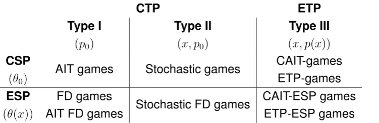
Within these three categories there is also a distinction in whether the payoffs are frequency-dependent. If they are frequency-dependent we call them Endogenous Stage Payoffs (ESP) games. Without the frequency-dependent stage payoffs they are called Constant Stage Payoffs (CSP) games. The same goes for the transition proba-bilities, with frequency-dependent transition probabilities they are called Endogenous Transition Probabilities (ETP) games and Constant Transition Probabilities (CTP) games. Combining these in a table has been done by Joosten and Samuel (2018) and gives the following:

CTP ETP

Type I

(p0)

Type II

(x, p0)

Type III

(x, p(x))

CSP

(θ0)

AIT games Stochastic games CAIT-games

ETP-games

ESP

(θ(x))

FD games

AIT FD games Stochastic FD games

[image:27.595.86.462.233.355.2]

CAIT-ESP games ETP-ESP games

Table 2.2: Ordering of different types of stochastic games (Joosten & Samuel, 2018).

Stochastic Frequency-Dependent (FD) games were first named this way by Mahohoma (2014), Joosten and Samuel (2018) call this term “a tautology in the broad interpreta-tion." Mahohoma (2014) analyzed stochastic FD games while Joosten and Meijboom (2018) analyzed ETP-CSP games. Joosten and Samuel (2018) were the first to calcu-late feasible rewards in ETP-ESP games. In general, the use of the term Frequency-Dependent has been expanding over the years.

The first FD games introduced by Brenner and Witt (2003) and Joosten et al. (2003) were additive. Later, Joosten (2007) introduced an adaptation on the Small Fish Wars which contained FD games that are multiplicative and nonlinear. Joosten (2009) in-troduced the first FD games which are jointly frequency dependent. In 2010, the first FD games with Endogenous Transition Probabilities were developed by Joosten and Meijboom. The last and most complex development in the domain of FD games was tackled by Joosten and Samuel (2018) in the domain of ETP-ESP games.

(28)

(29)

Chapter 3

Building the algorithm

In this chapter we build the algorithm from the ground up, we start by introducing earlier work which partly forms a basis for the algorithm created. Then we clarify the relation between Markov Chains, Markov Decision Processes and Stochastic Games. We in-troduce necessary limitations on stochastic games in order for our algorithm to work as intended. We also introduce the programming tools used to develop the algorithm. Once these things are clear, we start by describing the algorithm(s) for Type I games, then continue with Type II games and end with Type III games. All code corresponding to the algorithms can be found in Appendix A.

3.1 Earlier Work

Before we start with the building blocks of the algorithm, we look at earlier work done in the area of computations in stochastic games. In literature, research has been con-ducted on algorithms for stochastic games. Raghavan and Filar (1991) have concon-ducted a survey in which they limited to algorithms for zero-sum and non-zero-sum stochastic games with complete information and stationary strategies. A lot of research has been done, but mostly regarding the discounted reward criterion (Breton, Filar, Haurle, & Schultz, 1986, e.g.). Vrieze (1981) has developed a linear programming approach to an undiscounted stochastic game based on earlier algorithms by Filar and Raghavan (1979). However it is unclear whether these approaches work on the broad range of stochastic games and if they do, are they able to find the so-called threat point in every type of game?

In 2014 Mahohoma tried to partially overcome this in his Master thesis. He analyzed so-called stochastic FD-games (Type II, CTP-ESP). Part of his thesis is a simulation based approach in MATLAB in order to determine equilibria, feasible rewards but also threat points. However, one of the problems in the approach taken by Mahohoma lies in the simulation approach and the resulting complexity of the code. As an example we

(30)

look at the determination of threat points. Mahohoma simulates the stochastic game for a fixed period t, number of times n. Therefore a total of n simulation results is

combined and gives as an average an approximation of the threat point. Not only does this algorithm lack the ability to give an exact result, the algorithm is also of a high computational complexityO(n4₎_{. This does not mean that the approach of Mahohoma}

is useless, it could be useful in games in which non-stationary strategies are the only way of reaching the threat point. However, when looking at stochastic games in the broader sense, in games in which stationary strategies always cover the threat point, we think that this could be done in an exact and more optimized matter.

The most recent work however has been done by Joosten and Samuel (2018). Samuel (2017) did a first analysis in her thesis. There she started the work which is also partly used for the calculation of threat points in this thesis. Samuel defines three algorithms in MATLAB used for computing feasible rewards in Type I, Type II and Type III games, with or without FD payoff. The basis for the computations of the set of feasible rewards are jointly-convergent pure-strategy rewards in which the algorithm is limited to games with communicating states.1 _{This work has been formalized and} analyzed more rigorously by Joosten and Samuel (2018). The algorithm works well and the threat point is part of the set of feasible rewards found. However, the algorithm does not explicitly find this threat point. Another potential problem with the algorithm is that the computational running time for a large set of rewards possibly is unnecessarily long.

3.2 From Markov Chain to Stochastic Game

In literature there is a clear link between Markov chains on one side, and stochastic games on the other end of the spectrum. Markov chains were introduced by and named after the Russian mathematician Andrey Markov (1971). Markov chains are stochastic processes in which the process is memoryless. The Markov property states that it does not matter what the history is before the present, the only thing relevant for the future is the present. We denote a random variable in a stochastic process at timet by Xt,

the current value of the variable is denoted byx. Mathematically, memorylessness has

the following effect on a stochastic process.

P r(Xt+1 =x|X1 =x1, X2 =x2, . . . , Xt =xt) =P r(Xt+1 =x|Xt =xt) (3.1)

(31)

(32)

Definition Aperiodic Markov Chains: “A Markov chain is said to be aperiodic

if all its states are aperiodic. Otherwise the chain is said to be periodic (Häggström, 2002)."

Figure 3.1 is an aperiodic Markov chain. It is not the case that after a certain fixed number of rainy days that there always will be a sunny day. Aperiodicity and irreducibil-ity are two properties which form the basis of an interesting insight into Markov chains. When an aperiodic and irreducible Markov chain is run for a long time, it is unclear in which state the Markov chain is at a certain period in time. However, running the Markov chain for an infinite period of time will result in the Markov chain settling in a stationary distribution. This stationary distribution describes the probability of visiting a certain state when time goes to infinity. Therefore with great precision we know the frequency of being in a certain state when the Markov chain is run for an infinite period of time. We therefore present an important resulting theorem which forms an important part of this research:

Theorem: “For any irreducible and aperiodic Markov chain, there exists at least

one stationary distribution (Häggström, 2002)."

But how are Markov chains linked to stochastic games? Neymann described that “Markov chains and Markov decision processes are special cases of stochastic games (Neyman, 2003a)." Markov chains are necessary to model the dynamics of a system. They state the transition probabilities of a stochastic game. In between the Markov chain and the stochastic game is the Markov Decision Process (MDP). The MDP is a reduction of the stochastic game in which there is only one player. Therefore the player is able to control the play and hence the corresponding payoffs on his own. Filar and Vrieze (1997) describe the stochastic game in terms of a competitive MDP.

In the case of one player under the limiting average criterion they describe the MDP as follows. The player starts in initial state s while playing stationary strategy f, the

reward at timet is defined byRt. The value of this irreducible limiting average MDP is

defined as (Filar & Vrieze, 1997):

vα(f) := lim T→∞

1 T + 1

T

X

t=0

Esf[Rt]

The individual rational player always wants to maximize his own payoff. So the problem is an optimal control problem in which the player wants to:

(33)

3.3. LIMITATIONS GAME USAGE 23

This problem can also be seen as an optimal control problem in which the player tries to control the process in such a matter that his own value is maximized (Blackwell, 1962). In literature these MDP models are not only used for stochastic games but for a wide range of applications. They are used for decision-theoretic planning, learning robot control and ofcourse stochastic games. MDPs are the standard for learning se-quential decision making (Otterlo, 2009). Algorithms in order to find optimal values for an MDP are divided into two categories. Model-free and model-based algorithms. The first category is also known as reinforcement learning and generates approximations while the second one is exact and uses dynamic programming as a basis (Blackwell, 1962), (Otterlo, 2009).

Because we are dealing with stochastic games in which we assume perfect infor-mation we have all inforinfor-mation available in order to calculate an exact result. We shall therefore only look at model-based algorithms. These algorithms work on optimizing value functions by either iterating over the value function (value iteration) or by chang-ing the so-called policy (policy iteration). The policy of an MDP can be seen as a fixed pure strategy which always is taken when in a certain state. At the heart of these algo-rithms is the Bellman equation. The Bellman equation defines the relation between the value function and the recursive process in order to determine the result of the value function (Otterlo, 2009). The equation is stated as (Otterlo, 2009):

Vπ₍_s_{) =}

Eπ

rt+Vπ₍_st

+1)|st=s

=X

s0

T(s, π(s), s0

) R(s, a, s0

) +Vπ(s0

)

In which policy is represented byπ, the transitions by T, current state bys, rewards

by R and current reward by r. This Bellman equation is important when we come

to an algorithm for Type II games. But for now it is most important to acknowledge that stochastic games can be seen as competitive MDPs in which Markov chains are responsible for the transition dynamics between the states.

3.3 Limitations game usage

(34)

For the general-sum case there exist-equilibria2, but optimal stationary equilbria are

only known to exist in a select number of cases (Flesch, 1998).

We limit ourselves in the creation of the algorithm to types of games for which we know that the algorithm works. Earlier we stated Markov chain properties which guar-antee a stationary distribution of the chain, i.e., irreducibility and aperiodicity. There-fore we focus on games in which the Markov chain governing the transition matrix is ergodic.3 _{Games with absorbing states or more than one ergodic set are currently left} out of scope. This however, does not mean that the algorithm constructed does not cope with any of the special classes described by Flesch (1998). We think that this leaves room for future research. For now we focus on the above stated characteristics and type of games displayed in Figure 2.2. We limit ourselves to two-player, two-state games.

3.4 Programming Tools

Creating an algorithm has to be done with the help of programming languages and tools. Earlier we stated that work has been done by Mahohoma (2014) and Samuel (2017) in MATLAB. We choose to deviate from MATLAB and take a different approach. First, MATLAB is a commercial programming language used mostly in the educational domain, but because of the commercial licensing necessary to run, it limits the appli-cability of the algorithm without a license. We are however in favor of free open-source solutions. Secondly, because MATLAB is a commercial product we cannot always get a grasp on what is happening under the hood of the program. In case of algorithmic optimization this can be problematic. So a choice has been made to not continue us-ing MATLAB but to transfer to Python. We describe Python and the other programmus-ing tools used briefly to give the reader an impression of their possibilities.

3.4.1 Python

We first introduce the main programming language used. Python was developed in the early 90’s by Guido van Rossum. The goal of Python is to provide easy and un-derstandable syntax, which should result in highly readable code. Python does this by using indentation as a major part of the programming syntax. In comparison to other programming languages, Python has a dynamic type system, i.e., that Python does not require the programmer to define the type of variables used. This also improves readability a lot. On the other side, Python is an interpreted language and also a rather slow one. In comparison to C++ or Java, Python lacks raw speed. However, Python

2_{-equilibria are equilibria that approximately satisfy the condition associated with the Nash} equilib-rium. The incentive for a player to deviate from this equilibrium issmall.

(35)

3.5. TYPEIGAMES 25

is a flexible language for which additional packages can be used to cope with this. A lot of additional and highly optimized packages are developed for Python and can be used.

3.4.2 NumPy

One of these packages is NumPy and was introduced in 2005 into Python. NumPy is written in C and offers Python users multi-dimensional array and matrix tools. It is seen as the go to solution for numerical computations with high-level4 _mathematical functions. Because NumPy has been written and compiled in C the operations are comparable to MATLAB in terms of speed. NumPy is also open-source and develop-ment is ongoing, so it is well-suited for the building of the algorithm in this thesis.

3.4.3 SciPy

Another comparable package is SciPy, SciPy is based on NumPy and uses a lot of at-tributes from NumPy in order to provide scientific computing functions. SciPy contains for example linear algebra functions and optimization functions using linear program-ming.

3.4.4 MDP Toolbox

The last tool used is the Python MDP Toolbox. This toolbox contains multiple algorithms (model-free and model-based) which can be used in order to solve an MDP. Most algorithms are written with the help of NumPy and therefore speed should not be an issue.

3.5 Type I games

We start building the algorithm by looking at Type I games. They are simple in essence because the play in these games is repeated. This makes Type I games less hard to analyze in comparison to Type II, let alone Type III games. But first we should state how we enter a game into the algorithm(s). We use NumPy in order to declare matrices. In Type I games, only two things are relevant when entering the game into an algorithm. Most important are the reward matrices for each player, the reward matrices display the payoffs that a player can achieve when playing pure strategies. Next is the frequency-dependent function, the frequency-frequency-dependent function declares what the relation is

(36)

between a potential change in payoff and the frequency of play of certain strategy combinations. Because both can be defined in several ways, we adapt to the model used by Samuel (2017). Samuel (2017) uses a game in which the Nash equilibrium is also Pareto superior. However, she states that when playing this equilibrium this will eventually have an impact on the renewable common-pool resource and will therefore influence the payoff in the future (Samuel, 2017).

The combined payoff matrix used in order to test the algorithm is as follows:

θS₁ =

"

16,16 14,28 28,14 24,24

#

Samuel also created a linearly decreasing function as the frequency-dependent function. This was specifically created for the game stated above, so we also use this function in order to test the algorithm within this thesis.5

The frequency-dependent function for the Type I game is determined by:

F DIt = 1− 1 4(x

t

2+ 2x

t

3)−

2xt

4

3

Hence, if the payoffs are frequency-dependent, they become:

θt

S1 =F D

t I ·

"

16,16 14,28 28,14 24,24

#

The upper-left corner of the payoff matrix (with payoff 16 to both players) can be seen as the responsible result of the game for which the depletion of the common-pool resource is non-existent. The upper-right corner results in a slight depletion, while the bottom-left corner is double the depletion compared to the upper-right corner. The worst outcome for the common-pool resource would be the bottom-right corner, it would result in the largest depletion effect on the renewable common-pool resource. There-fore the players also have to take into account the long-term effect on the common-pool resource.

But now we focus on the building of the algorithm. Because there are different ways to skin a cat, there are also different ways to build an algorithm. We have tested two approaches and will start with the approach which uses a SciPy optimizer. The second approach is an adaptation of the algorithm by Joosten and Samuel (2018).

(37)

3.5. TYPEIGAMES 27

3.5.1 SciPy optimizer

SciPy as stated earlier is home to scientific computing packages. One of these is the optimization package. The optimization package contains several mathematical optimizers which are used for finding local or global optima. Mostly these optimizers rely on methods which calculate derivatives in order to find the optimum of a function. However a problem with these methods is that they can get stuck in local optima which could potentially not be the global optimum (Knowles, Watson, & Corne, 2001). Using these optimizers therefore has an inherent risk, which is that they provide possible sub-optimal solutions.

For Type I games with no frequency-dependent function this problem is redundant. Type I games as stated earlier are simple games which are repeated for a(n) (in)finite number of periods. Therefore optimizing over the payoffs is like optimizing a linear function when searching for a minimum. We start by using the optimizer for non-FD Type I games.

Because we are looking at the threat point for two players we start by restating what the threat point is. The threat pointv is the point in which player1plays strategyπand

player2plays strategyσ for which:

v = (v1, v2) with:

v1 = min σ1 max_π1 γ

1₍_π1_{, σ}1₎

v2 = min π2 max_σ2 γ

2₍_π2_{, σ}2₎

Sov1 (2)_{is the amount which player}₁₍₂₎_{can guarantee himself if player}₂₍₁₎_{tries to}

minimize the payoff of player1(2).

In order to find the threat point we start in Python by initializing the strategy of the player who is threatening the other player with an empty strategy (an array containing only zeros). Then we have to set a condition for which the stationary strategy must hold. This condition declares that the probability assigned to all possible actions within the strategy must sum to 1. For example, if we have a game with one-state and two

possible actions for player 2, if σ1, σ2 are the representation of player 2 choosing

re-spectively action1, action2then

2

X

i=1

σi = 1

So again, the player has to choose a stationary strategy in which there is a summed probability of1over all possible actions. Additionally we have to declare to the algorithm

(38)

0≤σi ≤1

We also declare a threat function, this is the function that needs to be optimized. In this case we first multiply the rewards with the stationary strategy chosen by the threatening player, i.e., forv1we multiplyγ1withσ1. Therefore functionv1has the form:

v1 = max π1 (γ

1_·_σ1₎

And forv2_:

v2 = max σ2 (γ

2_·_π2₎

This threat function is then applied within the optimizer, together with the sum con-straint and the boundary conditions. The optimizer adjusts the strategy for the player under threat in order to receive the maximum reward possible. The optimizer is run based on sequential quadratic programming and finds a solution based on the given input. Summarizing the algorithm works as follows:

Algorithm 1Threat point algorithm Type I non-FD game with SciPy optimizer.

Input: Reward matrix Player1, Player2

Output: Threat pointv = (v1_{, v}2₎

1: Declare that strategies must sum to1

2: Declare that each action has a probability bound between0and1 3:

4: Initialize strategy pairσ1

5: Declare threat functionv1

6: Run SLSQP optimizer with constraints and bounds forv1

7: Print the result ofv1

8:

9: Initialize strategy pairπ2

10: Declare threat functionv2

11: Run SLSQP optimizer with constraints and bounds forv2

12: Print the result ofv2

13:

14: Return threat pointv = (v1_{, v}2₎

Running this algorithm for the example game stated above finds the threat point in 0.005 seconds6_{. The algorithm returns as a threat point} _v _{= (24}_,₂₄₎_{, which is the}

(39)

3.5. TYPEIGAMES 29

correct threat point for this game. We have confirmed this by computing the maximin value of the game, which was23.9. We were not able yet to incorporate the

frequency-dependent function into the SciPy algorithm. We have looked into multiple methods but have not found an efficient and satisfactory solution.

3.5.2 Jointly-Convergent Pure-Strategy Algorithm

As stated earlier, the previous algorithm is one way to find the threat point. We have developed another algorithm based on earlier work by Joosten and Samuel (2018). However, we keep in mind that the implementation of Samuel (2017) could be opti-mized further. This algorithm also contains necessary building blocks for the algo-rithms of Type II and Type III games. Therefore we gradually build the algorithm and state necessary functions for all algorithms (Type I, II and III) in this section.

We start with the first element. Again we want to fix the strategy for the player who is threatening the other player. In this algorithm however, we want to draw random strategies from aβ-distribution. We draw them from theβ-distribution because theβ

-distribution has nice properties. One of these is that when set accordingly (α =β = 0.5)

the β-distribution tends to draw more values at the edges of the distribution (at 0and 1). In these ‘less likely’ values there is a higher chance that there are more interesting

things to occur (Samuel, 2017).

Function wise we built the following function:

Algorithm 2Function: Draw Random Strategy.

Input: Total points to generate, number of total actions for player who threatens

Output: Random strategy matrix

1: Draw points number of strategies with a length of number of total actions from a β-distribution with (α=β = 0.5)

2: Normalize the drawn strategies, such that each individual strategy sums to one

3: Return the random strategy matrix

Samuel used theβ-distribution to draw frequency vectors, but she implemented this

with an unoptimized for-loop making computing time much longer than necessary. In this version we vectorize the code as much as possible in order to improve computing speed. Vectorization delivers a direct improvement in computing speed by reducing complexity of code.

(40)

strategy, we only consider pure stationary strategies for the player who is being threat-ened. Therefore we have to convert the strategy of the player who is threatening into a frequency vector based on the pure stationary strategy reply of the player under threat. Based on this we built a function which sorts strategies into frequency vectors. For each individual player we built a separate function, but this is due to storage differences, in essence they are comparable. The function contains:

Algorithm 3Function: Create Frequency Vector.

Input: Total points generated, number of total actions for both players, random strategy

matrix

Output: Frequency pairs based on pure best replies from player under threat

1: Initialize frequency vector with dimensions: (total number of points·total number of actions Player 1, total number of actions Player 1· total number of actions Player

2)

2: foriin rangetotal number of actions player under threat do

3: forj in rangetotal number of actions threatening player do

4: if v1 _{is searched} _then _{frequency vector[total number of points} _· ₍_i₋₁_):total

number of pointsi,(number of actions player 2·i)+j] = random strategy matrix[:,j]

5: end if

6: if v2 _{is searched} _then _{frequency vector[total number of points} _· ₍_i₋₁_):total

number of pointsi,(number of actions player 1·j)+i] = random strategy matrix[:,j]

7: end if

8: end for

9: end for

10: Return frequency vector

The result is a frequency vector in which only the pure stationary best replies of the player under threat contain a non-zero frequency of play. As an example, if a player under threat has two pure stationary strategies (as an example: left and right) as a reply, then if there are 200 random strategies drawn for the threatening player,

the result is 400 frequency pairs in the frequency vector. The first 200 represent the

first (left) pure stationary strategy of the player under threat, the second200represent

the other (right) pure stationary strategy. We visualize this with an example, suppose the player threatening plays a mixed stationary strategy in which up is played with probability 0.8 and down with probability 0.2. Algorithm 3 then sorts this strategy in

(41)

3.5. TYPEIGAMES 31

"

0.8 0 0.2 0

#

and

"

0 0.8 0 0.2

#

(3.2)

Figure 3.2: Best reply frequency matrices.

There is a trade-off taking place in this frequency vector function. By creating this function it was inevitable to use a for-loop. Because we want to create a function which can scale with larger games with more actions, we had to use a for-loop. However, this for-loop was done with a NumPy for-loop, an optimized way of running a for-loop in large matrices. Performance gains can be made if the number of actions for a game is always fixed at the same number, in those cases a hard-coded function without for-loops will result in a significant gain in computational performance.

At last we need to build a function which stores all the corresponding drawn random mixed strategies with pure best responses into a logical matrix which makes extracting the threat point easy. Therefore we built a function called payoff sort. This function sorts the payoffs which are computed from the generated random mixed strategies based on there relationship. So the function stores all pure best replies to a certain drawn strategy in the same row. Function wise this has resulted in the following:

Algorithm 4Function: Payoff sort.

Input: Total points generated, payoff matrix, total number of actions

Output: Sorted payoff matrix

Initialize empty sorted payoff matrix (number of points, number of actions)

forxin range total number of pointsdo foriin range total number of actionsdo

Sorted payoffs[x,i] = payoff matrix[points·i+x]

end for end for

Return sorted payoff matrix

(42)

Algorithm 5(Non)-FD Type I threat point algorithm.

Input: Type I Game, total number of points, activate FD function

Output: Threat point

1:

2: Ifv1 _{is calculated, then}_X _{= 1}_,_Y _{= 2}_,

3: Ifv2 _{is calculated, then}_X _{= 2}_,_Y _{= 1}

4:

5: Turn reward matrix PlayerX into flattened reward vector 6: Threatening strategies PlayerY = Draw Random Strategies

7: Best response PlayerX frequency vector = Create Frequency Vector 8: ifActivate FD function = Truethen

9: Activate and Calculate FD payoff Function result

10: end if

11: Payoffs PlayerX = Sum over all columns of: (Frequency Vector per row·flattened vector PlayerX)

12: ifFD Function is activethen

13: Element wise multiplication of FD payoff function result with Payoffs PlayerX

14: end if

15: Sorted payoff matrix = Payoff sort

16: Pick the maximum value of each row of the sorted payoff matrix as best response of PlayerX

17: Pick the minimum value over all rows as the result ofvX 18:

19: Return threat pointv = (v1_{, v}2₎

Filling in a total number of points generated of 100 and the FD payoff function as

not active results in a threat point of approximately (24.009,24.0006) in roughly 0.006

seconds. When activating the FD payoff function the algorithm finds a threat point with

100points in roughly the same amount of time with as a result(10.506,8.0002).

3.5.3 Visualizing the results

(43)

(44)

The effect of the depletion of the common-pool resource can clearly be seen in Figure 3.4. In this game in which the FD payoff function is activated the players still play the same payoff in case of the threat point, which is the bottom-right corner of the example game resulting in the depletion of the common-pool resource. The result of this depletion effect is that even the lowest possible pure payoff (16,16) in the

non-FD situation is now a Pareto optimal solution. The players can threaten each other by depleting the common-pool resource and after wards can reach several payoffs denoted by the black lines north-east of the threat point.

3.5.4 Comparing the two algorithms

The question that still is unanswered is: which of the algorithms should we use for Type I games? For Type I FD-games it is quite easy to choose, because the SciPy algorithm does not incorporate FD payoff functions we cannot use this algorithm for Type I FD-games. However, for Type I non-FD-games we have a choice between the SciPy algorithm and the jointly-convergent pure-strategy algorithm. We test both algorithms in terms of running time and decimal accuracy. We construct three games to test:

1. The example game

2. A random game of size 4x4 3. A random game of size 10x10

For both algorithms these games are run, for the jointly-convergent pure-strategy algorithm we enter multiple amounts of points in order to increase accuracy. However, we must state that for the random games we simply do not know the exact threat point, we could compute this by hand, but because this takes a lot of time we trust that the algorithms should be a good approximation. We check this approximation by calculating the maximin result, subtracting the best approximation for the maximin result from the best approximation for the threat point should give us a reasonable indication of the algorithm accuracy. We start by testing both algorithms on the example game.

# points JCPS-Algorithm JCPS Algorithm Result Run-time JCPS SciPy Optimizer Result Run-time SciPy Difference JCPS - SciPy 100 (24.009, 24.0006) 0.006 seconds (24., 24.) 0.005 seconds (0.009, 0.0006)

10,000 (24.00000002, 24.00000037) 0.29 seconds (24., 24.) 0.005 seconds (2 * 10^-8, 3.7 * 10^-7)

1,000,000 (24.000000000004057,

24.000000000000398) 26.34 seconds (24., 24.) 0.005 seconds

(4.057 * 10^-12, 3.98 * 10^-13)

(45)

3.5. TYPEIGAMES 35

As the results show in Table 3.1 the SciPy optimizer finds the exact threat point within 0.005 seconds while the jointly-convergent pure-strategy algorithm can find ap-proximations with 100 points with an accuracy of two decimals. Increasing the number of points generated also increases accuracy a lot, to seven decimals, but also increas-ing the run-time of the algorithm to 0.29 seconds. For 1,000,000 points, the increase in accuracy is much lower compared to the increase time necessary to compute the algorithm. The SciPy algorithm is clearly the winner in this comparison in case of the example game.

The second game is a 4x4 bimatrix game randomly generated. The game is run by both algorithms and generates the following results:

# points JCPS-Algorithm JCPS Algorithm Result Run-time JCPS SciPy Optimizer Result Run-time SciPy Difference JCPS - SciPy 100 (14.662, 12.547) 0.004 seconds (13.736842, 12.49786) 0.006 seconds (0.925158, 0.04914)

10,000 (13.759, 12.502) 0.25 seconds (13.736842, 12.49786) 0.006 seconds (0.022158, 0.00414)

1,000,000 (13.73994, 12.49384) 21.69 seconds (13.736842, 12.49786) 0.006 seconds (0.003098, -0.00402)

Table 3.2: Results of 4x4 Bimatrix Game on algorithms.

The best maximin result of this random 4x4 bimatrix game is(13.7368419,12.49205).

The SciPy optimizer yields results which are respectively of six decimal accuracy and two decimal accuracy. As can be seen in Table 3.2 the JCPS algorithm is not very accurate at 100 points generated, but steadily increases the accuracy when the number of points generated increases. For 1,000,000 points generated it comes close to the best v1 _{found by the SciPy optimizer, but it even finds a more accurate threat point}

for v2_{. The downside to all of this is the computational time necessary for the JCPS}

algorithm. The SciPy optimizer is able to find an accurate result in a fraction of the time compared to the JCPS algorithm. However, the better result for v2 _{at the JCPS}

algorithm suggests that the SciPy optimizer might have been stuck at a local optimum. This risk does not outweigh the benefits of the increase in computational time and accuracy when using the SciPy algorithm in this 4x4 random bimatrix situation.

Last up is a random bimatrix game of the size 10x10. We again run the algorithms and obtain the following results:

# points JCPS-Algorithm JCPS Algorithm Result Run-time JCPS SciPy Optimizer Result Run-time SciPy Difference JCPS - SciPy 100 (14.4978, 13.5343) 0.014 seconds (12.28409, 12.12467) 0.006 seconds (2.21371, 1.40963)

10,000 (13.3521, 12.6217) 0.75 seconds (12.28409, 12.12467) 0.006 seconds (1.06801, 0.49703)

1,000,000 (12.7718, 12.3507) 139.6 seconds (12.28409, 12.12467) 0.006 seconds (0.48771, 0.22603)

Table 3.3: Results of 10x10 Bimatrix Game on algorithms.

Computing threat points in two player ETP ESP games

Acknowledgements

Abstract

Contents

List of acronyms

Chapter 1

Research Design

1.1

Research objective and context

1.2

Research framework

1.3

Research questions

1.4

Thesis design and aim

Chapter 2

Game Theory Literature

2.1

The Origin of Game Theory

2.2

The Nash Equilibrium

2.3

Repeated Games

2.4

Stochastic Games

2.5

Frequency-Dependent Games

Chapter 3

Building the algorithm

3.1

Earlier Work

3.2

From Markov Chain to Stochastic Game

3.3

Limitations game usage

3.4

Programming Tools

3.4.1

Python

3.4.2

NumPy

3.4.3

SciPy

3.4.4

MDP Toolbox

3.5

Type I games

3.5.1

SciPy optimizer

3.5.2

Jointly-Convergent Pure-Strategy Algorithm

3.5.3

Visualizing the results

3.5.4

Comparing the two algorithms