Precision luminosity measurements at LHCb

Original citation:

LHCb Collaboration (Including: Back, J. J., Blake, Thomas, Craik, Daniel, Dossett, D., Gershon, Timothy J., Kreps, Michal, Langenbruch, C., Latham, Thomas, O’Hanlon, D. P, Pilar, T., Poluektov, Anton, Reid, Matthew M., Silva Coutinho, R., Wallace, Charlotte and Whitehead, M. (Mark)). (2014) Precision luminosity measurements at LHCb. Journal of High Energy Physics, Volume 9 . Article number P12005 . ISSN 1029-8479

Permanent WRAP url:

http://wrap.warwick.ac.uk/66838

Copyright and reuse:

The Warwick Research Archive Portal (WRAP) makes this work of researchers of the University of Warwick available open access under the following conditions.

This article is made available under the Creative Commons Attribution- 3.0 Unported (CC BY 3.0) license and may be reused according to the conditions of the license. For more details seehttp://creativecommons.org/licenses/by/3.0/

A note on versions:

The version presented in WRAP is the published version, or, version of record, and may be cited as it appears here.

This content has been downloaded from IOPscience. Please scroll down to see the full text.

Download details:

IP Address: 137.205.202.97

This content was downloaded on 13/03/2015 at 11:59

Please note that terms and conditions apply.

Precision luminosity measurements at LHCb

View the table of contents for this issue, or go to the journal homepage for more 2014 JINST 9 P12005

(http://iopscience.iop.org/1748-0221/9/12/P12005)

2014 JINST 9 P12005

RECEIVED:October 2, 2014 ACCEPTED:November 11, 2014 PUBLISHED:December 5, 2014

Precision luminosity measurements at LHCb

The LHCb collaboration

E-mail:[email protected]

ABSTRACT: Measuring cross-sections at the LHC requires the luminosity to be determined accu-rately at each centre-of-mass energy √s. In this paper results are reported from the luminosity calibrations carried out at the LHC interaction point 8 with the LHCb detector for√s=2.76, 7 and 8TeV (proton-proton collisions) and for√sNN=5TeV (proton-lead collisions). Both the “van der Meer scan” and “beam-gas imaging” luminosity calibration methods were employed. It is ob-served that the beam density profile cannot always be described by a function that is factorizable in the two transverse coordinates. The introduction of a two-dimensional description of the beams improves significantly the consistency of the results. For proton-proton interactions at√s=8TeV a relative precision of the luminosity calibration of 1.47% is obtained using van der Meer scans and 1.43% using beam-gas imaging, resulting in a combined precision of 1.12%. Applying the calibration to the full data set determines the luminosity with a precision of 1.16%. This represents the most precise luminosity measurement achieved so far at a bunched-beam hadron collider.

KEYWORDS: Pattern recognition, cluster finding, calibration and fitting methods; Instrumentation for particle accelerators and storage rings - high energy (linear accelerators, synchrotrons)

2014 JINST 9 P12005

Contents

1 Introduction 1

2 Experimental setup and data-taking conditions 3

3 Bunch current normalization 5

3.1 Bunch population measurement 7

3.2 Ghost charge 8

3.3 Total uncertainty 10

4 Relative luminosity calibration 11

4.1 Interaction rate determination 11

4.2 Systematic uncertainties 15

5 Formalism for the luminosity of colliding beams 22

5.1 Beam overlap measurement methods 23

5.2 Luminosity in the case of purely Gaussian beams 24

5.3 Double Gaussian shape model 26

6 Beam-gas imaging method 26

6.1 Data-taking conditions and event selection 27

6.2 Vertex position resolution 30

6.2.1 Resolution for beam-beam interaction vertices 30

6.2.2 Resolution for beam-gas interaction vertices 32

6.2.3 Resolution function for a sample of vertices 34

6.3 Measurement of the overlap integral 35

6.4 Generic simulation 39

6.5 Evidence of non-factorizable beam shapes 40

6.6 Results and systematic uncertainties 43

6.7 Beam-gas imaging results at lower energies 50

7 Van der Meer scan method 53

7.1 Experimental conditions 53

7.2 Overlap integral model 56

7.3 Cross-section determination 58

7.4 Rate measurement 60

7.5 Length scale 62

7.6 Beam-beam effects 65

7.7 Fit model uncertainty 68

7.8 Reproducibility 70

7.9 Results 75

2014 JINST 9 P12005

8 Summary and conclusion 78

The LHCb collaboration 86

1 Introduction

The determination of the cross-section of a given subatomic process at high energy colliding-beam experiments is generally performed by the measurement of an interaction rate. To determine such a cross-section on an absolute scale, a measurement of the colliding-beam luminosity must be per-formed. The requirement for the accuracy on the value of the cross-section is usually driven by the precision of theoretical predictions for the process. At the LHCb experiment [2] the cross-section measurements for the production of vector bosons (Z andW) [3,4] and the exclusive two-photon production of muon pairs [5] motivate an accuracy of order 1–2% for the luminosity calibration.

The instantaneous luminosityLis defined by the relation between the reaction rateRand the process cross-sectionσ

R=Lσ. (1.1)

The instantaneous luminosity for a colliding bunch pair can be written as [6–8]

L=N1N2ν_revΩ, (1.2)

where N1 andN2 are the populations of the colliding bunches of beam 1 and beam 2, ν_rev is the revolution frequency and the beam overlap integralΩembodies the passage of the two bunches with spatial particle density distributions ρ1(x,y,z,t) andρ2(x,y,z,t) accross each other. In the limit of ultra-relativistic particles (velocity close to the speed of light, v≈c), crossing at small angle, the beam overlap integral is given by

Ω=2c

Z

2014 JINST 9 P12005

with these data are constrained by the distribution of vertices measured with beam-beam interac-tions. In both methods, data taken with the LHCb detector located at interaction point (IP) 8 are used in conjunction with data from the LHC beam instrumentation.

At the LHC, from 2009 to 2013, several luminosity calibration measurements were performed with a gradually improving precision. Different nucleon-nucleon centre-of-mass energies√sand different beam species were used: protons on protons (pp), lead on lead (Pb-Pb) and protons on lead (pPb or Pbp, where the first/second beam species applies to beam 1/beam 2 in the stan-dard LHC definition [20], see figure 1). First LHC luminosity calibrations were obtained by LHCb using ppcollision data collected at the end of 2009 at √s=900GeV [21] and in 2010 at√s=7TeV [11,22,23] with an accuracy that was limited by the systematic uncertainties asso-ciated with the normalization of the colliding bunch populations [24,25]. Recent detailed studies of the LHC beam current transformers (BCTs) significantly reduced these uncertainties [26–28], thus facilitating an improvement of the final precision of the luminosity calibration. In this paper results are reported from luminosity calibration experiments carried out at the LHC IP8 with the LHCb de-tector from 2011 to 2013, for√s=2.76,7 and 8TeV inppcollisions and for√sNN=5TeV inpPb and Pbp collisions. In addition to performing luminosity calibration measurements, LHCb pro-vided related beam-gas interaction measurements as a service to the other LHC experiments. This included the measurement of the total charge outside the nominally filled slots (“ghost charge”, see section3) and of the single beam size as a function of time during the VDM scans of these other experiments.

The precision of the luminosity calibration in the LHCb experiment is now limited by the systematic uncertainties of the beam overlap determination. These systematic uncertainties are different, to a large extent, for the VDM and BGI methods. Therefore, the comparison provides an important cross check of the results. The calibration measurements obtained with the VDM and BGI methods are found to be consistent and are averaged for the final result.

Since the absolute calibration can only be performed during specific running periods, a relative normalization method is needed to transport the results of the absolute luminosity calibration to the complete data-taking period. To this end, several observables are used, each one corresponding to an effective visible cross-section σ_vis. The corresponding cross-section is calibrated for each variable using the measurements of the absolute luminosity during specific data-taking periods. The integrated luminosity for an arbitrary period of data taking is then obtained from the accumulated counts of a calibrated visible cross-section.

In the present paper we first describe briefly the LHCb experimental setup and data-taking conditions in section2, emphasizing the aspects relevant to the analysis presented here. Section3

2014 JINST 9 P12005

Figure 1. Schematic view of the current LHCb detector. LHC beam 1 (beam 2) enters from the left (right) side of the figure. The labels indicate sub-detectors: vertex locator (VELO), RICH1, RICH2 (ring imaging Cherenkov detectors 1 and 2), TT (tracker Turicensis), T1, T2, T3, (tracking stations 1, 2 and 3), SPD/PS (scintillating pad detector / preshower detector), ECAL (electromagnetic calorimeter), HCAL (hadron calorimeter), and M1, M2, M3, M4, M5 (muon stations 1, 2, 3, 4, and 5) (drawing from ref. [1]).

2 Experimental setup and data-taking conditions

The LHCb detector (figure1) is a single-arm forward spectrometer with a polar angular coverage of approximately 15 to 300mrad in the horizontal (bending) plane, and 15 to 250mrad in the vertical plane. It is designed for the study of particles containingborcquarks and is described in detail elsewhere [2].

The apparatus contains tracking detectors, ring-imaging Cherenkov detectors, calorimeters, and a muon identification system. The tracking system comprises the vertex locator (VELO) sur-rounding the beam interaction region, a tracking station upstream of the dipole magnet and three tracking stations located downstream of the magnet. Particles traversing the spectrometer experi-ence a bending-field integral of around 4Tm.

adjust-2014 JINST 9 P12005

3.3. TRACKING SYSTEM 35

3.3.2 Vertex Locator

The VELO [54, 55, 57] is installed directly around the interaction point. It allows to measure the trajectories of charged particles and to determine the vertices from which they originate. At LHCb, the average distance between the production vertex

and the vertex of a decayedBhadron is approximately 12 mm [58]. The trigger

system uses this relatively long decay length to selectBevents. The resolution is

sufficient to identify and reconstructB-hadron decays as well as to measure their

lifetime and the Bsoscillation frequency. An average uncertainty in the primary

vertex position of 42µm along the beam and 10µm in the perpendicular plane is

predicted, which translates into an averageB-decay proper-time resolution of 40 fs.

The sensitive component of the VELO detector is formed by 21 stations, each

consisting of two halves with each two silicon strip sensors, which measure theR

and coordinates. These are placed along the beam, enclosing the nominal interac-tion point. The layout of the stainterac-tions is such that tracks between 15 and 390 mrad from a vertex located inside 106 mm, which corresponds to 2 of the nominal inter-action point, cross at least three stations. This requirement ensures that the track will be properly reconstructed. The resulting arrangement of the stations which respects the requirements, while being close to the beam for precision, and introducing a minimum amount of material to traversing particles, is shown in figure 3.7. An ad-ditional two VELO stations, located more upstream, are called the pile-up system. This identifies bunch crossings with multiple interactions and through the first-level hardware trigger vetoes such events, as detailed in subsection 3.5.1.

Interaction regionσ= 53 mm

390 mra

d

15 mrad 1 m

60 mrad cross section at y=0:

x

z

Figure 3.7: Layout of the VELO tracking stations, showing that at least three

sta-tions are crossed by particles within the acceptance.

The VELO uses semi-circular silicon sensors in a 10 4_{mbar vacuum, separated}

from the machine vacuum by a corrugated 300µm thick Aluminium foil. A

corru-gated design minimises the interaction length encountered by particles, allows the

sensors to overlap and o↵ers greater mechanical strength compared to a flat foil.

The foil protects the machine vacuum from the lower quality vacuum inside the VELO and shields the sensors from the RF currents induced by the beams. On the sensor side, the foil is coated to electrically insulate it from the sensors. Both the sensors and foil can be moved to and from the beam line within a range from 5 mm

Figure 2. Sketch of the VELO sensor positions. The luminous region is schematically depicted with a filled ellipse. Its longitudinal extent, RMSσ=53mm, is indicative. Sensors measuring theR(φ) coordinates

are shown as blue (red) lines. The LHC beam of ring 1 (2) enters from the left (right) on this sketch. The coordinate system is defined in section5(drawing from ref. [1]).

ments, the two VELO halves are kept apart in a retracted position 30mm away from the beams. They are brought to their nominal position close to the beams during stable beam periods only. More details about the VELO can be found in ref. [29].

The LHCb trigger system [30] consists of two separate levels: a hardware trigger, which is implemented in custom electronics, and a software trigger, executed on a farm of commercial pro-cessors. The hardware trigger is designed to have an accept rate of 1MHz and uses information from the PU sensors of the VELO, the calorimeters and the muon system. These detectors send information to the hardware decision unit, where selection algorithms are run synchronously with the 40MHz LHC bunch crossing. For every nominal bunch-crossing slot (i.e.each 25ns) the hard-ware decision unit sends its information to the LHCb readout supervisor, which distributes the synchronous hardware trigger decision to all front-end electronics. For every positive hardware decision the full event information of all sub-detectors is sent to the processor farm and is made available to the software trigger algorithms.

For luminosity calibration and monitoring, a trigger strategy is adopted to select beam-beam inelastic interactions and interactions of the beams with the residual gas in the vacuum chamber. Events are collected for the four bunch-crossing types: two colliding bunches (bb), one beam 1

bunch with no beam 2 bunch (be), one beam 2 bunch with no beam 1 bunch (eb) and nominally

empty bunch slots (ee). Here “b” stands for “bunch” and “e” stands for “empty”. The first two

cat-egories of crossings produce particles in the forward direction and are triggered using calorimeter information. An additional PU veto is applied forbecrossings. Crossings of the typeebproduce

particles in the backward direction, are triggered by demanding a minimal hit multiplicity in the PU, and are vetoed by calorimeter activity. The trigger foreecrossings is defined as the logical OR

of the conditions used for thebeandebcrossings in order to be sensitive to background from both

beams. In addition to these specific triggers, a decision based on a hardware trigger sensitive to any activity in the PU and calorimeter is available. The latter hardware trigger configuration is used for most measurements described in this paper. Events are then further selected by the software trigger based on track and vertex reconstruction using VELO hits. During VDM scans specialized trigger configurations are defined that optimize the data taking for these measurements (see section7).

iter-2014 JINST 9 P12005

all other tracks is calculated and tracks are clustered into a PV candidate if their DOCA is less than 1mm. An initial position of the PV is obtained from the weighted average of the points of closest approach between all track pairs, after removing outliers. The final PV coordinates are determined by iteratively improving the position determination with an adaptive, weighted, least-squares fit. Participating tracks are assigned weights depending on their impact parameter with respect to the PV. The procedure is repeated for all possible track clusters, excluding tracks from previously re-constructed PVs, retaining only those with at least five tracks. For the analysis described here only PVs with a larger number of tracks are used since they provide better position resolution. For the study of beam-gas interactions only PVs with at least ten tracks are used and at least 25 tracks are required for the study of beam-beam interactions. For specific studies different criteria are applied as described below.

The full list of luminosity calibrations discussed in this paper is summarized in table 1. The table is divided into five sections following the different nucleon-nucleon centre-of-mass energies and beam species involved. A first measurement with intentionally enlarged beta functions at the IP (β∗=10m) was performed in October 2011 with ppcollisions at√s=7TeV. Several fills in 2012 were dedicated to luminosity calibration for ppcollisions at √s=8TeV, although only the measurements in July and November were performed with largeβ∗. The April measurements were performed in non-optimal conditions, with focused beams (β∗=3m) and with a tilted crossing plane (a non-zero vertical half crossing angle φ_y), and are therefore primarily used for the VDM calibration method and to cross-check the effects on the BGI method of the finite vertex resolution. Calibrations for pPb and Pbpwere conducted in January 2013 at√sNN=5TeV with VDM scans only. Further pp calibrations were performed at √s =2.76TeV in February 2013, exclusively using the BGI method. The number of bunches per beam is also given in the table. No active gas injection was used to enhance the beam-gas rates and the end of 2011, though a first rate increase was obtained in October 2011 by degrading the beam vacuum by switching off the VELO ion pumps. Thus, three configurations of the VELO vacuum state have been used, one where the vacuum pumps are operating (normal state), one where the VELO ion pumps were switched off, and one where, in addition to running with pumps off, neon gas was injected into the VELO vacuum chamber (see section6). All ppBGI calibration measurements of 2012 and 2013 took advantage of gas injection. During VDM calibration scans, gas injection was always off. In allppcalibration runs discussed here the initial bunch populations ranged between 0.6 and 1.1×1011_{particles. For} the pPb and Pbp runs they varied between 1 and 2×1010 _{elementary charges (for both beam} species). Calibration experiments with the VDM method included a variety of beam displacement sequences. The details of these individual experiments are given in the section devoted to the VDM analysis (section7). In fills 3503, 3537 and 3540, no luminosity calibration was performed at IP8, though the LHCb experiment provided ghost charge and beam size measurements for the benefit of the luminosity calibrations conducted in other LHC experiments.

3 Bunch current normalization

2014 JINST 9 P12005

Table 1. Dedicated LHC calibration fills during which LHCb performed the luminosity calibrations de-scribed in this paper or ghost charge and beam size measurements for other LHC experiments. In most calibration measurements the number of bunches per beam was the same for beam 1 and beam 2. For the

pPb and Pbpfills where this was not the case two numbers are given, the first for the number of beam 1 bunches, the second for the number of beam 2 bunches. The number of colliding bunches at LHCb is in-dicated in parentheses (fifth column). Half crossing anglesφxandφy, andβ∗are given as nominal values.

The VELO vacuum state during BGI measurements is indicated in the column “Gas injection”. A state “off” means that gas injection was turned off and the VELO ion pumps were turned off, which resulted in a residual vacuum pressure about a factor four higher than nominal. A state “on” indicates that neon gas was being injected into the beam vacuum. During VDM measurements the state was always “off”.

Period Fill φ_x(φ_y) β∗ Bunches Gas Luminosity (µrad) (m) per beam injection calibration Fills withp pat√s=8TeV

Apr 2012 2520 236 (90) 3 48 (6) on BGI Apr 2012 2523 236 (90) 3 52 (24) on BGI, VDM Jul 2012 2852 456 (0) 10 50 (16) on BGI, Jul 2012 2853 456 (0) 10 35 (16) on BGI, VDM Jul 2012 2855 456 (0) 10 48 (6) on BGI Jul 2012 2856 456 (0) 10 48 (6) on BGI Nov 2012 3311 456 (0) 10 39 (6) on BGI Nov 2012 3316 456 (0) 10 39 (6) on BGI Fills withp pat√s=7TeV

Oct 2011 2234 270 (0) 10 36 (16) off BGI, VDM Fills withp pat√s=2.76TeV

Feb 2013 3555 855 (0) 10 100 (22) on BGI Feb 2013 3562 855 (0) 10 39 (6) on BGI Feb 2013 3563 855 (0) 10 39 (6) on BGI Fills withpPb at√sNN=5TeV

Jan 2013 3503 456 (0) 2 272+338 (38) off other experiments Jan 2013 3505 456 (0) 2 272+338 (38) off VDM

Fills with Pbpat√sNN=5TeV

Feb 2013 3537 456 (0) 2 314+272 (22) off other experiments Feb 2013 3540 456 (0) 2 314+272 (22) off other experiments Feb 2013 3542 456 (0) 2 338 (39) off VDM

2014 JINST 9 P12005

3.1 Bunch population measurement

To measure the population in the main bunches, specific instruments are used to determine the overall circulating charge, the relative charge in the filled bunches, the fraction of the charge in the satellite buckets of the filled slots and the fraction of ghost charge. Four independent direct-current direct-current-transformers (DCCTs), two per ring, are used to measure the total beam direct-current circulating in each LHC ring. The DCCT is designed to be insensitive to the time structure of the beam [32]. Two fast bunch current transformers (FBCTs), one per ring, provide a relative mea-sure of the individual charges on a slot-by-slot basis [33]. The FBCT is designed to produce a signal proportional to the charge in each 25 ns LHC bunch slot. The captured particles of an LHC bunch are contained within an RF bucket of 1–1.5ns length at±2 standard deviations [34]. Since 2012, one longitudinal density monitor (LDM) [35,36] per LHC ring is available for detecting syn-chrotron radiation photons emitted by particles deflected in a magnetic field. The LDMs are used to obtain the longitudinal beam charge distribution with a time resolution of about 90ps to resolve the charge distribution in individual RF buckets. Finally, the ghost charge fraction is obtained by counting beam-gas interactions with the LHCb detector in nominally empty (ee) compared to the

rates in nominally filled (bb,beandeb) bunch crossings.

Previous LHC luminosity calibration experiments showed that one of the dominant uncertain-ties arises from the normalization of the bunch population product N1N2. As a consequence, a detailed study of the normalization was carried out using data from the LHC beam current trans-formers (BCTs) and from the LHC experiments. A dedicated analysis procedure was defined and bunch population uncertainties were quantified for the 2010 LHC luminosity calibration measure-ments [24,25]. The precision was limited by the understanding of the BCT data at that stage. Since then, a number of additional tests were carried out that significantly improved the understanding of the bunch current measurements. Careful calibration measurements and systematic studies of the DCCTs improved the dominant uncertainty by an order of magnitude [26,37]. Uncertainties on the beam current product for the 2011–2013 measurements are well below 1% and are given in more detail below.

The accuracy of the relative bunch populations determined with the FBCT is cross-checked against results from other measurements, such as those obtained from the ATLAS BPTX button pick-up [38] and those derived from the LHCb beam-gas interaction rates [27]. The sum of the FBCT signals of all nominally filled bunch slots is normalized to the total number of particles measured by the DCCTs after subtraction of the ghost charge and satellite charges,

Nj,i= IDCCT,j

ν_revZ_je·(1−fghost,j)·

SFBCT,j,i

∑_iSFBCT,j,i·(1−fsat,j,i), (3.1)

definingNj,ias the bunch population of the nominally filled RF bucket of bunch slotiof beam j,

andIDCCT,j as the current measured by the DCCTs andZjethe charge of a beam particle (82efor

Pb beams). The sum runs over all nominally filled slots and theSFBCT,j,iare the signals measured

by the FBCT of ring j. The ghost charge fraction is denoted fghost,j and the fraction of the charge

in satellite bunches fsat,j,ifor beam jand sloti.

2014 JINST 9 P12005

longitudinally displaced collisions (see for example ref. [24]). The total satellite population frac-tion (fsat,j,i) in a bunch slot is usually less than a percent compared to the associated main bunch

population. Nevertheless, it needs to be quantified to obtain a precise measurement of the bunch population that actually contributes to the luminosity.

3.2 Ghost charge

The determination of the ghost charge from the beam-gas interaction rate measurements was pi-oneered in a previous LHCb luminosity calibration [39]. The results presented here benefit from the larger number of beam-gas events obtained with neon gas injection in the beam vacuum cham-ber, which allows the uncertainty to be reduced and provides a more detailed determination of the charge distribution over the LHC ring in a shorter time. Systematic uncertainties are further reduced by a better trigger efficiency calibration. The ghost charge measurement is based on the same data sample as used for the BGI analysis. The trigger requirements are described in section6. To ensure that each vertex is a result of a beam-gas interaction and is assigned to the correct beam, several selection criteria are applied [37] that are based on the track directions (all forward for beam 1, all backward for beam 2), on the transverse position (to exclude interactions with ma-terial in the vicinity of the beams), on the longitudinal position and on the vertex track multiplicity. The LHCb data acquisition is synchronised with the LHC RF system with a granularity of 25ns. The sampling phase of the detectors relative to the LHC clock is optimized to provide the highest efficiency for nominally filled RF buckets, but the trigger efficiency may vary across the 25ns bunch slot. Since the ghost charge is distributed over all RF buckets inside the 25ns slots, the trigger efficiency must be known for all possible phases. A first efficiency measurement was performed in 2010 [11, 39], resulting in a ghost charge uncertainty of about 20% per beam. A new dedicated measurement was performed in 2012 with the aim of reducing this uncertainty by acquiring data for more clock phases and by using neon gas injection to increase the statistical accuracy. The efficiency is determined by measuring dead-time corrected beam-gas interaction rates from non-colliding bunches at different clock phases and comparing them with the standard phase (zero clock shift). The absolute rate is measured as function of clock shift in 2.5ns steps. The beam intensity decay observed during the measurement is taken into account.

If a beam-gas interaction occurs near the bunch slot edges, that is, the originating charge is near the previous or next clock cycle, the resulting VELO sensor signals may be sufficiently long that they are also seen in the neighbouring clock cycle. Therefore, depending on where the charges are located within the 25ns bunch slot, some vertices are counted twice and thus bias the ghost charge or trigger efficiency measurement. To take this double-counting effect into account, the efficiency is measured including all beam-gas events or, alternatively, excluding double-counted vertices. In addition, the efficiency is measured for different vertex track multiplicity thresholds (from 8 to 12 tracks) to account for the slightly different trigger conditions used for this measurement as compared to later BGI measurements. The results of the trigger efficiency calibration are shown in figure3and the values averaged over the 25ns clock cycle are summarized in table2.

2014 JINST 9 P12005

10 5 0 5 10

LHCb clock shift (ns) 0.6 0.7 0.8 0.9 1.0 1.1 1.2 1.3 1.4 ²/ ² (0 ) (i nc l. d ou ble co un ts) beam 1 beam 2 LHCb

10 5 0 5 10

LHCb clock shift (ns) 0.4 0.5 0.6 0.7 0.8 0.9 1.0 1.1 ²/ ² (0 ) (e xc l. d ou ble co un ts) beam 1 beam 2 LHCb

Figure 3. Relative beam-gas trigger efficiency as function of LHCb detector clock shift with respect to the LHC reference timing, (left) including or (right) excluding double-counted beam-gas interaction vertices. The efficiency is shown relative to the value at the nominal clock setting (i.e.zero shift). The shaded areas indicate the variation between the results for thresholds corresponding to 8 and 12 tracks. The data points, appearing in groups of three, indicate measurements applying the 8, 10 and 12 track thresholds.

Table 2. Relative beam-gas trigger efficiency for the ghost charge measurement assuming a constant charge distribution within a bunch slot.

Beam Efficiency averagej

including double-counting excluding double-counting

1 1.05±0.03 0.93±0.02

2 0.90±0.01 0.86±0.01

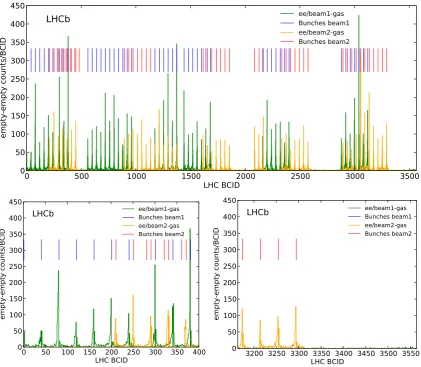
Ghost charges are observed around the nominally filled bunches and are mostly absent further than about 20 slots away from filled bunches.

Ghost charge fractions during LHC luminosity calibration fills are measured in four-minute time bins. For each time bin the ghost charge fraction is evaluated with both counting methods: including and excluding double-counted vertices and applying the corresponding average trigger efficiency of table2. If all charges are evenly spread within their bunch slot, each evaluation would provide a different result before efficiency correction, but the same result after efficiency correction. After efficiency correction the differences between the two evaluations are small. This observation is in agreement with the LDM measurements [40], which show that the ghost charge tends to be spread evenly over all RF buckets of a bunch slot. The LDM information on the charge distribution within the nominally empty bunch slots is not used in the results except for fill 3542 during which the trigger was not configured to perform this measurement. The average of the two efficiency-corrected evaluations is taken as final value for the ghost fraction, while their difference is taken as systematic uncertainty. The trigger efficiency uncertainty taken from table2is added in quadrature with the systematic uncertainty. A summary of all ghost charge measurements performed for the special luminosity fills in 2011, 2012 and 2013 is provided in table3.

2014 JINST 9 P12005

0

500

1000

1500

2000

2500

3000

3500

LHC BCID

0

50

100

150

200

250

300

350

400

450

empty-empty counts/BCID

LHCb

ee/beam2-gas Bunches beam2

0 50 100 150 200 250 300 350 400

LHC BCID 0

50 100 150 200 250 300 350 400 450

empty-empty counts/BCID

LHCb

3200 3250 3300 3350 3400 3450 3500 3550 LHC BCID

0 50 100 150 200 250 300 350 400 450

empty-empty counts/BCID

LHCb

Bunches beam1 ee/beam2-gas Bunches beam2

Figure 4. Histogram of ghost charge distribution as a function of LHC bunch slot number (BCID) in fill 2520 for beam 1 (green) and beam 2 (yellow). The BCID position of nominally filled bunches is indicated as small vertical blue and red lines for beam 1 and beam 2, respectively. The ghost charge distribution is shown for the (top) ring circumference and (bottom left) first 400 and (bottom right) last 400 BCIDs. Ghost charges are mostly absent in regions without nominally filled bunches. Note that onlyeeBCIDs are displayed.

stable within±10% during a fill and the total beam intensity can be corrected with good accuracy using an average value for a fill. In this case the RMS over the fill, given in table3, should be taken into account in the uncertainty. On the contrary, for the intermediate-energy fills, an increase in the ghost charge fraction over time warrants a time dependent correction to the total beam intensity. As an example, the difference in ghost charge evolution seen between high- and intermediate-energy fills is shown in figure5comparing the long fill 2855 at√s=8TeV and fill 3563 at√s=2.76TeV.

3.3 Total uncertainty

2014 JINST 9 P12005

09:00 11:00 13:00 15:00 17:00 Time

0.0 0.1 0.2 0.3 0.4 0.5

Ghost charges fraction (%)

beam 1 beam 2 LHCb

00:00 01:00 02:00 03:00 04:00 Time

0.5 1.0 1.5 2.0 2.5

Ghost charges fraction (%)

beam 1 beam 2 LHCb

Figure 5. Ghost charge fractions for (left) fill 2855 and (right) fill 3563. Fill 2855 with√s=8TeV shows a constant or slightly decreasing ghost charge fraction throughout the fill lasting about 9 hours. Fill 3563 (√s=2.76TeV) shows an important increase of ghost charge over a period of 4 hours.

ghost charge uncertainty on the bunch population product is the linear sum of the ghost charge systematic uncertainty of each beam.

The satellite fractions provided by the LDM [40] are measured at the beginning and at the end of the fill. Here, the average of these two measurements is used. The average satellite fractions for all colliding bunches and fills withβ∗=10 m at√s=8TeV are 0.25% and 0.18% for beam 1 and beam 2, respectively. The uncertainty on the satellite fraction correction is taken as the full differ-ence between the fractions measured at the beginning and end of fill. Assuming the uncertainties are fully correlated between the two beams, the uncertainty on the population product due to the satellite fraction correction is taken as the linear sum of the average uncertainties per beam, and is given as the average per fill in table4.

The beam population product normalization uncertainty is dominated by the DCCT measure-ment. All fills listed in table4are subject to the same procedure to evaluate the beam population product uncertainty. For fills with β∗ =10m and √s=8TeV, the average uncertainty on the bunch population product weighted with the number of measurements amounts to 0.22% at 68% confidence level.

4 Relative luminosity calibration

Absolute luminosity calibrations are performed during short periods of data-taking. To be able to determine the integrated luminosity for any data sample obtained during long periods, the interac-tion rate of standard processes is measured continuously. The effective cross-secinterac-tion corresponding to these standard processes is determined by counting the visible interaction rates during the spe-cific periods when the absolute luminosity is calibrated.

4.1 Interaction rate determination

2014 JINST 9 P12005

Table 3. Measurements of ghost charge fractions for all luminosity calibration fills in 2011, 2012 and 2013. The systematic uncertainty is assumed to be fully correlated between the two beams. Therefore, the final systematic uncertainty on the beam intensity product due to the ghost charge correction is a linear sum of the ghost charge systematic uncertainty of each beam. Proton-lead fills were acquired without neon gas injection and have a larger statistical uncertainty. For fill 3542 the ghost charge was only measured using the LHC LDMs.

Fill Beam 1 Beam 2

fghost,1 RMS uncertainty fghost,2 RMS uncertainty (%) in fill syst. stat. (%) in fill syst. stat. Fills with ppat√s=8TeV

2520 0.30 0.01 0.02 0.001 0.35 0.01 0.01 0.002 2523 0.50 0.02 0.03 0.001 0.44 0.01 0.01 0.001 2852 0.62 0.01 0.04 0.002 0.53 0.01 0.01 0.002 2853 0.40 0.01 0.02 0.002 0.28 0.01 0.01 0.002 2855 0.22 0.01 0.01 0.001 0.23 0.01 0.01 0.001 2856 0.24 0.01 0.01 0.001 0.22 0.02 0.01 0.001 3311 0.15 0.03 0.01 0.001 0.06 0.01 0.01 0.001 3316 0.19 0.01 0.01 0.001 0.06 0.01 0.01 0.001 Fills with ppat√s=7TeV

2234 0.84 0.10 0.05 0.012 0.76 0.13 0.02 0.015 Fills with ppat√s=2.76TeV

3555 0.58 0.14 0.04 0.001 0.33 0.03 0.01 0.001 3562 0.78 0.30 0.05 0.003 0.52 0.22 0.01 0.003 3563 1.28 0.55 0.08 0.002 0.88 0.35 0.02 0.002 Fills with pPb at√sNN=5TeV

3503 0.18 0.04 0.01 0.005 0.50 0.13 0.01 0.011 3505 0.29 0.05 0.02 0.007 0.66 0.12 0.02 0.015 Fills with Pbpat√sNN=5TeV

3537 0.50 0.12 0.03 0.010 0.88 0.11 0.02 0.015 3540 0.73 0.09 0.05 0.019 0.17 0.05 0.01 0.014

3542 n.a. n.a.

interaction rate does not need to have a simple physics interpretation. Any interaction rate that can be measured under stable conditions can be used as such a relative luminosity monitor. The interaction rates are acquired and stored together with the physics data as “luminosity data”. During further processing of the data the relevant luminosity information is kept in the same storage entity. Thus, it remains possible to select only part of the full data set for analysis and still keep the capability to determine the corresponding integrated luminosity.

2014 JINST 9 P12005

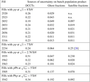
Table 4. Relative uncertainties (in percent) on colliding-bunch population products for all relevant fills. Fill Sources of uncertainty on bunch population product

DCCTs Ghost fractions Satellite fractions Fills with ppat√s=8TeV

2520 0.26 0.029 n.a.

2523 0.22 0.043 n.a.

2852 0.19 0.049 0.097

2853 0.24 0.032 0.019

2855 0.21 0.019 0.021

2856 0.21 0.020 0.031

3311 0.22 0.011 0.011

3316 0.23 0.013 0.011

Fills with ppat√s=7TeV

2234 0.24 0.064 0.25 [28]

Fills with ppat√s=2.76TeV

3555 0.51 0.047 0.230

3562 0.22 0.062 0.020

3563 0.23 0.101 0.024

Fills with pPb at√sNN=5TeV

3505 0.31 0.137 0.070

Fills with Pbpat√sNN=5TeV

3542 0.34 0.192 0.092

with only a beam-2 bunch (eb) and the remaining 5% to slots that are empty (ee). The events taken

for crossing types other thanbbare used for background subtraction and beam monitoring.

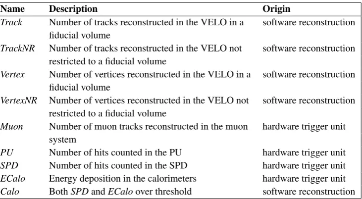
Interaction rates are measured by processing the random luminosity triggers and these rates are stored in a small number of “luminosity observables”. The set of luminosity observables comprises the number of vertices and tracks reconstructed in the VELO, the number of muons reconstructed in the muon system, the number of hits in the PU and in the SPD in front of the calorimeters, and the transverse energy deposition in the calorimeters. The number of vertices in the VELO that fall within a limited region around the nominal interaction point and VELO tracks crossing this region are counted separately. Some of these observables are directly obtained from the hardware trigger decision unit, others are the result of partial event reconstruction in the software trigger or in the off-line software. Observables used in this analysis are summarized in table5.

The luminosity for a given data set can be determined by integrating the values of observables that are proportional to the instantaneous luminosity and by applying the corresponding absolute calibration constant. However, this procedure sets stringent requirements on the stability of the observable and on its linearity in the presence of multiple interactions. Alternatively, one may determine the relative luminosity from the fraction of “empty” or invisible events inbbcrossings

2014 JINST 9 P12005

Table 5. Definition of luminosity observables used in the analysis. The fiducial volume used here is a cylinder of radius<4mm around thezaxis and bound by|z|<300mm. It is used to cut either on the point of closest approach of a track relative to thezaxis or on the position of a vertex.

Name Description Origin

Track Number of tracks reconstructed in the VELO in a software reconstruction fiducial volume

TrackNR Number of tracks reconstructed in the VELO not software reconstruction restricted to a fiducial volume

Vertex Number of vertices reconstructed in the VELO in a software reconstruction fiducial volume

VertexNR Number of vertices reconstructed in the VELO not software reconstruction restricted to a fiducial volume

Muon Number of muon tracks reconstructed in the muon hardware trigger unit system

PU Number of hits counted in the PU hardware trigger unit

SPD Number of hits counted in the SPD hardware trigger unit

ECalo Energy deposition in the calorimeters hardware trigger unit

Calo BothSPDandECaloover threshold software reconstruction

a colliding bunch pair, the number of interactions per bunch crossing follows a Poisson distribution with mean value proportional to the luminosity, hence the luminosity is proportional to −lnP₀. In the absence of backgrounds, the average number of visible ppinteractions per crossing can be obtained from the fraction of emptybb crossings byµ_vis=−lnP₀bb. This “zero-count” method is both robust and easy to implement [41]. The choice of a low visibility threshold ensures a better behaviour under gain or efficiency variations of the observable than the straightforward linear summing method. In addition, any non-linearity encountered with multiple events does not play a role when counting empty slots.

Assuming equal particle populations inbb, be, and ebbunches and no particles in eeslots,

backgrounds are subtracted using

µ_vis=−

lnPbb

0 −lnP0be−lnP0eb+lnP0ee

, (4.1)

wherePi

0(i=bb,ee,be,eb)are the probabilities to find an empty event in a bunch-crossing slot for the four different bunch-crossing types. In eq. (4.1) it is implicitly assumed that all bunches of the same type have the same properties. The consequences of this approximation will be discussed in section4.2. ThePee

0 contribution is added because it is also contained in theP0be andP0eb terms. The purpose of the background subtraction, eq. (4.1), is to correct the count-rate in thebbcrossings

for the detector response, which is due to beam-gas interactions and detector noise. In principle, the noise background is measured duringeecrossings. In the presence of parasitic beam protons

ineebunch positions (ghost charge), it is not correct to evaluate the noise fromP₀ee. In addition,

the detector signals are not fully confined within one 25ns bunch-crossing slot for some of the ob-servables. The empty (ee) bunch-crossing slots immediately following abb,beorebcrossing slot

2014 JINST 9 P12005

LHCb

0 300 600 900

3.5 4.0 4.5 5.0 5.5 6.0 Mean of ECalo counter

W

eighted

number

of

runs LHCb

0 200 400 600

0.000 0.025 0.050 0.075 Mean of Track counter

W

eighted

number

of

runs

Figure 6. Mean value of (left)ECaloand (right)Trackobservables ineecrossings. Each histogram entry

represents the average over a run2 _{in 2012 and is weighted with the corresponding integrated luminosity.}

For measurements using theECaloandCaloobservables we discard the runs for which theECalopedestal mean is lower than 4.75 (dashed vertical line).

slots, the spill-over background is negligible in the bb, be andeb crossings. Since the detector

noise for the selected observables is small (see section4.2) the term lnPee

0 in eq. (4.1) is neglected. The results of the zero-count method based on the number of tracks and vertices reconstructed in the VELO are found to be the most stable. An empty event is defined to have<2 tracks in the VELO. A VELO track is defined by at least threeRclusters and threeφclusters on a straight line in the VELO detector. The number of tracks reconstructed in the VELO restricted to a fiducial region is chosen as the reference observable.

4.2 Systematic uncertainties

The zero-count method is valid if an event is considered empty when the value of the observable is exactly zero. However, if the observable is affected by noise such that its value is never zero, the threshold discriminating empty events has to be increased. This is the case for theECaloandCalo observables, used as a cross-check, for which a positive threshold must be chosen. The introduced bias depends on the noise distribution, the one-interaction spectrum and the average number of interactions per crossing. While the latter was kept approximately constant during the 2012 data-taking period, the Calonoise distribution was changing due to ageing of the hadron calorimeter. In the second half of 2012, the HCAL gain was adjusted more frequently, thus keeping the noise distribution more stable.

The noise distribution is measured ineecrossings. Histograms of the mean value of the noise

are shown for theECaloand theTrackobservable in figure6. For theECaloobservable, two peaks are observed in the pedestal distribution. This is attributed to a change of operating conditions, which is not easily corrected for. Therefore, for cross-checks using theECaloandCalo observ-ables we discard the runs for which theECalopedestal mean is lower than 4.75. The remaining larger fraction of runs spans the full year and is subsequently used for assessment of systematic uncertainties. TheTrackobservable has typically less than 2.5 tracks per 100eecrossings, which

induces a negligible bias. The systematic uncertainty due to noise is negligible.

2014 JINST 9 P12005

LHCb 0.0% 0.1% 0.2% 0.3% 0.4%

115000 120000 125000 130000 Run

Backgr

ound

cor

rection

0 100 200

Figure 7. Beam-gas background fraction −lnPbe

0 −lnP0eb/µ_visfor theTrackobservable during the 2012

running period.

LHCb 1.0000 1.0005 1.0010 1.0015 1.0020

115000 120000 125000 130000 Run

µTrac

kNR

/µT

rac

k

0 100 200 300

Figure 8. Ratio of the measuredµ_vis values without (TrackNR) and with (Track) a fiducial volume cut

during the 2012 running period. The observed deviation from unity is used as an estimate of the systematic uncertainty due to potentially unaccounted background.

Equation (4.1) assumes that the proton populations in thebeandebcrossings are the same as

in thebbcrossings. With a population spread of typically 10% and a beam-gas background fraction

for the reference observable<0.3% compared to theppinteractions (see figure7) the effect of the spread is small and therefore neglected.

The measured µ_vis values can be contaminated by other backgrounds than beam-gas inter-actions, e.g. collisions between satellite and main bunches, and interactions with material in the VELO. We reduce such effects by applying a fiducial volume cut to the Track observable. To assess the magnitude of potentially unaccounted background, a comparison is made between the µ_vis values measured with (Track) and without (TrackNR) the fiducial volume cut, see figure 8. The observed discrepancy is used as an estimate of the systematic uncertainty due to beam-beam background.

2014 JINST 9 P12005

LHCb

−40 −20 0 20 40 60

115000 120000 125000 130000

Run ξlz

(mm)

0 200 400 600

LHCb

10 20 30 40

123600 123700 123800 123900

Run ξlz

(mm)

Figure 9. Longitudinal position of the luminous regionξlzduring the 2012 running period. The bottom plot

shows a subset consisting of a few fills (distinguished with alternating open and solid markers).

and vertices is not uniform alongzat the scale of the observed variations. Therefore, a correction needs to be applied to the observedµ_visvalues that are measured using VELO observables. The Caloobservable is not affected.

From simulation we determineI(0|z), the probability to obtain an empty event while having one interaction atz,

I(0|z)≡P(empty event|one interaction atz), (4.2) see figure10(left). Defining f(z)as the probability density of the longitudinal vertex distribution, the probability ¯I(0|f)to have an empty event while one interaction occurred is

¯

I(0|f) =Z I(0|z)f(z)dz. (4.3) The absolute normalization ofI(0|z)and ¯I(0|f)depends on the underlying interaction generator. However, the normalization does not affect the luminosity measurement if used consistently. To avoid scalingµ_viswith factors largely different from unity, the correction is made with respect to a reference value ¯I(0|ref)that corresponds to a Gaussian probability densityg(z)of the longitudinal vertex distribution centred at zero and having an RMS ofσ_lz=50mm,

¯

I(0|ref) =Z I(0|z)g(z)dz. (4.4) The observed values,µ_visraw, are proportional to 1−I¯(0|f). Thus, the corrected values are given by

µ_vis=1−I(0¯ |ref)

2014 JINST 9 P12005

LHCb simulation

0.5 0.6 0.7

−200 −100 0 100 200

Vertexz(mm)

1

−

I

(0

|

z

)

LHCb simulation 1.00

1.05 1.10

−100 −50 0 50 100

ξlz(mm)

Cor

rection

factor

Track,√s= 2.76 TeV Track,√s= 8 TeV Vertex,√s= 2.76 TeV Vertex,√s= 8 TeV

Figure 10. (Left) probability to see an event given an interaction atz and (right) correction factor as function of the longitudinal positionξlzof the luminous region with sizeσlz=50mm. Only data for one

magnet polarity are shown as it is almost identical to that for the other polarity.

LHCb

0 250 500 750 1000

0% 10% 20% 30%

RMS(µ)/hµi

Number

of

runs

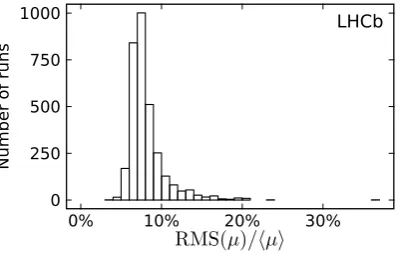
Figure 11. RMS ofµ_visacrossbbbunch crossings relative to the mean value for the 2012 running period.

Thezdistribution of the vertices is well approximated with a Gaussian function. Examples of the correction factors for a Gaussian vertex distribution withσ_lz=50mm are shown in figure10(right).

2014 JINST 9 P12005

bunches. Thus, theµ_visvalue varies acrossbbcrossings. An estimate of the spread ofµ_vis values is the RMS divided by the mean across bunch crossings, as shown in figure11. Due to the non-linearity of the logarithmic function, ideally one first needs to compute µ_vis values for different bunch crossings and then take the average. However, for short time intervals the number of samples is insufficient to make an unbiased measurement per bunch crossing using the zero-count method, whileµ_vismay not be constant when the intervals are too long due toe.g.loss of bunch population and emittance growth.

During physics data-taking, the bandwidth reserved for luminosity triggers is limited. There-fore, a statistically significant measurement of the luminosity cannot be obtained for each bunch crossing individually by integrating over periods shorter than about 30 minutes. The bias and systematic uncertainty introduced by this limitation is evaluated with a simulation. To reflect the luminosity integration for physics data, the number of visible interactions is counted in short time intervals ignoring the spread ofµ_visvalues across bunch crossings. A set of 30 consecutive short intervals is used to accumulate a sufficient number of events per BCID. Then, a correction for the spread is calculated and applied as described below.

For the following discussion backgrounds are not considered since their effect on the correc-tion is negligible. Letnti andkti denote the number of random triggers and the number of empty

events, respectively, inbbcrossing slotiand short time intervalt. Where the indextis omitted, an

implicit sum is assumed over the setT of consecutive short intervals. Similarly, in case the indexi is omitted, a summation over allbbbunch crossings is assumed. A correction factor is calculated

for every setT and is applied to each short periodt∈T

κ_T =h−ln ki nii −lnk

n

, (4.6)

where the average in the numerator is taken overi. The corrected estimate of the number of visible interactions is

Nvis,T=κ_Tftrig

_∑

−ntln_nkt t

, (4.7)

where ftrigis the probability that abbcrossing is randomly triggered.

A simulation study is performed to compare the bias of the estimated number of interactions before and after the correction procedure. The rate of triggers and the number of bunch crossings is chosen to reflect the typical running conditions. Theµ values across bunch crossings are sampled from a normal distribution. A luminosity half-life of two hours is assumed. The bias is calculated as function of meanµ value and relative RMS, and is shown in figure12.

To estimate the residual bias of the correction technique on the data, we perform a simulation for each long periodT. First, the µ_vis value is estimated for each short periodt and each bunch crossingiwith

µ_ti=−ln kt nt ln

ki ni lnk

n

, (4.8)

2014 JINST 9 P12005

-1.2% -0.8% -0.4% 0.0%

0.0 0.5 1.0 1.5 2.0 2.5

hµi

Bias

not corrected corrected

spread 1% spread 8% _-1.2% -0.8% -0.4% 0.0%

0% 4% 8% 12%

RMS(µ)/hµi

Bias

not corrected corrected

hµi= 0.1 hµi= 1.7

Figure 12. Bias of the estimated number of interactions as function of (left) mean µ value and (right)

relative RMS. The bias is fitted with a straight line and an even quadratic polynomial as function ofhµiand

relative RMS, respectively. A quadratically increasing bias as function of relative RMS is present for large

hµivalues before the correction (dashed blue line). For 2012 data taking conditions, the typicalhµifor the

Trackobservable is 1.7 and the typical relative RMS is 8%.

LHCb

0 250 500 750

0% 1% 2% 3% 4%

Correction applied toµ_Track

W

eighted

number

of

runs LHCb

0 250 500 750 1000

-0.2% 0.0% 0.2% 0.4%

Bias due to spread ofµ

W

eighted

number

of

runs

Figure 13. (Left) correction applied to the estimated values ofµ_Trackfor variations of its value across bunch

crossings and (right) residual relative bias of the estimated number of visible interactions after the correction. Each histogram entry represents a run in 2012 and is weighted with the corresponding integrated luminosity.

pair,kti is sampled from a binomial distribution with success probabilitye−µi and number of trials

equal tonti. As for the actual data, eqs. (4.6) and (4.7) are used to estimate the number of visible

interactions. Finally, the bias is obtained from the difference of the estimated and the true number of visible interactions, averaged over 25 independent repetitions of the simulation. Histograms of the average values of κ_T and the residual relative bias for each run are shown in figure13. The relative integrated bias over the full data set is assigned as a systematic uncertainty (0.14%).

2014 JINST 9 P12005

LHCb

0.9475 0.9500 0.9525 0.9550

115000 120000 125000 130000

Run µCalo

/µT

rac

k

0 50 100 150 200

Figure 14. Ratio of the relative luminosities using theTrackand theCaloobservables during the 2012 running period. Only data for runs that are longer than 30min are plotted. The variation of the ratio after subtraction of the variation due to statistical fluctuations is shown with a shaded area spanning±1σaround

the mean.

Table 6. Top: systematic uncertainties of the relative luminosity measurement (in %). Bottom: integrated effect of the applied corrections (in %).

pp pPb Pbp

Source 8TeV 7TeV 2.76TeV 5TeV 5TeV

Beam-beam background 0.13 0.24 0.13 0.95 0.73 Efficiency of the observable 0.19 0.07 0.12 0.09 0.11 Bunch spread 0.14 0.09 0.10 0.03 0.03 Bunch spread (cross-check) 0.09 0.44

Stability 0.12 0.13 0.14 0.39 0.35

Total 0.31 0.53 0.25 1.03 0.82

Correction

Efficiency of the observable −0.54 −0.11 −0.12 −0.09 −0.11 Bunch spread +0.72 +0.99 +0.10 +0.03 +0.03

simulation, the result is taken as an additional systematic uncertainty (0.09%).

The stability of the reference observable is demonstrated in figure 14, which shows the ra-tio of the relative luminosities determined with the zero-count method using the Track and the Caloobservables. These two observables use different sub-detectors and have different system-atic uncertainties. The variation of the ratio unexplained by statistical fluctuations is assigned as a systematic uncertainty to the relative luminosity measured using theTrackobservable. A similar cross-check with the ratio of the relative luminosities using the Trackand theVertexobservables shows negligible discrepancy.

2014 JINST 9 P12005

cross-checks, the full amount of each correction is assigned as an uncertainty. The beam-beam background uncertainty is estimated to be up to 1% for the proton-lead data taking, owing to the very lowµ values (0.01–0.02) of these runs. A higher uncertainty of about 0.5% due to the bunch spread is estimated for the 2011 data taking. This is explained by worse conditions in the begin-ning of the year, when the spread ofµ across bunches reached 30%, which leads to a correction of up to 7% for some fills. The 2011 data taking at 7TeV was affected by parasitic collisions due to a vanishing net crossing angle for one of the magnet polarity settings. This background ranges between 0.2% and 0.7% and a correction is applied averaging over time intervals of a few weeks each, during which data were taken under similar conditions. The average correction amounts to about 0.4% and since only about half of the 2011 running period is affected, an uncertainty due to parasitic collisions of 0.2% is assigned on the full period. In addition, the estimated uncertainty due to beam-beam background from 2012 is added in quadrature to obtain 0.24% uncertainty for 2011. The stability of the effective process is estimated using only data that is not affected by parasitic collisions.

5 Formalism for the luminosity of colliding beams

In a cyclical collider, such as the LHC, the average instantaneous luminosity of one pair of colliding bunches can be expressed as [6]

L=N1N2ν_rev r

|v1−v2|2−|v1×v2| 2 c2

Z

ρ1(x,y,z,t)ρ2(x,y,z,t)dxdydzdt, (5.1) where we have introduced the velocitiesv1 andv2 of the particles (in the approximation of zero emittance the velocities are the same within one bunch). The particle densitiesρ_j(r,t)(j=1,2) at positionr= (x,y,z)and timetare normalized such that their individual integrals over all space are unity at all times. For highly relativistic beams colliding with a small half crossing-angleφ, the Møller factorp

(v1−v2)2−(v1×v2)2/c2 reduces to 2ccos2φ '2c and one recovers eqs. (1.2) and (1.3). The LHCb system of coordinates, which is used here, is chosen as a right-handed cartesian coordinate system with its origin at the nominal interaction point IP8. Thezaxis points towards the LHCb dipole magnet along the nominal average beam-line, thexaxis lies in the hori-zontal plane, withx>0 pointing approximately toward the centre of the LHC ring, and theyaxis completes the right-handed system. This system almost coincides with the LHC coordinate sys-tem. Small angles due to the known LHC plane inclination and other magnetic lattice imperfections have negligible influence on the measurement of the overlap integral as only the crossing angles are relevant, not the individual beam directions.

Up to a normalization factor,ρ_bb(x,y,z,t) =ρ₁(x,y,z,t)ρ₂(x,y,z,t)is the distribution of inter-actions from the luminous region in the laboratory frame. If bothρ₁andρ₂ factorize as a product of a longitudinal and a transverse density (relative to the direction of motion of the bunch), the spatial distribution integrated over time4_{can be expressed as}

ρ_bb(x,y,z) =n(z)ρ₁(x,y,z)ρ₂(x,y,z) (5.2)

4_{When the time dependence is dropped, an integration over time is implied:ρ(x,y,z) =}R

2014 JINST 9 P12005

beam-beam and beam-gas interactions is used in the BGI analysis.

Determining the luminosity or the reference cross-section requires measuring the bunch pop-ulation productsN1N2, as discussed in section3, and evaluating the overlap integralΩ. We briefly describe the principles of the two methods that are used in this paper to determine the latter.

5.1 Beam overlap measurement methods

The first method was introduced by van der Meer to measure the luminosity of the coasting beams at the Intersecting Storage Rings (ISR) [12]. The method was further extended to measure the luminosity of a collider with bunched beams [13] and is the main method used to determine the luminosity at the other LHC experiments. The key principle of the VDM scan method is to express the overlap integral in terms of rates that are experimental observables as opposed to measuring the bunch density functions. Experimentally, the method consists in moving the beams across each other in two orthogonal directions. The overlap integral can be inferred from the rates measured at different beam separations, provided the beam displacements are calibrated as absolute distances.

A reaction rate Rper bunch crossing is measured that is proportional to the luminosity and depends on the two orthogonal transverse separations of the two beams ∆x and∆y. Measuring this rate relative to the revolution frequencyν_rev(approximately 11245 Hz at the LHC) defines the parameter µ, which is the average number of reactions per bunch crossing. In the case where the spatial distributions of the beams can be factorized in the two coordinatesxandy, it is sufficient to measureµ (and thusR) as a function of∆x(at a fixed∆y₀) and as a function of∆y(at a fixed∆x₀). One can show that the interaction cross-section is then given by

σ=

R

µ(∆x,∆y0)d∆x·Rµ(∆x0,∆y)d∆y

N1N2µ(∆x₀,∆y₀) . (5.3) The pair of separation values (∆x₀,∆y₀) is called the working point and is typically chosen to be as close as possible to the point where the luminosity is at its maximum. However, eq. (5.3) is valid for any values of ∆x0 and∆y0. It can be shown that it is also valid in the presence of non-zero crossing angles [14].

The VDM method has the advantage of using a measured rate as its only observable, which is experimentally simple. The experimental difficulties of the VDM method arise mostly from the fact that the beams must be moved to perform the measurement. The exact displacements∆xand ∆yin eq. (5.3) steered by the LHC magnets are calibrated at each interaction point in a so-called length scale calibration (LSC). While the resulting corrections are typically of the order of 1%, some non-reproducibilities have been observed between two consecutive scans without being able to identify the cause. Another difficulty originates from beam-beam effects. When the beams are displaced, a change inβ∗ (dynamic beta effect) and a beam deflection may be produced, which both influence the observed rate. The resulting corrections to the visible cross-section depend on the LHC optics, the beam parameters and filling scheme, and must be evaluated at each interaction point (see section7.6).

2014 JINST 9 P12005

valid at the required precision.

An alternative to the VDM scan method for measuring the luminosity is provided by the BGI method [16], which was first applied at the LHCb experiment in 2009 [21] and 2010 [11]. The principle of this method is to evaluate the overlap integral by measuring all required observables in eq. (1.3) using the spatial distribution of beam-gas and beam-beam interaction vertices. The details of the measurement are discussed in section6. Measuring the shapes of stationary beams avoids changes due to beam-beam effects and other, non reproducible, effects due to beam steering. Furthermore, at the LHC the BGI measurements at a given IP (here at LHCb in IP8) can be made in parallalel to the VDM scans of other LHC experiments and can therefore be made more frequently. On the other hand, while theβ∗and crossing angles used at the LHC do not impact the VDM method to first order, the BGI measurement relies on the vertex measurement to determine the bunch shape. Therefore, an increasedβ∗ is preferable to avoid limitations introduced by the de-tector resolution. At LHCb, in 2012, ppphysics data were acquired atβ∗=3m, while the most precise BGI luminosity calibrations fills were carried out withβ∗=10m. The knowledge of the crossing angle is also important since the luminosity reduction due to the crossing angle has been as large as 20%. A non-vanishing crossing angle is necessary to avoid interactions between the main bunch and out-of-time charges captured in the next RF bucket, which occur nearz=±37.5cm. Such displaced collisions, if present, must be disentangled from beam-gas interactions. They can be completely avoided by introducing a sufficiently large crossing angle. The VDM measurement can exclude interactions occurring away from the interaction point and is therefore less affected by these satellite collisions.

The VDM and BGI methods are complementary, in the sense that their systematic uncertainties on the overlap integral are highly uncorrelated, and a luminosity calibration performed with both methods in the same fill permits their systematic uncertainties to be constrained further. At present this can only be done at the LHCb experiment.

The analyses of the VDM and BGI luminosity calibration measurements presented here indi-cate that the observed luminosity profiles and vertex distributions are not consistent with Gaussian bunch distributions. It is found that a sum of two Gaussian functions (“double Gaussian” shape model) is sufficient to describe thexandyshapes of each bunch as well as the resulting luminous region. However, the joint two-dimensional transverse distribution of the bunches is found to be non-factorizable in the transverse coordinates. Therefore, as explained in section5.3, the transverse shape of the bunches is modelled with a sum of four two-dimensional Gaussian functions, which is in general non-factorizable.

In order to explain the full analysis of the present work, which involves a detailed fit model with a sum of Gaussian terms, it is useful to consider first the formalism for the ideal case of pure Gaussian beams and then describe the two-dimensional (non-factorizable) Gaussian model used in this work.

5.2 Luminosity in the case of purely Gaussian beams

2014 JINST 9 P12005

assumed that the ˆyj axes of the two colliding bunches are parallel to the yaxis of the laboratory

frame. The beam crossing plane, defined by the velocity vectors v1 and v2, is here assumed to coincide with thexzplane. This condition was not respected only for the April 2012 fills. The relevant modifications of the formulae below are discussed in section7.2. We assume the bunches are centred at rj = (ξ_{x j},ξ_{y j},ξ_{z j}) at time t=0, with a particle density function described by a normalized Gaussian function

ρ_{m j}(m) =√ 1 2π σ_{m j}e

−1 2

m−ξ_{m j} σ_{m j}

2

for beam j=1,2 and coordinatem=x,ˆ y,ˆ z,ˆ (5.4)

whereσ_{m j}denotes the RMS of the corresponding Gaussian function.

Assuming thatρ_j(r,t) =ρ_j(r−v_jt,0), one can show that the overlap integral becomes

Ω=e

−∆x2 2Σ2_x−

∆y2 2Σ2_y

2πΣ_xΣ_y , (5.5)

where the following quantities have been introduced

Σ2_x=2σ_z2sin2φ+2σ_x2cos2φ with 2σ_x2=σ_xˆ2₁+σ_x2_ˆ2

Σ2_y=2σ_y2 2σ_y2=σ_yˆ2₁+σ_y2_ˆ2

2σ_z2=σ_zˆ2₁+σ_zˆ2₂

(5.6)

and∆m=ξ_m1−ξ_m2 (withm=x,y) are the transverse beam separations evaluated at the moment t=0 when the colliding bunches are at the samezposition. In the LHCb experiment, thiszposition (calledzrf) is defined by the LHC RF timing and needs not coincide with the locationz=0 of the LHCb laboratory frame nor with the geometrical crossing point of the two beam trajectories.

The longitudinal positionξ_lzof the luminous region is related to the beam separation∆xand longitudinal bunch crossing pointzrfwith

ξ_lz−zrf= sinφcosφ(σ 2

x −σ_z2)

Σ2_x ∆x. (5.7)

The indexlindicates here a property of the luminous region, as opposed to a single beam property. One can also show that the longitudinal sizeσ_lzof the luminous region is related to the con-volved bunch lengthσ_zby

1 σ_lz2 =

2sin2φ σ_x2 +

2cos2_φ

σ_z2 . (5.8)

2014 JINST 9 P12005

5.3 Double Gaussian shape model

A factorizable transverse beam distribution with double Gaussian projections has the density

ρ(x,ˆ y) =ˆ ρ(x)ˆ ρ(y) =ˆ

_∏

m=x,ˆyˆ[wmg(m;

ξ_m,σ_mn) + (1−w_m)g(m;ξ_m,σ_mw)]

=

_∑

ixiy

wixiyg(x;ˆ ξxˆ,σxiˆx)g(y;ˆ ξyˆ,σyiˆy), (5.9)

whereg(m;µ,σ)indicates a normalized Gaussian function of the variablemwith parametersµand σ. By convention, the narrow (n) and wide (w) components in each projection have widthsσ_mn andσ_mw, and weightsw_mand 1−w_m. The weightsw_ixiy in the sum representation are defined as

wixiy= "

wnn wnw wwn www

#

=

"

wxwy wx(1−wy)

(1−wx)wy (1−wx)(1−wy) #

. (5.10)

The wide and narrow components are assumed to have the same mean, as supported by the data. Moreover, it is assumed that the 3-dimensional bunch distribution factorizes in a transverse (ρ(x,ˆ y))ˆ and a longitudinal component, where the latter is modelled with a Gaussian function.

Non-factorizability can be introduced into the model in eq. (5.9) by modifying the weightswixiy from eq. (5.10). For instance, in an extreme case, one can havewnw=wwn=0 andwnn+www=1, which corresponds to a sum of two 2-dimensional Gaussian functions. To allow for a gradual transition between this extreme case and the case of factorizable beams, it is useful to define the weights as a linear combination

"

wnn wnw wwn www

#

= f

"

wxwy wx(1−wy)

(1−wx)wy (1−wx)(1−wy) #

+ (1−f)

"_w x+wy

2 0

0 1−wx+wy 2

#

, (5.11)

where the coefficient f parametrizes the factorizability. In the fully non-factorizable case (f =0) there is no distinction between thexandyweights, thus the parameterswxandwyare (arbitrarily)

combined in a single weight.

As a result of the single beam model from eq. (5.9), the shape of the luminous region and the overlap integral are described by a weighted sum of 16 components. Explicitly, the beam overlap integral is given by

Ω=

_∑

I wI

Ω_I=

_∑

I wixiy,1wjxjy,2

Ω_I, (5.12)

whereIdenotes the set of indicesix,iy,jx,jy, whilewixiy,1andwjxjy,2are the weights from eq. (5.11) for beam 1 and beam 2. Each partial overlap integralΩ_Iis evaluated with eq. (5.5).

6 Beam-gas imaging method