http://wrap.warwick.ac.uk
Original citation:Zhang, Wenjuan, Wang, Wenbin and Gang, Yi (2013) Maintenance strategy optimisation for infrastructure assets through cost modelling. Working Paper. Coventry, UK:
University of Warwick, WBS. (WBS Working Paper).
Permanent WRAP url:
http://wrap.warwick.ac.uk/57720
Copyright and reuse:
The Warwick Research Archive Portal (WRAP) makes this work by researchers of the University of Warwick available open access under the following conditions. Copyright © and all moral rights to the version of the paper presented here belong to the individual author(s) and/or other copyright owners. To the extent reasonable and practicable the material made available in WRAP has been checked for eligibility before being made available.
Copies of full items can be used for personal research or study, educational, or not-for-profit purposes without prior permission or charge. Provided that the authors, title and full bibliographic details are credited, a hyperlink and/or URL is given for the original metadata page and the content is not changed in any way.
A note on versions:
The version presented here is a working paper or pre-print that may be later published elsewhere. If a published version is known of, the above WRAP url will contain details on finding it.
Corresponding author: Wenjuan Zhang Tel: +44 (0) 24 765 24276
1
Maintenance strategy optimisation for infrastructure assets through cost modelling
Wenjuan Zhanga* , Wenbin Wangb and Gang Yic
a
ORMS Group, Warwick Business School, University of Warwick, Coventry CV4 7AL, UK [email protected]
b
Dongling School of Economics and Management, University of Science and Technology Beijing, China, [email protected]
c
Centre for Process Analytics and Control Technology, University of Strathclyde, Glasgow G1 1XL [email protected]
Abstract. In infrastructure asset management, maintenance strategies in terms of cost modelling is normally adopted to achieve two broad strategic objectives: to ensure that sufficient funding is available to maintain the portfolio of assets; and to ensure that a minimum cost is achieved while maintaining safety. The data and information required for carrying out cost modelling are often not sufficient in quantity and quality. Even if the data is available, the uncertainty associated with the data and the assessment of the assets’ condition remain a challenge to be dealt with. We report in this paper that cost modelling can be carried out at the initial stage instead of delaying it due to data insufficiency. Subjective experts’ knowledge is elicited and utilised together with some information which is gathered only for a small sample of assets. Linear Bayes methods is adopted to combine the sample data with the subjective experts’ knowledge to estimate unknown model parameters of the cost model. We use a case study from the rail industry to demonstrate the methods proposed in this paper. The assets are metal girders on bridges from a rail company. The optimal maintenance strategy is obtained via simulation based on estimated model parameters.
Keywords: maintenance, infrastructure asset, cost modelling, Bayes linear estimator, elicitation, metal girder
1. Introduction
2
For the case study of a rail company considered in this paper, it is estimated that billions of pounds are required to maintain its bridges and structures asset portfolio over the next 50 years. In order to maintain a large number of assets within the bridges and structures portfolio as economically and efficiently as possible, the company needs to optimise the maintenance strategy for its assets. Cost models can help to identify the optimal maintenance strategy for the assets, and have attracted a great deal of attentions from infrastructure industries [1], including rail industry [2], water and environment [3], bridges [4], building and civil infrastructure[5, 6]. Of course, maintaining safety is of utmost importance for these assets, but it is also crucial to maintain these assets in a cost-effective way with a good healthy working order. The consequence of any disruption of a normal service is severe. The cost of maintaining these long-life assets is huge, but cost models, when properly developed, can help to identify the optimal maintenance strategy with the least cost, so the benefit of applying cost models is substantial.
Although there are general interests from the industries on optimising maintenance strategies through cost modelling, the development and application have not advanced much over the
years. There remain many challenges to overcome, as demonstrated in Skinner et al[2].
Among the challenges in rail industry, the key challenges include:
Defining the size and configuration of the asset. The asset should be analysed and any
sub-asset hierarchy down to a maintainable item (MI) should be specified. Such MI is the base unit for planning and executing the required maintenance. For example, a single span bridge constructed of concrete deck with masonry jack arches on metal girders with masonry end supports is defined with five MI’s, each with its own degradation rate, cost and intervention cycles.
Lack of history data in defining asset relationships. The timing of different
interventions is required for optimising maintenance strategy, together with the capital and operational expenditure costs for the range of interventions. Ideally, these information should be based on the assets’ history failure and maintenance data.
3
will take many man hours to obtain the required information from all these paper records.
Dealing with uncertainty. Even if the current conditions of all the assets were known,
it would not be possible to predict future investment costs with certainty.
It is therefore acknowledged that a statistical estimation of costs is needed. Detailed information would be gathered by investigating only a small sample of assets. However, it would be wrong to treat those as the only source of information. Although the company might not know the detailed status of all its assets, a large amount of general and local knowledge and expertise is inevitable acquired in routine data collection practices. Such information does not come in the form of statistical data, in the classical sense of random variables with identifiable sampling distributions, but is a rich source of information. The information in the form of expert knowledge proves to be useful in asset management when the history data is not available. Wang and Zhang [7] utilised expert knowledge to predict asset’s residual life when the history data is lacking in both quantity and quality. Because of the subjective element of expert opinions, the elicitation and the use of expert knowledge should be done carefully. O’Hagan [8] considered the practical elicitation of expert beliefs through two contrasting examples, Garthwaite and O’Hagan [9] reported an experimental study of quantifying expert opinion in the UK water industry, and Wang [10] commented on expert elicitation for reliability system design.
O’Hagan et al [11] have adopted the background knowledge of experts when making asset
management plans. Some sample data are collected and linear Bayes methods are used to combine the sample data with the experts’ knowledge to estimate the costs of the interventions for each asset, and also the timings of the various interventions. However these two kinds of uncertain quantities were dealt with separately, and there was no attempt of combining the uncertainties of costs and timings to predict capital investment.
This paper shall address the problematic issues associated with data and uncertainty when carrying out the cost model. The contributions are:
First, we deal with the lack of available history data issue by investigating only a
4
techniques to extract experts’ knowledge of general and local knowledge and
expertise based on their experience gained from routine data collection practices.
Second, unlike previous applications, we treat both intervention timing and costs as
uncertain. We then adopt linear Bayes methods to combine the sample data with the experts’ knowledge, to make estimates that use all available information.
Third, we build asset cost model based on these estimates, identify the optimal
maintenance strategy and estimate the penalty of delaying maintenance when funding is not sufficient.
The rest of the paper is organised as follows: Section 2 introduces the methodology. Section 2.1 describes and formulates the problem, and defines different maintenance scenarios and strategies. The asset cost model is based on the distribution of both intervention cost and time duration of a MI in each condition, which is described in Section 2.2. Section 2.3 briefly introduces the Bayesian linear estimator, which is adopted to estimate the parameters of intervention cost and time duration of each condition for the cost model. The prior distribution is assumed to be lognormal and is described in Section 2.4. The elicitation process is explained in Section 2.5. Section 3 gives a brief description of the case problem. The intervention cost and time duration estimation is explained in Section 4. The elicited data from the expert knowledge is presented in Section 4.1. In Section 4.2, the posterior estimates and posterior distribution of intervention cost and time duration are obtained through Bayesian linear estimator. The results of the cost model are given for various maintenance strategies through simulation in Section 5, and the penalty of delaying maintenance is estimated. Section 6 presents the modelling validation. Finally a conclusion is made in Section 7 based on the analysis with the recommended optimal maintenance strategy.
2. Methodology
2.1 Problem formulation
5
of a MI, e.g. allowing the item to drop to condition 2 then bring it back to condition 1, or letting the item to deteriorate to condition 4 then bring it back to condition 2, and etc. If we
define as the maintenance scenario, where j=1, 2, 3, 4 is the condition that the MI is in
before it is maintained, and i=1, 2, 3 is the condition after maintenance. Table 1 includes a
full list of possible maintenance scenarios.
Table 1 Maintenance scenarios
Scenario Condition evolution Notes
C1-C2-C1-C2 Back to condition 1 when found in condition 2
C1-C2-C3-C1-C2-C3 Back to condition 1 when found in condition 3
C1-C2-C3-C2-C3 Back to condition 2 when found in condition 3
C1-C2-C3-C4-C1-C2-C3-C4 Back to condition 1 when found in condition 4
C1-C2-C3-C4-C2-C3-C4 Back to condition 2 when found in condition 4
C1-C2-C3-C4-C3-C4 Back to condition 3 when found in condition 4
Based on the different maintenance scenarios, there can be six maintenance strategies. We use to denote the various strategies, which means to carry out the standard intervention
when the condition is equal to or above j, and bring the MI back to the start of condition i.
Where , it is possible that the MI has deteriorated to a condition which is worse than
j at the inspection time.
Strategy 1: Carry out the standard intervention when condition is equal to or above 2, and bring the item back to the start of condition 1. This strategy includes the maintenance
scenarios , , and , we use to denote this strategy.
Strategy 2: Carry out the standard intervention only when condition is equal to or above 3, and bring the item back to the start of condition 1. This strategy includes the maintenance
scenarios , and , we use to denote this strategy.
Strategy 3: Carry out the standard intervention only when condition is equal to or above 3, and bring the item back to the start of condition 2. This strategy includes the maintenance
scenarios and , we use to denote this strategy.
Strategy 4: Carry out the standard intervention only when condition is equal to or above 4, and bring the item back to the start of condition 1. This strategy only includes the
6
Strategy 5: Carry out the standard intervention only when condition is equal to or above 4, and bring the item back to the start of condition 2. This strategy only includes the
maintenance scenario , we use to denote this strategy.
Strategy 6: Carry out the standard intervention only when condition is equal to or above 4, and bring the item back to the start of condition 3. This strategy only includes the
maintenance scenario , we use to denote this strategy.
Due to the availability of funding for asset maintenance, any of these strategies could have been adopted. But the question is what is the optimal maintenance strategy and how often should the item be inspected? We are hoping that the cost modelling will provide a means to
answering these questions. We define the duration for a MI to stay in condition j as , and
is the pdf of the time duration in condition j. is the time duration from the start of
condition i to the end of condition j. We use to denote the pdf of the time duration
from the start of condition i to the end of condition j, which is the convolution of
for j>i. For i=j, we have which is the pdf of the time duration in condition
j. is the cost of intervention for bringing the item back to the start of condition i when it is
in condition j for . We define T as the inspection interval, Cs as the cost of inspection,
and as the cost of the item in condition 5, which can be a high penalty cost.
Let denote the condition at inspection time . For strategy , the probability that a MI
deteriorates to condition j or above at epoch [ ] is
{ }. (1)
If we know and , the probability that a MI deteriorates to condition j at epoch
[ ] becomes
∫ ( ) . (2)
Similarly, the probability that a MI deteriorates to condition j+1 at epoch [ ] can be
written as
∫ ∫ ( ) . (3)
And the probability that a MI deteriorates to condition 4at epoch [ ] can also be
written as
∫ ∫ ( ) . (4)
The probability that a MI deteriorates to the safety critical condition 5at epoch [ ] is
7 when this happens, a high penalty cost will incur.
2.2 The cost model
Once we have the distributions of the intervention cost and the time duration of each condition, we can produce the maintenance cost model. The optimal inspection interval can be identified, as well as the least unit time cost under different maintenance strategies. An intervention cycle is defined as the time interval between two interventions. Expected intervention cycle cost and the expected intervention cycle length can be formulated for each strategy shown above.
The intervention cycle cost under strategy is
1 ) 1 ( 0 4 ) 1 ( 0 ) 1 ( ) 1 ( ) 1 ( ) )) ( 1 )( ( ) ( ) ( ... )) ( 1 )( ( ) ( ) ( )) ( 1 )( ( ) ( ) ( ) ( ) , ( 4 3 ) 1 ( 1 1 ) 1 ( 1 ) 1 ( 1 4 1 ( 1 n nT T n y x nT X X X s i nT T n x nT X X X s j i nT T
n X X
s ij nT
T
n X X
f iJ dydx y x nT F y f x f C C dydx y x nT F y f x f C C dx x nT F x f C C dx x nT F x f C G T EIC j j j j j j j j j
. (6)
The intervention cycle length is
1 ) 1 ( 0 ) 1 ( 0 ) 1 ( ) 1 ( 0 )) ( 1 )( ( ) ( ... )) ( 1 )( ( ) ( )) ( 1 )( ( ) ( ) ( ) ( ) , ( 4 3 ) 1 ( 1 1 ) 1 ( 1 ) 1 ( 1 4 ) 1 ( 1 n nT T n y x nT X X X nT T n x nT X X X nT Tn X X
nT
T
n X X
x nT iJ dydx y x nT F y f x f T dydx y x nT F y f x f T dx x nT F x f T dydx y f x f y x G T EIL j j j j j j j j j
. (7)
The expected cost per unit time for Strategy is
) , ( ) , ( ) , ( iJ iJ iJ G T EIL G T EIC G T
ECT . (8)
8
} ) , (
) , ( , , min{ ) ,
( * *
iJ iJ iJ
iJ
G T EIL
G T EIC G T G
T . (9)
2.3 Bayesian linear estimator
The Bayes linear estimator (BLE) is adopted to estimate the parameters of intervention cost and time duration of each condition for the cost model given in Equations 6-9.
Suppose we have two random vectors X and Y, the BLE of X after observing Y=y is
( ) (10)
and its dispersion matrix is given by
(11)
is the prior mean of X, and is the posterior estimate of X, is a
posterior analogue of the prior variance matrix . The intuitive meaning of Equations
10 and 11 is to update the initial estimate of E(X) by considering the difference between the
newly observed Y and its mean with the covariance matrix. The BLE analysis requires first-
and second-order moments, i.e. , and . If the joint distribution of X and
Y is multivariate normal, then is exactly the posterior mean of X and is the
posterior variance. O’Hagan et al. [11] interprets the BLE and its dispersion as
approximations to posterior mean and variance when the distribution of X and Y is not far
from normal.
2.4Prior
First we need to obtain the prior distributions of intervention cost and time duration of each condition. Since both quantities are usually positively skew distributed, the prior distribution is assumed lognormal for both intervention cost and time duration of each condition,
. (12)
9
understood by the engineers in the form of prior estimates and its deviations. Their judgement is often based much more on data than on personal judgement.
2.5 Elicitation of expert knowledge
The elicitation process is mainly informed judgement, and because of its subjective nature it is important that it is done carefully. For prior expectations of intervention cost and time
duration of each condition we ask the experts for an estimate M which is the mean of X, then
we ask for the upper and lower limits, U and L of X. The limits are chosen to be the one-third
limits, such that X has a third of chance lying within the limits. Our experiences prove that
the one third limits are easily understood by the engineers. Since both quantities are
positively skewed and assumed lognormal distributed, U-M will be larger than M-L, if the
ratios U/M and M/L are roughly equal, we can calculate the mean and standard deviation, which involves the exponential and natural logarithm function. Define
{ ( )} , (13)
where is the interquantile range for the standard normal distribution, equals 0.8416 for
33% to 67% quantile.
Then
mean of , (14)
and standard deviation of √ . (15)
Variances and covariance are elicited by using a variance components approach. Both intervention cost and time duration of each condition are stratified by condition and the variance components were elicited for each stratum separately. Strictly, there are three variance components in such cases. They are the variability of the grand mean, the variability of stratum means around the grand mean and the variability of individual values around their respective stratum means.
10
3 Case problem
In order to maintain the large number of MIs within the bridges and structures portfolio as economically and efficiently as possible, cost models are developed and applied to its top assets in a rail company. In this paper, we use one MI on the bridges – the girders, as an example to illustrate the cost model. To maintain safety, the metal girders on bridges are painted at regular interval depending on its condition, conditions are classified as 1 to 5 based on the extent and severity of the defect, such as peeling, rusty or corrosion. Condition 1 is defined as less than 1% area of peeling with no rusty, condition 2 as 1-5% of peeling and no rusty, condition 3 as 5-15% of peeling and possibly some rusty, and condition 4 as 15-30% of peeling normally with rusty and possibly some corrosion. If there are more than 30% area of defect including peeling, rusty and corrosion, the girder is in condition 5 which is a safety critical condition. A metal girder could move from condition 4 to condition 5 within a year in which case the rule suggests intervening any items identified as in condition 4 before the end of the year to maintain safety. There are generally two types of painting, general painting and vulnerable painting, both can happen at any time before a girder reaches condition 5. But in reality, general painting only happens when the item reaches condition 3 or 4. In this case, the whole girder will be cleaned and repainted. Generally the girder will be brought back to the start of condition 1 with no defect after general painting. The cost of general painting is associated with the size of the item. Vulnerable painting is to paint those vulnerable areas only. After the painting the girder can be in any one condition of conditions 1 to 3, and the cost of vulnerable painting is affected by both the size and the vulnerable area of the item. There are six maintenance scenarios for painting as demonstrated in Table 1.
4 Time duration and cost estimation
4.1Expert knowledge elicitation
11
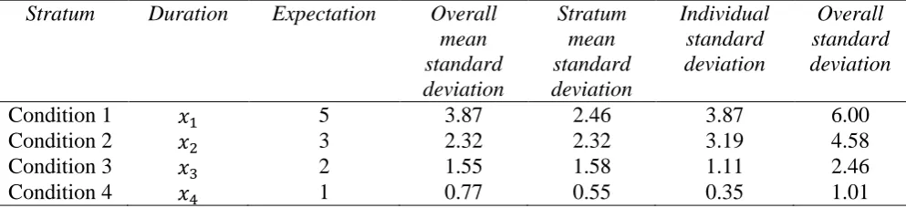
Table 2 Elicited data for duration
Stratum Duration Expectation Overall mean standard deviation
Stratum mean standard deviation
Individual standard deviation
Overall standard deviation
Condition 1 5 3.87 2.46 3.87 6.00
Condition 2 3 2.32 2.32 3.19 4.58
Condition 3 2 1.55 1.58 1.11 2.46
Condition 4 1 0.77 0.55 0.35 1.01
The engineers believe that, after general painting, the girder stays in condition 1 for 5 years on average. For those fall in condition 4, it should be painted within one year to be brought back to a better condition. Prior estimates of conditions were based on recent inspections and may draw on records of any recent intervention.
The elicitation of cost is more complicated as we have mentioned in Section 3 that there are two types of painting and six different maintenance scenarios. These result in six intervention costs, one for each scenario. These costs might be correlated but cannot be directly calculated. Each of the six intervention costs needs to be elicited. Both general and vulnerable painting costs are made of equipment cost, material cost, labour cost, and possibly possession cost. Since painting is a standard intervention, we assume it can be well planned ahead. Any possession costs could be avoided, and we are not going to consider this cost here. Equipment cost is usually not linked with the size of the item, but the type of the painting. This cost is higher for general painting than vulnerable painting. Material cost and labour cost are affected by the area needs to be painted, more so for vulnerable painting than general painting.
The painting cost can be defined as
√ , (16)
where s is the size of the painted area, u is equipment cost, v is unit material cost, and w is
unit labour cost. u, v, and w are assumed to follow lognormal distributions, and are different
for general and vulnerable painting. Instead of eliciting the six intervention costs, we could elicit u, v, and w with two stratum: general painting and vulnerable painting. The various
12
and w doesn’t only reduce the number of quantities for elicitation, it also simplifies the
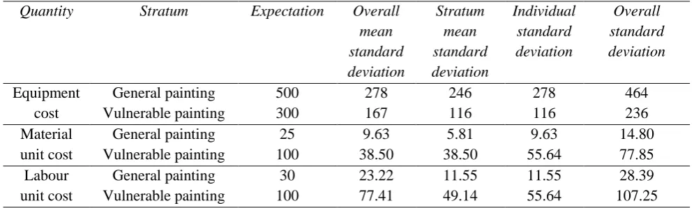
[image:13.595.49.547.238.387.2]elicitation process as the correlations among the original six intervention costs are more complicated to handle. The elicited expectations and standard deviations of costs are shown in Table 3. Again the variation of the costs is elicited using the variance component approach, and the overall standard deviation is made of overall systematic error, stratum error and random error.
Table 3 Elicited data for costs
Quantity Stratum Expectation Overall mean standard deviation
Stratum mean standard deviation
Individual standard deviation
Overall standard deviation
Equipment cost
General painting 500 278 246 278 464
Vulnerable painting 300 167 116 116 236
Material unit cost
General painting 25 9.63 5.81 9.63 14.80
Vulnerable painting 100 38.50 38.50 55.64 77.85
Labour unit cost
General painting 30 23.22 11.55 11.55 28.39
Vulnerable painting 100 77.41 49.14 55.64 107.25
13
Figure 1 Prior deterioration duration distribution
4.2 Posterior
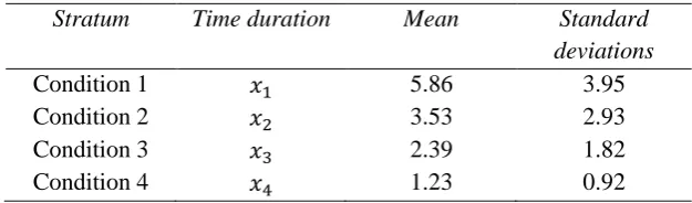
A sample of bridges from different conditions has been studied. Information about the size, condition, maintenance history of the metal girders is collected. Bayesian linear estimator is used to create posterior distributions to refine the prior model using the actual input data from the sample studies. The posterior means and standard deviations for the time duration are given in Table 4.
Table 4 Posterior means and standard deviations for time duration
Stratum Time duration Mean Standard deviations
Condition 1 5.86 3.95
Condition 2 3.53 2.93
Condition 3 2.39 1.82
Condition 4 1.23 0.92
0
5
10
15
0 5
10 15
0 0.2 0.4 0.6 0.8 1
Deterioration duration Prior duration distribution
Age
D
u
ra
ti
o
n
d
is
tr
ib
u
ti
o
[image:14.595.140.453.608.700.2]14
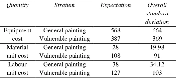
[image:15.595.145.450.181.317.2]The studies revealed that the time durations in all conditions are longer than the engineers’ prior estimates. The updated intervention costs are given in Table 5, which are also bigger than the engineers’ prior estimates, and more variable.
Table 5 Posterior means and standard deviations for costs
Quantity Stratum Expectation Overall standard deviation
Equipment cost
General painting 568 664 Vulnerable painting 387 369 Material
unit cost
General painting 28 19.98 Vulnerable painting 108 91 Labour
unit cost
General painting 38 34.12 Vulnerable painting 127 103
The painting cost is defined in Equation (16), and we assume
̅ , (17)
̅ , (18)
̅ , (19)
then we have
( ̅ ̅ ̅ ), (20)
15
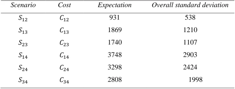
Table 6 Posterior means and standard deviations of costs for painting a 100 meter girder according to
various intervention scenarios
Scenario Cost Expectation Overall standard deviation
931 538
1869 1210
1740 1107
3748 2903
3298 2424
2808 1998
5 Cost model simulation results
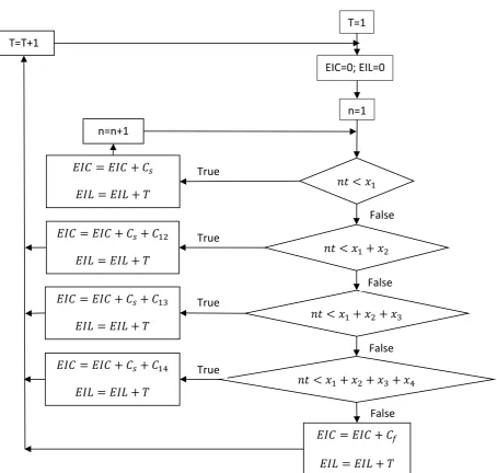
Now we have the distributions of intervention cost and time duration of each condition, we can produce the maintenance cost model. However, in this case study we did not use the analytical procedure given in Equations 6-9 to calculate the expected cost per unit time for each strategy. Instead we use simulation as a way to approximate Equation 8 for the company since Equations 6 and 7 are difficult for the engineers to understand. The analytical procedure also requires longer computation time and bigger computation power because of the convolutions and integrations involved. There are a large number of items within the company, and the computation work is huge, so simulation is a practical solution instead of the analytical procedure.
16
Figure 2 Simulation algorithm
T=1
EIC=0; EIL=0
n=1
𝑛𝑡 𝑥
𝑛𝑡 𝑥 𝑥
𝑛𝑡 𝑥 𝑥 𝑥
𝑛𝑡 𝑥 𝑥 𝑥 𝑥 False
False False
𝐸𝐼𝐶 𝐸𝐼𝐶 𝐶𝑓
𝐸𝐼𝐿 𝐸𝐼𝐿 𝑇 False 𝐸𝐼𝐶 𝐸𝐼𝐶 𝐶𝑠 𝐶
𝐸𝐼𝐿 𝐸𝐼𝐿 𝑇
True 𝐸𝐼𝐶 𝐸𝐼𝐶 𝐶𝑠 𝐶
𝐸𝐼𝐿 𝐸𝐼𝐿 𝑇
True 𝐸𝐼𝐶 𝐸𝐼𝐶 𝐶𝑠 𝐶
𝐸𝐼𝐿 𝐸𝐼𝐿 𝑇
True 𝐸𝐼𝐶 𝐸𝐼𝐶 𝐶𝑠
𝐸𝐼𝐿 𝐸𝐼𝐿 𝑇
True n=n+1
17
Table 7 Simulation results
Strategy 1 2 3 4 5 6
Optimal inspection
interval
22
months 8 months 7 months 3 months 2 months 2 months
Expected unit time cost (sd)
£252 (£181)
£393 (£241)
£870
(£723) (£740) £812 (£950) £1336 (£2566) £2365
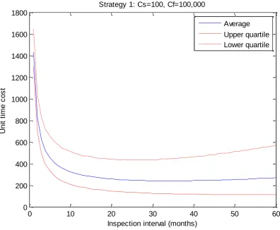
It is clear that Strategy 1 has the smallest expected unit time cost, so it seems that maintaining the item in a good condition is the most cost effective strategy. The optimal inspection interval is about 22 months for Strategy 1 but not sensitive, as shown in Figure 5, the average unit time cost around the area of the optimal interval varies a little with low uncertainties. For other strategies, this area is much smaller and the unit time cost is higher and much more uncertain. The cost curves of other strategies are given in Figures 4-8.
Figure 3 Unit time cost for different inspection intervals for Strategy 1
0 10 20 30 40 50 60
0 200 400 600 800 1000 1200 1400 1600 1800
Strategy 1: Cs=100, Cf=100,000
Inspection interval (months)
U
n
it
t
im
e
c
o
s
t
[image:18.595.89.486.401.727.2]18
Figure 4 Unit time cost for different inspection intervals for Strategy 2
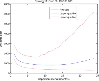
Figure 5 Unit time cost for different inspection intervals for Strategy 3
0 5 10 15 20 25
0 500 1000 1500 2000 2500 3000
Strategy 2: Cs=100, Cf=100,000
Inspection interval (months)
U
n
it
t
im
e
c
o
s
t
Average Upper quartile Lower quartile
0 5 10 15 20 25
0 1000 2000 3000 4000 5000 6000 7000
Strategy 3: Cs=100, Cf=100,000
Inspection interval (months)
U
n
it
t
im
e
c
o
s
t
[image:19.595.119.460.430.707.2]19
[image:20.595.116.459.451.724.2]Figure 6 Unit time cost for different inspection intervals for Strategy 4
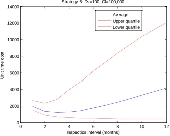
Figure 7 Unit time cost for different inspection intervals for Strategy 5
0 2 4 6 8 10 12
0 1000 2000 3000 4000 5000 6000 7000
Strategy 4: Cs=100, Cf=100,000
Inspection interval (months)
U
n
it
t
im
e
c
o
s
t
Average Upper quartile Lower quartile
0 2 4 6 8 10 12
0 2000 4000 6000 8000 10000 12000 14000
Strategy 5: Cs=100, Cf=100,000
Inspection interval (months)
U
n
it
t
im
e
c
o
s
t
20
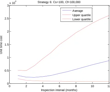
Figure 8 Unit time cost for different inspection intervals for Strategy 6
If the current funding is not sufficient to maintain the item according to the most cost efficient strategy, the natural thing to do will be to delay the painting until further funding becomes available. If the decision was to follow Strategy 6, which is to delay the painting until the item reaches condition 4, and then only carry out the minimum repair, the expected unit time cost will be about nine times of the optimal Strategy 1. Due to the uncertainties of intervention cost and time duration of each condition, the cost model estimates are uncertain. This uncertainty can be reduced once more information is collected where linear Bayes methods can be useful in incorporating new information to update the estimates.
6 Validation
The items can be classified into different groups according to their location and environment. The inspection cost and penalty cost differ as well. Items with easy access will need less
0 2 4 6 8 10 12
0 0.5 1 1.5 2 2.5
3x 10
4 Strategy 6: Cs=100, Cf=100,000
Inspection interval (months)
U
n
it
t
im
e
c
o
s
t
Average
21
[image:22.595.85.529.162.311.2]inspection cost, busy and important lines will result in high penalty costs. Rural location requires higher inspection cost, but probably less penalty involved.
Table 8 Items’ grouping according to their location and environment
=10000 =100000 =1000000
=£100 Easy access, low
importance
Easy access,
medium importance
Easy access, high importance
=£150 Medium access, low
importance
Medium access,
medium importance
Medium access, high importance
=£200 Difficult access, low
importance
Difficult access,
medium importance
Difficult access,
high importance The simulations have been run for items from different groups to calculate the expected cost per unit time. The results are given in Table 9. Strategy 1 still remains optimal for items from all groups, which gives the least expected unit time cost with the smallest uncertainty, and requires least frequent inspection compared to the other strategies. The results for Strategy 1 with various inspection and penalty costs are plotted in Figures 9 and 10. For all strategies, when the penalty increases, the optimal inspection interval decreases; and when the inspection cost increases, the optimal inspection interval increases in general.
Table 9 Simulation results of various penalty and inspection costs
Penalty cost (£)
Inspection
cost (£) Strategy
1 Strategy 2 Strategy 3 Strategy 4 Strategy 5 Strategy 6 10,000
100 24 months
£248 17 months £327 21 months £704 10 months £562 7 months £938 6 months £1876
200 31 months
£279 20 months £387 22 months £755 13 months £666 11 months £1077 8 months £2039 100,000
100 22 months
£252 8 months £393 7 months £870 3 months £812 2 months £1336 2 months £2365
200 23 months
£306 11 months £473 8 months £989 3 months £1216 3 months £1592 2 months £2974 1,000,000
100 15 months
£279 7 months £416 4 months £1043 2 months £1032 1 month £1930 2 months £2720
200 15 months
[image:22.595.77.572.519.767.2]22
Figure 9 Results for Strategy 1 with various penalty costs and low inspection cost
Figure 10 Results for Strategy 1 with various penalty costs and high inspection cost
To validate the results from the posterior estimates, the simulation has been carried out using the prior estimates. The comparison of the results for Strategy 1 is shown in Table 10. The results from the prior estimates tend to be more conservative, which is understandable as the engineers are cautious when making judgements. The sample data proves that the inspection interval can be longer than that the engineering expected, and the unit time cost is cheaper than that expected. And the results from the posterior estimates are less uncertain compared with the prior estimates. This uncertainty can be further reduced once more information is
200 2000 20000
0 10 20 30 40 50 60
Unit
tim
e
c
o
st
Inspection interval (months)
Strategy 1: Cs =£100
Cf=£1,000,000
Cf=£100,000
Cf=£10,000
200 2000 20000
0 10 20 30 40 50 60
Unit
tim
e
c
o
st
Inspection interval (months)
Strategy 1: Cs =£200
Cf=£1,000,000
Cf=£100,000
[image:23.595.124.489.342.565.2]23
[image:24.595.71.556.176.397.2]collected by using linear Bayes methods in incorporating new information to update the estimates. The comparison of results for Strategy 1 with various inspection and penalty costs are also shown in Figures 11-13.
Table 10 Simulation results using Prior and Posterior estimates for Strategy 1
Penalty cost (£)
Inspection cost (£)
Optimal inspection interval Expected unit time cost (sd)
Prior estimates
Posterior
estimates Prior estimates
Posterior estimates
10000
100 17 months 24 months £475 (£479) £248 (£183)
200 22 months 31 months £522 (£514) £279 (£194)
100000 100 6 months 22 months £629 (£541) £252 (£181)
200 9 months 23 months £690 (£664) £306 (£287)
1000000
100 5 months 15 months £675 (£553) £279 (£180)
200 5 months 15 months £913(£553) £360 (£182)
Figure 11 Comparison between prior and posterior results for Strategy 1 with low inspection cost and low penalty cost
0 200 400 600 800 1000 1200 1400 1600 1800
0 10 20 30 40 50 60
Unit
co
st
Inspection interval (months)
Strategy 1: Cs =£100; Cf=£10,000
[image:24.595.92.518.178.648.2]24
Figure 12 Comparison between prior and posterior results for Strategy 1 with low inspection cost and medium penalty cost
Figure 13 Comparison between prior and posterior results for Strategy 1 with high inspection cost and high penalty cost
7 Conclusion
In this paper, we have demonstrated that maintenance cost modelling can be carried out even when there is only limited information and data available for the asset’s condition and
maintenance history. The cost modelling is made possible at the initial stage by eliciting
0 1000 2000 3000 4000 5000
0 10 20 30 40 50 60
Unit
co
st
Inspection interval (months)
Strategy 1: Cs=£100; Cf=£100,000
Prior
Posterior
0 10000 20000 30000 40000
0 10 20 30 40 50 60
Unit
co
st
Inspection interval (months)
Strategy 1: Cs=200; Cf=£1,000,000
Prior
[image:25.595.125.488.362.583.2]25
experts’ knowledge, and only utilising a sample of assets. Bayesian linear estimator has been
very useful in combining the expert opinion and the sample data to estimate the parameters of intervention cost and time duration of each condition, which are important for the cost model. Even when the maintenance information systems can provide detailed information needed for cost modelling, Bayesian methods are still useful in updating the estimates when new information becomes available. The simulation results show that the cost model can identify the optimal inspection interval, and the optimal maintenance strategy with the least unit time cost. If the current funding is insufficient to cover the optimal maintenance plan, cost models can estimate the future cost of recovering the degraded asset condition. For the case study, the cost models developed for its top assets are currently implemented in this rail company. It proved to be very useful in assisting their strategy making, the results are updated regularly whenever new information comes in using Bayesian methods.
Due to practical limitations in this case study, simulation has been used to calculate the expected cost instead of the analytical procedure. In future work, the analytical approach will be used to calculate the results and compared to that of the simulation. The discount rate for the expected cost in the future will also be taken into account. In this paper, only one type of items with one type of intervention is studied. Further work will be carried out to study the optimal maintenance strategy when there are multiple items involved and each potentially with more than one type of interventions.
References
[1] Michie D. Whole life costing: completing the analysis: asset investment strategies, Business planning and financing for infrastructure companies. The Asset Management Conference; 2011.
[2] Skinner M, Kirwan A, Williams J. Challenges of developing whole life cycle cost models for network rail’s top 30 assets. The Asset Management Conference; 2011.
[3] Roebuck R., Dumbrava OD, Tait S. Whole life cost performance of domestic rainwater harvesting systems in the United Kingdom. Water and Environment Journal 2010; 25: 255-265.
[4] Stewart GM. Reliability-based assessment of ageing bridges using risk ranking and life cycle cost decision analyses. Reliability Engineering and System Safety 2001; 74: 263-273.
26
[6] El-Haram MA, Marenjak S, Horner MW. Development of a generic framework for collecting whole life cost data for the building industry. Journal of Quality in Maintenance Engineering 2002; 8(2): 144-151.
[7] Wang W., Zhang W. An asset residual life prediction model based on expert judgements. European Journal of Operational Research 2008; 188: 496-505.
[8] O’Hagan A. Eliciting expert beliefs in substantial practical applications. Statistician 1998; 47: 21-35.
[9] Garthwaite PH, O’Hagan A. Quantifying expert opinion in the UK water industry: an experimental study. Journal of the Royal Society, Series D (The statistician) 2000; 49( 4): 455-477.
[10] Wang, W. Comment: expert elicitation for reliability system design. Statistical Sciences 2007; 21(4): 456-459.
[11] O’Hagan A, Glennie EB,Beardsall RE. Subjective modelling and Bayes linear estimation in the UK water industry. Appl. Statist.1992; 41: 563-577.