Learning to play music : Exploring massed versus distributed practice regimes for non musicians

(1)

Learning to play music.

Exploring massed versus distributed practice

regimes for non-musicians.

M.Sc. Thesis

Merijn Besselink

October 2019

Supervisors:

prof. dr. ing. Willem Verwey

dr. Rob van der Lubbe

(2)

Abstract

(4)

Introduction

“Practice makes perfect!”. This well-known phrase indicates that when a considerable amount of time and effort in practicing is invested, this will help in reaching a specific goal. For example, dentists start with practicing on dentures before they are skilled enough to apply their knowledge and skills on teeth of real patients, and long-distance runners need a considerable amount of training to finish the marathon. But what are the most effective practice strategies for musicians? The goal of this paper is to establish a deeper understanding of the acquisition of musical skills. Before these practice strategies will be discussed, let us start with a background of music making and skill acquisition.

Making music has a positive influence on a social, personal and musical level (Kokotsaki & Hallam, 2007; Kokotsaki & Hallam, 2011; Pellegrino, 2011). Kototsaki and Hallam (2007; 2011) found that at a social level, music making helped students in strengthening their social skills with other students and helped them feeling more popular and better connected with ‘like-minded’ people. They also develop a greater sense of belonging as they worked together with other students to achieve the same goal. At a personal level, making music helped students in finding their own identity and helped them achieving a stronger development of motivation, confidence and self-achievement. At the musical level, making music helped students with developing a greater sense of understanding music theory and how to apply this knowledge in practice (Kokotsaki & Hallam, 2007; 2011). Pellegrino (2011) studied the benefits of music making as a professional development for music teachers and found that when making music was applied as a teaching method, this helped the teachers having a stronger sense of identity, it increased their well-being and it increased teaching effectiveness.

(5)

as finger and hand movements and coordination. Secondly, there is a conceptual structure, such as pitch, rhythm and harmony. How motor requirements for playing an instrument are obtained, can be explained with the concept of motor learning.

Motor learning is a mental or physical change in the capability for (re)producing actions that are a result of practice or experience (Palmer & Meyer, 2000). Closely related to this is motor sequence learning which refers to the skill acquisition of effortlessly executing a movement sequence in a fast and accurate pace, with limited attentional monitoring (Abrahamse, Ruitenberg, de Kleine & Verwey, 2013). This skill can be obtained by repeating a small sequence of movements until it can be accurately reproduced. These short movement sequences are represented by motor chunks (Verwey, 1996; Abrahamse et al., 2013; Verwey, Shea & Wright, 2015). A known task in which these motor chunks are established is the discrete sequence production (DSP) task (Verwey, 1996; Abrahamse et al., 2013; Verwey et al., 2015). In this task participants rest four to eight fingers on a keyboard and are presented two fixed series of 3-7 key-specific stimuli in which they have to press the corresponding keys. In the practice phase, which consists of 500-1000 repetitions per sequence, motor chunks are developed. Unfamiliar sequences are presented in the test phase as controls, to study the properties of the earlier established motor chunks.

(6)

the cognitive processor to select these chunks as a whole and load them into the motor buffer. The cognitive processor is now able to make the motor processor read the sequences from the motor buffer and automatically execute the desired response. This automation process leads to sequence skills (Abrahamse et al., 2013). Now that there is a better understanding of how skills are acquired, it is time to transform this into the process of learning to play music and practice strategies.

Hallam (1997) studied if there were differences in practice strategies between beginning musicians and more advanced musicians. While studying 55 string players ranging from beginner to post-grade 8 standard, she found six levels of practice in which the first level represents beginner strategies and the sixth level represents advanced musicians’ strategies. At the first level there was a lot of inefficient use of practice time, due to long pauses between sections and the materials were not played through entirely. The music was played through at the second level, without errors being corrected. Single notes were corrected at the third level. At the fourth level, the music pieces were played through with repetition of short sequences. At the fifth level large sections were practiced throughout the material. At the last level, the musician played the whole piece through. The difficult parts were marked and these parts were separately rehearsed (Hallam, Rinta, Varvarigou, Creech, Papageorgi, Gomes & Lanipekun, 2012). Hallam (2001) found that when expertise increases, the length of single practice sessions increased, while the number of practice days per week did not. This suggested that novice musicians take more frequently, shorter practice sessions distributed across the week.

(7)

calculated by granting points for playing the right pitch with each hand, playing the right rhythm with each hand and for continuity. Results showed that the experimental group who drilled on pitch had significant improvements for pitch, continuity and rhythm. The experimental group who drilled on rhythm showed significant improvements for continuity and rhythm. For the control group, only significant improvements were found for pitch. For future research Pike and Carter (2010) recommended to further explore especially the effects of motor-skill drills on sight-reading performance.

(8)

In a follow-up study conducted by Simmons (2012), the effects of massed practice (all sessions performed on the same day) and distributed practice (sessions performed across two or more days) on experienced learners’ performance were examined. A total of 29 musicians who were not skilled at playing the piano, were instructed to learn a 9-note sequence on the piano. Each participant had three individual practice sessions of approximately 15 minutes each. The group was allocated to three conditions; the first group only had five minutes rest between sessions, the second group had six hours rest between sessions and the third group had 24 hours rest between sessions. The results showed significant improvements in performance accuracy only in the second practice session for the group with a rest period of 24 hours. This result again can be explained by overnight consolidation as mentioned before. However, the third session for the 24-hour rest group did not show significant accuracy improvements compared to the second session, which suggests that performance was not significantly affected any more by a second night of sleep.

The results from the studies conducted by Simmons and Duke (2006) and Simmons (2012) revealed consolidation-based accuracy enhancements for participants in a music performance task who had a rest period of 12 and 24 hours between two practice sessions. Another factor for the found improvements was distributed practice. The efficiency of distributed practice helped to motivate the practitioner and increased the amount of pleasure in learning to play an instrument. Furthermore, it helped to provide relief from physical and mental fatigue (Simmons, 2012).

(9)

Simmons (2012), it was expected that distributed practice regimes improve the performance accuracy more than massed practice regimes, for non-musicians as well. Furthermore, it was expected that the effect of consolidation would decrease after one night of sleep (Simmons, 2012).

Method

Participants

A total of 45participants without musical experience participated in this study. Five participants were excluded due to incomplete data. This resulted in a total of 40 participants, from which 16 (40%) were male and 24 (60%) were female, they were aged 18-35 years old (M: 24.2, SD: 4.7). All participants were right-handed, 18 years or older and were physically able to control a keyboard. Further, they needed to be unfamiliar with playing a musical instrument, which was asked at the beginning of the experiment. Participants were recruited through social media and through an online database for studies who are conducted by students and employees of the University of Twente. All participants gave informed consent prior to starting with the experiment. The study was approved by the Ethics Committee of the University of Twente.

Materials

For this experiment the following software was being used: Synthesia (version 10.3.4096), a piano training program, in which users can learn to play songs by connecting a MIDI1_keyboard

to a Windows/Mac computer and follow on-screen instructions (see Figure 1), MidiEditor (version 3.0.0), a program used to record the MIDI input from Synthesia, LoopBe1 (version 1.6), which is a virtual MIDI device which was used for transferring MIDI data from Synthesia

1_{Abbreviation of Musical Instrument Digital Interface, which is used for translating input into editable files to}

(10)

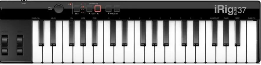
to MidiEditor, and Guitar Pro 5 (version 5.2), a program to create MIDI songs. The hardware that was being used for this experiment consisted of an IK Multimedia iRig Keys 37 MIDI controller keyboard (see Figure 2) and a HP notebook (model 15-ac120ND 15,6‘‘) which ran on Windows 10 Home 64-bit.

[image:10.595.70.527.184.423.2]

Figure 1. A screenshot of the program Synthesia in which participants had to press the corresponding key of the notes ‘falling from above’.

Figure 2. IK Multimedia iRig Keys 37 MIDI controller keyboard as used in this study.

Design

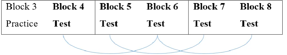
[image:10.595.79.521.495.605.2]

(11)

[image:11.595.72.526.457.519.2]

divided and assigned to one of these regimes. The first training regime, massed practice (MP), consisted of a single two-hour long session. The session was divided into eight blocks of ten minutes each with a five-minute rest between each block. The second training regime, distributed practice (DP), consisted of four 30-minute long sessions on four consecutive days (see Table 1). Each session for the distributed practice regime consisted of two blocks of ten minutes each with a five-minute rest between them. The contents of each block were the same for both conditions. The first three blocks were practice blocks and the last five blocks were the actual test blocks used for analysis. The experiment used a 2x5 mixed design with the dependent variables being correctly played notes, mistakes and duration accuracy, which will be explained later. The independent variables were the two practice regimes and the five test blocks.

Table 1

Overview of the blocks used in the experiment for the distributed practice group

Day 1 Day 2 Day 3 Day 4

Block 1 Block 2 Block 3 Block 4 Block 5 Block 6 Block 7 Block 8 Practice Practice Practice Test Test Test Test Test Note. All blocks were conducted on a single day for the massed practice group only.

Procedure

(12)

consent form was given to the participant. After agreeing with the informed consent and after it was signed, the experiment started.

The researcher asked the participant to click the button in Synthesia named ‘watch and listen only’ and told the participant to attentively listen to the song and see what the program looked like, while Synthesia played the song automatically. When the song was ended the researcher told the participant to begin with the first practice block. In these practice blocks the program waited for the participant to press the correct key, before continuing to the next notes of the song. The practice blocks were 10 minutes long and were repeated three times.

When the three practice blocks were finished, the experiment continued with the test blocks. In these test blocks the participant had to play along with the song at 60bpm. Now, the program did not wait for the correct input to continue, but the song was continued to be visually displayed. There was a total of five test blocks of 10 minutes each. In each test block the song was played seven times, which led to a total of 35 trials per participant.

After each block the researcher ended the recording, saved the file and started a new recording for the next block. Between each block was a short break in which the participant was informed to relax their fingers and their mind. The MP group completed all eight blocks (three practice blocks and five test blocks) in one session. The DP group completed two blocks per session per day, for four consecutive days. After the experiment was finished, the researcher thanked the participant and asked what the participant thought of the experiment. Finally, the researcher granted credits and/or a monetary compensation.

Analysis

(13)

[image:13.595.71.529.210.299.2]

total of 1400 trials (five blocks, seven trials per block for 40 participants). A trial was defined as a single, complete playthrough of the song Hallelujah. To establish differences between both groups, the trials were analysed on the before mentioned three dependent variables: correctly notes, mistakes and duration accuracy.All trials were saved as MIDI files.

Figure 3. Block comparison for the analysis.

Correctly played notes

The MIDI file of each participant was compared with the original song’s MIDI file in Rstudio. A note was marked as correct when the pitch of the note was correct, within an interval of 0.5 seconds of the target time in the score of the original note. If the correct note was accidentally played multiple times within the interval, only one note was marked as correct; the other note(s) as mistakes. The sum of the correct notes represented the dependent variable correctly played notes.

Mistakes

(14)

the original note, or if the timing exceeded the 0.5 second interval, the played note was marked as an error. The sum of the initial mistakes plus the error represented the dependent variable mistakes.

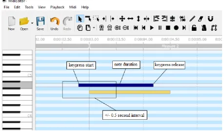
Duration accuracy

[image:14.595.68.528.352.620.2]

For the last component duration accuracy, the durations of the correct notes were compared with the durations of the corresponding original notes (see Figure 4). The absolute deviation was calculated only for the correctly played notes, in which a lower score indicated better duration accuracy.

(15)

Results

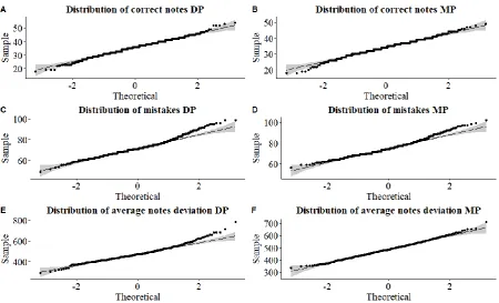
[image:15.595.73.524.184.457.2]

The data appeared to be normally distributed, as can be seen in the Q-Q plots below (see Figure 5), allowing parametric analyses.

Figure 5. Q-Q plots of the distribution of correct notes, mistakes and average notes deviation for the massed practice (MP) and distributed practice (DP) regimes.

Correctly played notes

(16)

[image:16.595.69.513.71.326.2]

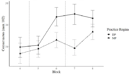
Figure 6. Line chart of correctly played notes per Block and per Practice Regime. The error bars represent one standard deviation. The vertical dashed lines represent the transitions from day 2 to day 3 and day 3 to day 4 for the distributed practice (DP) regime.

According to Mauchly’s test, the assumption of sphericity was violated p <.001. The degrees of freedom were corrected using Greenhouse-Geisser estimates of sphericity (ε = 0.67). Results show that the number of correctly played notes significantly changed over time; main effect of Block, F(2.69, 102.45) = 10.64, p <.01, ηp2 = 0.22. Both groups played more correct notes as

the experiment progressed (see Fig. 6).

The number of correctly played notes was also significantly affected by Practice Regime, F(1, 38) = 4.67, p =.04, ηp2 = 0.11. As hypothesized, participants with a distributed

practice regime played more correct notes compared to participants in the massed practice regime.

(17)

if (overnight) consolidation had occurred. The DP Regime played 2.8 correct notes more in Block 6 than in Block 4, p <.01, Cohen’s d =.532. The MP Regime did not have a significantly higher score between these blocks, p <.35, d =.24. For Blocks 5 and 7, the difference between the number of correct notes was 2.9 for the DP Regime, p <.01, d =.54. For the MP group there was no difference between these blocks, d = 0. Between Blocks 6 and 8 there was no significant difference found for both Practice Regimes (DP Regime, d =.02; MP Regime, d = .19).

Mistakes

[image:17.595.72.513.346.607.2]

The second part of the analysis concerned the mistakes that were made per Block for both Practice Regimes (see Figure 7).

Figure 7. Line chart of mistakes per Block and per Practice Regimes. The error bars represent one standard deviation.

(18)

A 2x5 mixed ANOVA was conducted with Practice Regime (between) and Block (within) as independent variables and mistakes as the dependent variable. According to Mauchly’s test, the assumption of sphericity was violated p <.01. The degrees of freedom were corrected using Greenhouse-Geisser estimates of sphericity (ε = 0.72). Results show that the number of mistakes significantly changed over time; main effect of Block, F(2.88, 109.29) = 21.32, p <.01, ηp2 = 0.36. Both Practice Regimes played fewer incorrect notes as the experiment

progressed.

The number of mistakes was also significantly affected by the Practice Regime, F(1, 38) = 7.53, p <.01, ηp2 = 0.10. As hypothesized, participants with a distributed practice regime

played fewer incorrect notes compared to participants in the massed practice regime.

There was no significant interaction between Block and Practice Regime, F(2.88, 109.29) = 1.86, p =.14, ηp2_{= 0.05. This indicates that overnight consolidation did not occur for} the variable mistakes.

Duration accuracy

The final part of the analysis consisted of the absolute note duration accuracy of correctly played notes, compared with the corresponding note duration from the original song file (see Figure 8). Again, a 2x5 mixed ANOVA was conducted with Practice Regime (between) and Block (within) as independent variables and duration accuracy as the dependent variable.

According to Mauchly’s test, the assumption of sphericity was not violated (p =.10), so no correction was needed. Results show that the length of note deviation significantly decreased over time; main effect of Block, F(4, 152) = 5.48, p <.01, ηp2 = 0.13. Both Practice Regime’s

(19)

There was no main effect for Practice Regime, F(1, 38) = 1.48, p =.23, ηp2 = 0.04.

Participants with a distributed practice regime did not have a significantly smaller deviation in absolute note duration than participants in the massed practice regime.

Finally, no significant interaction effect was found between Block and Practice Regime, F(4, 152) = 1.30, p =.27, ηp2 = 0.03. This again indicates that there was no effect of

consolidation for timing accuracy performance.

Figure 8. Line chart of timing accuracy per Block and per Practice Regime. The error bars represent one standard deviation.

[image:19.595.74.511.236.493.2]

(20)

Discussion

In the present study, the effect of massed versus distributed practice regimes was studied, with non-musicians who learned to play a song on a keyboard using piano training software. The massed practice regime consisted of a single two-hour long session, while the distributed practice regime was divided into four 30-minute long sessions across four consecutive days. It was expected that non-musicians who used a distributed practice regime would perform better on the number of correctly played notes, number of mistakes and duration accuracy, than their peers who used a massed practice regime. It was further hypothesized that consolidation would occur for the distributed practice group and that this effect would decrease after the first night of sleep (Simmons, 2012).

We found that when a distributed practice regime is applied, participants indeed perform better than when a massed practice regime is applied. The DP Regime played more notes correctly and made fewer mistakes. For duration accuracy there were no significant differences between the Practice Regimes, although a trend is visible in favour of the DP Regime (see Figure 8).

(21)

This study offers an exciting new method for teaching how to play a piano, for complete beginners who are not able to read sheet music. Furthermore, the implementation of the custom written script in the programming tool R (see Appendix B), based on the script written by Grasemann, R. (2018), enables researchers to analyse large amounts of MIDI data all at once, providing feedback in milliseconds, which was largely done before manually. It also makes it possible to analyse complete musical pieces at once, instead of breaking it down into small chunks. This new way of analysis not only saves time, it is also a safer and more consistent method for analysis and can be applicable in designing practice methods that suits the specific personal needs of an individual.

This study also confirms that sleep has a positive effect on performance for complete beginners. Therefore, it is recommended to apply a distributed practice regime for learning to play an instrument. This was examined with experienced learners only in most similar studies (Cash, 2009; Pike & Carter, 2010; Simmons & Duke, 2006; Simmons, 2012), and to the author’s knowledge not with non-musicians.

(22)

Informal conversations with the participants after the experiment revealed that it was difficult to play along with Synthesia on autoplay, and that they often lost track of keeping up the pace. Furthermore, some participants told that the task was very repetitive towards the end and this affected their focus and motivation. A possible solution to increase a participant’s intrinsic motivation is to add game elements in non-game context. This so-called gamification rewards the participant as they progress (Buckley, DeWille, Exton, Exton & Murray, 2018; Buckley & Doyle, 2016; Wagner, 2017). Even though Synthesia provides feedback on the performance of the player (for example the number of correctly played notes in a row), the appearance of the program is quite simplistic. When a more sophisticated interface is used, it might help to keep the participant focussed. Of course, this interface should not distract the participant from performing the actual task. As mentioned before, Hallam (1997) found that beginning musicians often do not play their practice material through entirely. For a follow up study, starting with short existing piano exercises which are developed for beginners, instead of immediately learning a whole song could be a solution to this issue.

Finally, for future studies it is recommended to increase the duration of the experiment. Participants in both groups did not seem to reach a ceiling across the blocks, so it is likely that continued improvements in performance would be observable when more sessions were held. According to Ericsson, Krampe and Tesch-Römer (1993), around 10,000 hours of deliberate practice are needed distributed across one decade, for mastering a skill like piano playing. This statement stands in sharp contrast with the two hours of practice in this study.

(23)

(24)

Literature

Abrahamse, E., Ruitenberg, M., de Kleine, E., & Verwey, W. (2013). Control of automated behavior: insights from the discrete sequence production task. Frontiers in human neuroscience, 7, 1-16.

Buckley, J., DeWille, T., Exton, C., Exton, G., & Murray, L. (2018). A gamification–motivation design framework for educational software developers. Journal of Educational Technology Systems, 47(1), 101-127.

Buckley, P., & Doyle, E. (2016). Gamification and student motivation. Interactive learning environments, 24(6), 1162-1175.

Cash, C. D. (2009). Effects of early and late rest intervals on performance and overnight consolidation of a keyboard sequence. Journal of research in music education, 57(3), 252-266.

Cohen, J. (1988). Statistical power analysis for the behavioral sciences (2nd ed.). Hillsdale, NJ: Lawrence Erlbaum Associates.

Ericsson, K.A., Krampe, R.T., & Tesch-Römer, C. (1993). The role of deliberate practice in the acquisition of expert performance. Psychological Review, 100, 363-406.

Grasemann, R. (2018). From chunking drills to Hallelujah: using new methods to train and evaluate complete piano beginners (Unpublished master's dissertation). University of Twente, Enschede, The Netherlands.

Gravetter, F. J., & Forzano, L. A. B. (2018). Research methods for the behavioral sciences (6th ed.). Belmont, CA: Wadsworth Cengage Learning.

Hallam, S. (1997). Approaches to instrumental music practice of experts and novices: Implications for education. Does practice make perfect, 89-107.

(25)

Hallam, S., Rinta, T., Varvarigou, M., Creech, A., Papageorgi, I., Gomes, T., & Lanipekun, J. (2012). The development of practising strategies in young people. Psychology of Music, 40(5), 652-680.

Kokotsaki, D., & Hallam, S. (2007). Higher education music students’ perceptions of the benefits of participative music making. Music Education Research, 9(1), 93-109. Kokotsaki, D., & Hallam, S. (2011). The perceived benefits of participative music making for

non-music university students: a comparison with music students. Music Education Research, 13(2), 149-172.

Palmer, C., & Meyer, R. K. (2000) Conceptual and motor learning in music performance. Psychological Science, 11(1), 63-68.

Pellegrino, K. (2011). Exploring the benefits of music-making as professional development for music teachers. Arts Education Policy Review, 112(2), 79-88.

Pike, P. D., & Carter, R. (2010). Employing cognitive chunking techniques to enhance sight- reading performance of undergraduate group-piano students. International Journal of Music Education, 28(3), 231-246.

Simmons, A. L., & Duke, R. A. (2006). Effects of sleep on performance of a keyboard melody. Journal of Research in Music Education, 54(3), 257-269.

Simmons, A. L. (2012). Distributed practice and procedural memory consolidation in musicians’ skill learning. Journal of Research in Music Education, 59(4), 357-368. Verwey, W. (1996). Buffer loading and chunking in sequential keypressing. Journal of

Experimental Psychology: Human Perception and Performance, 22(3), 544.

Verwey, W., Shea, C., & Wright, D. (2015) A cognitive framework for explaining serial processing and sequence execution strategies. Psychonomic Bulletin and Review, 22(1), 54–77.

(26)

(27)

(28)

Appendix B

R script for analysing the data

1. ## Process MIDI-files

2. library(signal)

3. library(tuneR)

4.

5. ## String editing

6. library(stringi)

7.

8. ## Tidy data

9. library(tidyverse)

10.

11.## Linear model

12.library(lmtest)

13.

14.##Levene's test

15.library(car)

16.

17.##Density plots##

18.library(ggpubr)

19.

20.##Side to side plots

21.library(cowplot)

22.

23.##Anova eta-squared package

24.library(ez)

25.

26.##Effect size computation

27.library(MOTE)

28.

29.install.packages('bindrcpp')

30.library(bindrcpp)

31.##

32.install.packages('dplyr')

33.library(dplyr)

34.

35.##Font type

36.

37.windowsFonts(Times=windowsFont("Times New Roman"))

38.

39.## Set working directory, may need adjustment on other computers

40.# Pay attention to maintaining the old folder structure

41.# or adjust code accordingly

42.setwd("C:/Users/…")

43.

44.## Do not execute if you want to read in new data

45.load("./.RData")

46.

47.### Data preparation ###

48.

49.## Create a list of all filenames as strings

50.filelist <- dir("Groups", pattern=NULL, all.files=FALSE, full.names=FALSE)

51.print(filelist)

52.

53.## Get data of original song

54.# convert GuitarPro-times to real time in millisecond

55.# round values to wholes

56.originalSong <- as.data.frame(getMidiNotes(readMidi(paste( "gp-hallelujah.mid")))) %>%

57. rename(tit = time) %>%

(29)

59. mutate(tit = round(tit * 2.083333)) %>%

60. mutate(length = round(length * 2.083333)) %>%

61. select(-track, -channel)

62.

63.## Data collection looping through all MIDI files

64.

65.## Get data of 1 participant and 1 trial

66.# convert Synthesia-times to real time in milliseconds

67.participantSong <- as.data.frame(getMidiNotes(readMidi(paste("./Groups/p1_120_4_1.mi d")))) %>%

69. mutate(tit = tit - tit[1]) %>%

70. mutate(tit = round((tit * 0.002717)*1000)) %>%

71. select(-track, -channel) %>%

72. mutate(Part = partNum) %>%

73. mutate(block = blockNum) %>%

74. mutate(trial = trialNum) %>%

75. mutate(Group = group)

76.

77.## Split filenames into meaningful bits

78.nameSplit <-

79. strsplit(filelist[1], "_") %>%

80. unlist()

81.## nameSplit[1] == partNum, [2] == group, [3] == blockNum, [4] == trialNum

82.# later on, rename group "120" to "MP" and group "4x30" to "DP"

83.print(nameSplit)

84.

85.## Create participant number

86.# here, we cut off the "p" from the participant's number in filename

87.partNum <-

88. stri_sub(nameSplit[1], 2)

89.print(partNum)

90.

91.## Create trial number

92.# here, we cut off the .mid from the trial number in filename

93.trialNum <-

94. stri_sub(nameSplit[4], from = 1, to = 1)

95.

96.## Create group indicator

97.# here, we transform a 120 to "MP" and a 4x30 to "DP"

98.if (nameSplit[2] == "120") {

99. group <- "MP"

100. } else {

101. group <- "DP"

102. }

103.

104. ## Create block number

105. blockNum <-

106. nameSplit[3]

107.

108. ### Now that we have all the pieces together, we can start building the loop ###

109.

110. ## Create a variable that serves as a handrail for the loop

111. loopcounter <- 0

112.

113. ## Create a list (of dataframes) that serves as a container for the loop's pr oducts

114. datalist = list()

115.

116. ## Start a for-loop that loops through our filelist from earlier

117. for (i in 1:length(filelist)) {

118. loopcounter <- loopcounter+1

119.

120. nameSplit <-

(30)

122. unlist()

123.

124. partNum <-

125. stri_sub(nameSplit[1], 2) %>%

126. as.numeric()

127.

128. blockNum <-

129. nameSplit[3]

130.

131. trialNum <-

132. stri_sub(nameSplit[4], from = 1, to = 1) %>%

133. as.numeric()

134.

135. if (blockNum == 5) {

136. trialNum <- trialNum + 7

137. } else if (blockNum == 6) {

139. } else if (blockNum == 7) {

141. } else if (blockNum == 8) {

143. } else {

144. trialNum <- trialNum

145. }

146.

147. if (nameSplit[2] == "120") {

148. group <- "MP"

149. } else {

150. group <- "DP"

151. partNum <- partNum + 21

152. }

153.

154. participantSong <- as.data.frame(getMidiNotes(

155. readMidi(paste("./Groups/",filelist[loopco unter], sep = "")))) %>%

157. mutate(tit = tit - tit[1]) %>%

158. mutate(tit = round((tit * 0.002717)*1000)) %>%

159. select(-track, -channel) %>%

161. mutate(block = blockNum) %>%

162. mutate(trial = trialNum) %>%

163. mutate(Group = group)

164.

165. ## Add the data just generated to our list (of dataframes)

166. datalist[[loopcounter]] <- participantSong

167. print(length(datalist))

168. print(paste("One down,",length(filelist)-loopcounter,"more to go."))

169. }

170.

171. ## Make an empty dataframe and add the dataframes from our list as new rows

172. allData <- data_frame() %>%

173. bind_rows(datalist) %>%

174. mutate(block = as.numeric(block)) %>%

175. mutate(trial = as.numeric(trial)) %>%

176. mutate(Part = factor(Part))

177.

178. ### Additional data transformation / Analysis ###

179.

180. ## Determine initial mistakes per participant, block, trial

181. # Make two dataframes for each group, we can collect total amount of mistakes there

182. levels(allData$Part)

183.

(31)

186.

187. # Iterate through all participants, make a list containg dataframes for each participant

188. for (i in levels(allData$Part)) {

189. partSlice <-

190. allData %>%

191. filter(Part == i)

192. print("partSlice successful!")

193. partList[[i]] <- partSlice

194.

195. print(paste("Participant number",partSlice$Part[1],"done."))

196. }

197.

198. # Empty list for initial mistakes

199. initMistList <- list()

200.

201. # Iterate through the list with participant-dataframes and compute initial mistakes per trial

202. for (j in 1:length(partList)) {

203. groupName <-

204. first(partList[[j]][[9]])

205.

206. partNum <-

207. first(partList[[j]][[6]])

208.

209. initMist <-

210. partList[[j]] %>%

211. group_by(trial) %>%

212. summarise(initMist = abs(length(tit) - 102), block = first(block)) %>%

214. mutate(Group = groupName)

215.

216. print("initMist assignment successful!")

217.

218. initMistList[[j]] <- initMist

219. print(paste(length(initMistList)))

220. }

221.

222. # Make dataframe from the list of initial mistakes per trial

223. allInitMist <- data_frame() %>%

224. bind_rows(initMistList) %>%

225. mutate(trial = as.numeric(trial))

226.

227. ## Make list for all trials

228. trialList <- list()

229.

230. for (j in 1:35) {

231. trialSlice <-

232. allData %>%

233. filter(trial == j)

234. print("trialSlice successful!")

235. trialList[[j]] <- trialSlice

236.

237. print(paste(trialSlice$trial[1],"done."))

238. }

239.

240. correctSliceList <- list()

241. correctSliceListTemp <- list()

242. correctRows <- data_frame()

243.

244. ## Loop through trialList, check for each row in originalSong if it exists in an element of trialList, delete all other rows and

245. # add results to list, also, we compute accuracy by computing how much each c orrectly played note deviated in sustain

(32)

247. for (j in 1:102) {

248.

249. interval <-

250. seq(originalSong$tit[j]-500,

251. originalSong$tit[j]+500,

252. by = 1)

253. print(paste(interval[1],interval[1001]))

254.

255. originalNote <-

256. originalSong$notename[j]

257. print(paste(originalNote))

258.

259. for (k in 1:35) {

260. correctSlice <-

261. trialList[[k]] %>%

262. filter(tit %in% interval) %>%

263. filter(notename == originalNote) %>%

264. mutate(accuracy = originalSong$length[j] - length) %>%

265. group_by(Part) %>%

266. filter(n() == 1) %>% ## Control for a doubly played correct note, if it happened, keep only one. We already controlled for this with initMist

267. ungroup()

268. correctSliceListTemp[[k]] <- correctSlice

269. print(paste("Checked trial",k,"of 35."))

270. }

271. correctSliceList[[j]] <- correctSliceListTemp

272. print(paste("Checked original note",j,"of 102."))

273. }

274.

275. ## Rejoin data we just separated into one dataset containing only correctly p layed notes

276. for (j in 1:102) {

277. for (k in 1:35) {

278. correctRows <-

279. bind_rows(correctRows, correctSliceList[[j]][[k]]) %>%

280. arrange(Part)

281. print(paste("Trial",k,"of note",j))

282. }

283. }

284.

285. ## Compute errors from correctly played notes and make list just like initMis t

286. mistList <- data_frame()

287.

288. for (k in 1:35) {

289.

290. mistList <-

291. bind_rows(mistList,

292. correctRows %>%

293. group_by(Part) %>%

294. filter(trial == k) %>%

295. summarise(mist = 102 - length(tit), accuracy = round(mean(accuracy))) %>%

296. mutate(trial = k)) %>%

297. ungroup() %>%

298. arrange(Part)

299. }

300.

301. ## Compute correctly played notes per trial and make list just like initMist

302. CorrNote <- data_frame()

303.

304. for (k in 1:35) {

305.

(33)

308. correctRows %>%

309. group_by(Part, Group, block) %>%

310. filter(trial == k) %>%

311. summarise(correct = length(tit), accuracy = round(mean(accura cy))) %>%

312. mutate(trial = k)) %>%

313. ungroup() %>%

314. arrange(Part)

315. }

316.

317. #

318.

319. ## Now we have two sets of mistake lists: mistList & allInitMist. Time to com bine them and have all mistakes

320. # of all participants in all trials

321. # pay attention that allInitMist and mistList have to be formatted in the sam e way (first by Part, then by trial)

322. # for this to work correctly

323. allMist <- allInitMist %>%

324. select(-Part, -trial) %>%

325. bind_cols(mistList) %>%

326. mutate(allMistakes = initMist + mist) %>%

327. select(-initMist, -mist)

328. ##

Q-Q plots of the distribution of both groups for correct, mistakes and accuracy

329.

330. qqplot1 <- ggqqplot(groupDP$correct, main = "Distribution of correct notes DP ") +

331. theme(plot.title = element_text(face = "bold", size=17, hjust = 0.5)) +

332. theme(text=element_text(size=17, family="serif"))

333.

334. qqplot2 <- ggqqplot(groupMP$correct, main = "Distribution of correct notes MP ") +

337.

338. qqplot3 <- ggqqplot(groupDP$allMistakes, main = "Distribution of mistakes DP"

) +

341.

342. qqplot4 <- ggqqplot(groupMP$allMistakes, main = "Distribution of mistakes MP"

) +

345.

346. qqplot5 <- ggqqplot(groupDP$accuracy, main = "Distribution of average notes d eviation DP") +

349.

350. qqplot6 <- ggqqplot(groupMP$accuracy, main = "Distribution of average notes d eviation MP") +

353.

354. plot_grid(qqplot1, qqplot2, qqplot3, qqplot4, qqplot5, qqplot6, labels="AUTO"

, ncol = 2, nrow = 3)

355.

356. cleanup = theme(panel.grid.major = element_blank(), 357. panel.grid.minor = element_blank(), 358. panel.background = element_blank(),

359. axis.line.x = element_line(color = "black"), 360. axis.line.y = element_line(color = "black"), 361. legend.key = element_rect(fill = "white"),

(34)

363. ## errorbar line graphs

364. Correctline = ggplot(CorrNote, aes(block, correct, linetype=Group, shape = Gr oup))

365. Correctline +

366. stat_summary(fun.y = mean,

367. geom = "point", size=3) +

369. geom = "line", size=1,

370. aes(group = Group)) +

371. stat_summary(fun.data = mean_cl_boot,

372. geom = "errorbar",

373. width = .2) +

374. xlab("Block") + ylab("Correct notes (max 102)") + labs(linetype = "Practice Regime") + labs(shape = "Practice Regime") + cleanup +

375. geom_vline(xintercept = 1.5, linetype = "dashed") +

378.

379. Mistakeline = ggplot(allMist, aes(block, allMistakes, linetype=Group, shape = Group))

380. Mistakeline +

388. width = .2) +

389. xlab("Block") + ylab("Mistakes") + labs(linetype = "Practice Regime") + labs(shape = "Practice Regime") +

390. cleanup +

394.

395. Accuracyline = ggplot(CorrNote, aes(block, accuracy, linetype=Group, shape = Group))

396. Accuracyline +

404. width = .2) +

405. xlab("Block") + ylab("Duration accuracy (ms)") + labs(linetype = "Practice Regime") + labs(shape = "Practice Regime") +

406. cleanup +

410. ##

411. ## Mixed anova (correct) with ezANOVA

412. CorrNote$block <- factor(CorrNote$block)

413. CorrNote$Group <- factor(CorrNote$Group)

414.

415. correctAnova <- ezANOVA(data = CorrNote,

416. dv = correct,

417. wid = Part,

418. within = block,

419. between = Group,

420. detailed = TRUE,

(35)

423. print(correctAnova)

424.

425. with(CorrNote, tapply(correct, list(block, Group), mean))

426. with(CorrNote, tapply(correct, list(block, Group), sd))

427. with(CorrNote, tapply(correct, list(block, Group), length))

428.

429. with(allMist, tapply(allMistakes, list(block, Group), mean))

430. with(allMist, tapply(allMistakes, list(block, Group), sd))

431. with(allMist, tapply(allMistakes, list(block, Group), length))

432. ## P value notation

433. options(scipen = 999)

434.

435. ## Mixed anova (mistakes) with ezANOVA

436. allMist$block <- factor(allMist$block)

437. allMist$Group <- factor(allMist$Group)

438.

439. mistakesAnova <- ezANOVA(data = allMist,

440. dv = allMistakes,

441. wid = Part,

445. type = 3

446. )

447. print(mistakesAnova)

448.

449. ## Mixed anova (accuracy) with ezANOVA

450. CorrNote$block <- factor(CorrNote$block)

451. CorrNote$Group <- factor(CorrNote$Group)

452.

453. accuracyAnova <- ezANOVA(data = CorrNote,

454. dv = accuracy,

455. wid = Part,

459. type = 3

460. )

461. print(accuracyAnova)

462.

463. ##

464. ## Post hoc test

465.

466.

467. pairwise.t.test(dataset$DV, dataset$IV,

468. paired = TRUE,

469. p.adjust.method = "bonferroni")

470.

471.

472. with(groupDP, pairwise.t.test(correct,

473. block,

474. paired = TRUE,

475. p.adjust.method = "bonferroni"))

476. with(groupMP, pairwise.t.test(correct,

477. block,

478. paired = TRUE,

480. with(groupDP, pairwise.t.test(allMistakes,

481. block,

482. paired = TRUE,

484. with(groupMP, pairwise.t.test(allMistakes,

485. block,

486. paired = TRUE,

(36)

489. pairwise.t.test(groupMP$correct, groupMP$block,

490. paired = TRUE,

491. p.adjust.method = "bonferroni")

492.

493. d.dep.t.avg(m1 = 70.5, m2 = 69.9,

494. sd1 = 6.55, sd2 = 5.98,

495. n = 140, a = .05)

496.

497. d.dep.t.avg(m1 = 33.8, m2 = 33.8,

498. sd1 = 4.56, sd2 = 4.32,

499. n = 140, a = .05)

500.

Learning to play music : Exploring massed versus distributed practice regimes for non musicians