ECE-205 Lab 6
Transfer Functions and an Optical Transmitter and Receiver
Overview
In this lab we will first learn how to implement transfer functions in both Matlab and in Simulink. Next we will build an optical transmitter and receiver. The transmitter/receiver is not related to the transfer functions, so don’t hurt yourself trying to figure out how the two parts of the lab are related. However, building the
transmitter and receiver will help with your circuit building skill and is pretty cool. You will need to get from me a photo transistor..
PART I: Representing Systems with Transfer Functions in Matlab and Simulink
Up until now we have represented our systems in terms of differential equations. In order to represent these systems in terms of transfer functions we only need to remember two simple things about Laplace transforms and transfer functions:
1) For transfer functions, we assume the initial conditions are zero (just as for the impulse response)
2) If
{ }
x t( ) =X s( ), then if we assume the initial conditions are zero we have dx t( ) sX s( )dt
=
and
2
2 2
( )
= s ( )
d x t
X s dt
3) The transfer function of a system is the transform of the output divided by the transform of the input.
You should be able to show that the transfer function for our first and second order system representations,
2 2
( ) ( ) ( )
( ) 2 n ( ) n ( ) = ( )n
y t y t Kx t
y t y t y t K x t
τ
ζω ω ω
+ = + + are 2 2 2 ( ) ( )
( ) 1 ( )
( )
( ) 2 n
n n
Y s K
H s
X s s
K Y s
H s
X s s s
τ ω ζω ω = = + = = + +
Next we need to learn to represent systems using transfer functions in both Matlab and Simulink Let’s first start with the way Matlab represents polynomials. If you wanted to represent the polynomial
2
( ) 3 2 1
p s = s + s+ in Matlab, you would enter the coefficients into an array p, p=[3 2 1]. The coefficients always go from high to low. The last (rightmost) entry in the array is the coefficient of s0 =1, or the constant term. You must also always include a number for every coefficient, even if that coefficient is zero. For example, to enter the polynomial 4
( ) 2 3
p s = s + sinto Matlab, you would type, p = [2 0 0 3 0].
For the most part, our transfer functions will be the ratio of two polynomials. We need to use the Matlab function tf, to tell Matlab that we want to construct a transfer function made up of two polynomials. For example, to enter the transfer function
num = [1 1]; % numerator polynomial of the transfer function den = [3 2 1]; % denominator polynomial of the transfer function H = tf(num,den); % construct the transfer function
We would, of course, just combine the three steps into one step,
H = tf([ 1 1],[3 2 1]);
If you do not put the semicolon at the end, Matlab will write the transfer function to the workspace (so you can check that you entered it correctly).
We will next show how to determine the response of a system represented by a transfer function to a step (or arbitrary input) in both Matlab and Matlab/Simulink. We will go through the steps for a first order system, then you will modify these for a second order system.
1) Open a new Matlab m-file (in a convenient folder). We will use one m-file for this lab. At the top of the file type the usual
clear variables
2) Set the variables tau = 0.001 and K = 2.0
3) Enter the transfer function
1 p
G K
s
τ =
+ into Matlab.
4) Enter the final time variable Tf = 0.01 (be sure to use at least one capitol letter so it is not confused with the transfer function command tf).
5) Use the linspace command to create a time vector t from 0 to Tf with 1000 sample points.
6) let’s assume we want a step input with an amplitude of 0.1. There are many ways to generate this, but we will use the following command:
x=0.1*ones(1,length(t));
7) To simulate the system, we then use the lsim command as follows:
y = lsim(Gp,x,t);
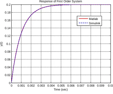
Figure 1. Response of first order system to a step of amplitude 0.1
We now want to prepare to use Simulink, and learn (and review) a few more commands as we go.
9) We will be using the times and input values from Matlab, so enter the command
ut = [ t’ x’]; % note that the apostrophe means take the transpose, leave a space between t’ and x’
into your m-file.
10) Athough we already know the numerator and the denominator of the transfer function, let’s learn to extract them once we have a transfer function. We use the command
[num_Gp,den_Gp] = tfdata(Gp,’v’);
to extract the numerator and denominator polynomials from the transfer function Gp.
11) Start Simulink from the Matlab window, and open a new model file. Save this model file as openloop.mdl.
12) Construct the model file shown in Figure 2. You will need to look in the Sources Library for the from workspace block and the clock block, the Sink Library for the to workspace blocks (be sure to save the data as an array, click on these boxes for this choice), and the Continuous Library for the transfer function block. Click on the transfer function block to enter the numerator as num_Gp and the denominator as den_Gp. Be sure to change the final time of the simulation to Tf. The final time of the simulation defaults to 10 seconds, and it appears in a box near the top of the Simulink model file.
0 0.001 0.002 0.003 0.004 0.005 0.006 0.007 0.008 0.009 0.01
0 0.02 0.04 0.06 0.08 0.1 0.12 0.14 0.16 0.18 0.2
Time (sec)
y
(t
)
Response of First Order System
Figure 2. The openloop Simulink file.
13) Run the simulation from the m-file using the command,
sim(‘openloop’);
14) At this point you have results from both Matlab (t,y) and Simulink (ts, ys). Modify your m-file to plot both of these results on the same graph. Use two different line types and colors, use a grid, label the x-axis etc. so your results look like that in Figure 1. You need to include your graph in your memo.
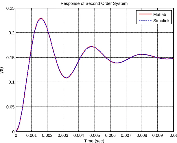
15) Now you need to modify your m-file so you can plot the results for a second order system with a natural frequency of 2000 rad/sec, a damping ratio of 0.2, and a static gain of 1.5. It is probably best to just copy and paste what you already have. If you have done everything correctly, you should get a graph like that shown in Figure 3. You need to include your graph in your memo, but not your code.
0 0.001 0.002 0.003 0.004 0.005 0.006 0.007 0.008 0.009 0.01 0
0.05 0.1 0.15 0.2 0.25
Time (sec)
y
(t
)
Response of Second Order System
Matlab Simulink
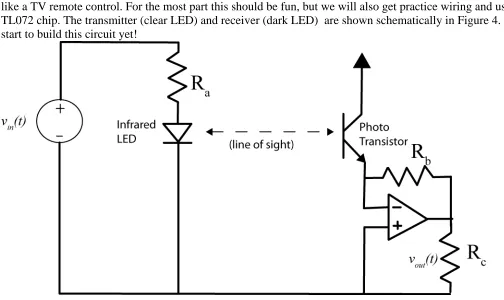
[image:4.612.149.455.473.720.2]PART II : Building an Optical Transmitter and Receiver
[image:5.612.35.539.92.392.2]In this part of the lab we will build a simple optical transmitter and receiver that utilizes infrared light, much like a TV remote control. For the most part this should be fun, but we will also get practice wiring and using a TL072 chip. The transmitter (clear LED) and receiver (dark LED) are shown schematically in Figure 4. Do not start to build this circuit yet!
Figure 4. General schematic of optical transmitter and receiver.
The transmitter, on the left of the diagram, consists of an infrared LED. You will not be able to see when this is on, though you may be able to see it if you have a camera on your cell phone and look through that. The right side of the diagram shows the receiver, which consists primarily of a photo transistor and an amplifier. There are some tricks to building this circuit which we expect you to use later in this course.
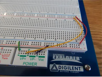
1) The first thing we want to do is set the ground and the two power rails, just as we did for lab 4. First connect one of the grounds (a down arrow) to the blue “rail” and then use another wire to connect the top and bottom blue rails together. It is better to do this somewhere away from the board where the USB and power connectors are. Next connect a wire from VP+ to the top red rail (this will be our VCC) and connect a wire from VP- to the bottom red rail (this will be our −VCC). Both VCC and −VCC are just to provide the necessary voltages to our trop amp, they are not the input signals. Figure 5 shows how I connected these. Note that we want as much room on our breadboard as possible for the transmitter and receiver .
Figure 5. Connect the power at the end of the board so they do not interfere with the transmitter or receiver.
Figure 6 shows my final wiring for this circuit. The important part of this is that we are trying to separate the transmitter and the receiver. Do not put these right next to each other!
Figure 7 shows a more detailed wiring diagram for building this circuit. You should lay out your breadboard in this fashion, with the LED and phototransistor straddling the centerline.
3) First we will build the transmitter on the left of Figure 7. Use the infrared LED (the clear LED) and connect it to the function generator through the Ra =51Ω resister. Be sure the function generator and the output of the LED are connected to ground. Try and build this as far to the left end of your circuit board as possible. Finally, connect DC1 to measure the voltage across the LED relative to ground.
[image:7.612.38.572.257.582.2]4) Next we will build the receiver, which should be built as far to the right as possible. Note that we are using anTL072 chip which includes two op amps on one chip. Be sure to dot on the chip is to the left (the semicircle on the drawing) and also to connect the power supplies correctly for this chip (they are different than for a 741 op amp!). Also be sure to connect the positive pin of the first op amp (the one we are using) to ground. Connect the rest of the circuit, usingRb =10 kΩ and Rc= Ω1k . Finally, the output of the receiver circuit is the voltage across the output resister Rc, so connect DC2 as shown in Figure 7.
Figure 7. More detailed schematic of the optical transmitter and receiver.
5) The transmitter is at the end of the LED, and the receiver is at the end of the phototransister, so you need to bend these at a 90 degree angle so they are pointing towards each other at this point. You will probably have to modify the pointing once we start to measure the received signal.
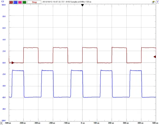
7) Set the Oscilloscope to measure 1 Volt/Div for both channels The Time/div should be set initially to100
sec
[image:8.612.38.575.178.598.2]µ . Turn on the power to the positive (VCC) and negative ( -VCC) voltage rails. Start the oscilloscope, and you should see something like that in Figure 8. Note that at this point you may need to modify the transmitter and receiver so they are pointing more accurately. You may also need to shield your system from ambient light by putting a few pieces of paper over the top of it. The LED is transmitting when the voltage across it is high, and the phototransister is receiving when the voltage across the output/load resistor is low. Capture your picture and put it in your memo and you are done!