ISSN Online: 2327-5227 ISSN Print: 2327-5219
DOI: 10.4236/jcc.2018.69007 Sep. 20, 2018 73 Journal of Computer and Communications
Fuzzy Mathematical Model for Solving Supply
Chain Problem
Yi-Shian Chin
1, Hsin-Vonn Seow
1*, Lai Soon Lee
2,3, Rajprasad Kumar Rajkumar
41Nottingham University Business School, University of Nottingham Malaysia Campus, Semenyih, Malaysia
2Laboratory Computational Statistics and Operations Research, Institute for Mathematical Research, University Putra Malaysia, Serdang, Malaysia
3Department of Mathematics, Faculty of Science, University Putra Malaysia, Serdang, Malaysia
4Department of Mechanical, Materials and Manufacturing Engineering, Faculty of Engineering, University of Nottingham Malaysia Campus, Semenyih, Malaysia
Abstract
In a real world application supply chain, there are many elements of uncer-tainty such as supplier performance, market demands, product price, opera-tion time, and shipping method which increases the difficulty for manufac-turers to quickly respond in order to fulfil the customer requirements. In this paper, the authors developed a fuzzy mathematical model to integrate differ-ent operational functions with the aim to provide satisfy decisions to help de-cision maker resolve production problem for all functions simultaneously. A triangular fuzzy number or possibilistic distribution represents all the uncer-tainty parameters. A comparison between a fuzzy model, a possibilistic model and a deterministic model is presented in this paper in order to distinguish the effectiveness of model in dealing the uncertain nature of supply chain. The proposed models performance is evaluated based on the operational as-pect and computational asas-pect. The fuzzy model and the possibilistic model are expected to be more preferable to respond to the dynamic changes of the supply change network compared to the deterministic model. The developed fuzzy model seems to be more flexible in undertaking the lack of information or imprecise data of a variable in real situation whereas possibilistic model is more practical in solving an existing systems problem that has available data provided.
Keywords
Supply Chain, Fuzzy Model, Possibilistic Model, Undertainty, Triangular Fuzzy Number
How to cite this paper: Chin, Y.-S., Seow, H.-V., Lee, L.S. and Rajkumar, R.K. (2018) Fuzzy Mathematical Model for Solving Supply Chain Problem. Journal of Com-puter and Communications, 6, 73-105.
https://doi.org/10.4236/jcc.2018.69007
Received: July 31, 2018 Accepted: September 17, 2018 Published: September 20, 2018
Copyright © 2018 by authors and Scientific Research Publishing Inc. This work is licensed under the Creative Commons Attribution International License (CC BY 4.0).
DOI: 10.4236/jcc.2018.69007 74 Journal of Computer and Communications
1. Introduction
In today’s global marketplace, individual enterprise is no longer sought after for individual achievement. In order to secure their business under rigorous market pressure and challenges for a long-term perspective, they tend to integrate themselves as part of the supply chain to propel their business. As the internet and information technology grow rapidly, the flow of information among dif-ferent functions is the main key to drive supply chain performance. [1] shares the five main supply chain practices that will equip a business to stay competi-tive and improve its organizational performance. These are supplier partnership, customer relationship, quality of information sharing, level of information shar-ing and postponement. In other words, the truly integrated and strong relation-ship formed among supply chain members is an essential prerequisite to succeed in the global market.
The attention on the development of the concept for supply chain manage-ment has gradually drawn the attention from academicians, business/industry managers, and consultants. The concept has been evaluated, practiced, examined and proven to be able to address various supply chain issues and influence the firm’s performance [1] [2] [3]. A supply chain model plays a significant role in supply chain management (SCM) for reducing the operational costs, reducing cycle time, and improving order-fulfilment rate and customer satisfaction level. This approach is proven and verified to be able to increase supply chain effi-ciency and delivers extra value to customers.
A supply chain (SC) is a dynamic network that consists of a high degree of uncertainty that generates from the flow of material and information, and passes through different operational functions in order to deliver goods to the end user. In general, a whole supply chain is triggered by demands from downstream sites (customers) and upstream sites (procurement, production, and distribution) which are cooperating and coordinating to transform raw materials into finished products and deliver it to customers [4]. The problem of this study is to consider a supply chain that consists of all functions and the need to meet the customers’ demand on time; with possible uncertainties occurring from all parties in the supply chain network. Much research has been carried out work to address the supply chain problem by contemplating different operational functions rather than to integrate all functions due to the complexity of a supply chain. Thus, there is little work on an integrated manner to solving the resources’ planning in this supply chain problem.
loca-DOI: 10.4236/jcc.2018.69007 75 Journal of Computer and Communications tion-allocation problem, plant sizing, product selection, capacity expansion and distribution channel design [7]. A tactical model is considered as a mid-term planning model and mostly applied in optimizing SC process performance by utilizing available resources such as supplier, inventory, distribution center and transportation. This mid-term model is use for one to two years planning efforts. An operational model is characterized as a short-term planning model and fo-cuses on schedule details such as lot size, day-to-day processing variations, can-cellation or top up orders, vehicle route, and an assigned load [5]. In this study, a tactical model will be designed and developed for the supply chain planning problems dealing with uncertainty which has not been researched much upon.
2. Literature Review
In the 90s and before the fuzzy set theory was introduced, operation manage-ment was leaning towards reducing the complex real world problems with attributes of precise mathematical modeling and this approach became one of the most important fields in science and engineering at that time. However, re-searchers realized that a precise mathematical model is not achievable under “real-world” supply chain situations. Thus, they started to employ the concept and techniques of probability theory to deal with this real-world uncertainty sit-uation. Fuzzy set theory which was first introduced by [8] started being used to define the imprecision of data based on degree of fitness rather than random va-riables [9].
In Operations Research, fuzzy set theory has been applied techniques of linear and nonlinear programming, dynamic programming, production resource plan-ning, queueing theory, multi-objective decision-making, to name a few applica-tions [2] [9]. In 1978, [10] presented another theory that relates to the fuzzy sets and named it as Possibilistic Theory. He demonstrated under “information pro-vided” situation, most of the decision-making is based on the possibilistic nature rather than probability. [11] explained that probability describes whether the event occurs and to what degree of it occurs is fuzzy. Fuzzy set theory is a theory of graded concept (degree of a matter) and is not focused on a chance the event will occur; this is the difference between concept randomness and fuzziness [9]. Possibilistic Theory explains how likely of the event may happen. Possibility theory is treats as alternative of probability theory to deal with the uncertain sit-uation. This shows that the probability model has its limitations in modelling all possible problems of incompleteness.
Fuzzy modeling approach is widely used in solving the problems in aggregate planning, manufacturing resource planning, transportation planning, inventory management, and supply chain planning [12]. The fuzzy set theory has been ap-plied to different problems related to the supply chain planning, such as the fol-lowing:
1) Aggregate planning
produc-DOI: 10.4236/jcc.2018.69007 76 Journal of Computer and Communications tion planning (APP) problem which identify demand and process uncertainty. Trapezoidal fuzzy number is used to present the fuzzy parameters in the model. They state that traditional linear programming is not the best choice for pre-dicting medium and long-term planning horizon due to the fluctuation of mar-ket demands and inconsistency of production parameters in real situation. They proposed a fuzzy linear programming approach that is more adequate and rea-listic approach to use for solving the production planning problem through con-tinuous modeling problem according to the available information.
2) Manufacturing resource planning
[14] compared the traditional LP with deterministic coefficient with a fuzzy linear programming model in determining the production-planning schedule for fresh tomato packing in Ruskin, Florida. This study showed the fuzzy linear programming approach is more practical and characterized the real-life toma-to-packing situation by relaxing some resource restriction. Results showed that the average operation cost using the fuzzy modeling method is 10 times less than traditional linear programming and the service satisfaction level increased as well. [15] used possibilistic theory combined with [16]’s fuzzy programming method to obtain a compromise solution to minimize the production operation cost and decision satisfactory information. This approach was implemented in production for resource planning in dealing with assemble-to-order environ-ment under demand uncertainty situation. The solution helped in determining the safety stock level and to decide the number of key machined used for reduc-ing the capital waste. This paper results showed that this approach was compe-tent in the decision making process when dealing with imprecise data. [17] ap-plied a similar approach as [15] in solving a real industry aggregate production planning (APP) problem in their research to help determine the 18-month pro-duction resource-planning. The solution could be improved through iteratively modifying the possibilistic distirbution. [17] demonstrated that a compromise solution for APP can be obtained with the overall satisfaction result guidance in the modelling process.
3) SC inventory management
[18] aimed at integrating the SC model with simulation control to determine the inventory’s stock level and order quantity in a finite time horizon, to minim-ize the supply chain cost, with an acceptable delivery performance. The uncer-tainties considered in the fuzzy model are external supplier late delivery and fluctuation of customer demand. The SC model was developed to deal for the uncertainty elements and determine the inventory’s order-up-to stock level; whereas the SC simulator was used to evaluate the decision made by the SC fuzzy model. [19] extends his research work with a proposed simulation tool named SCSIM to do analysis and evaluate the dynamic behavior of a series of supply chain under uncertain environment to enhance the decision making.
4) Transportation planning
DOI: 10.4236/jcc.2018.69007 77 Journal of Computer and Communications supply chain cost through identifying the allocation of orders to depots, ar-rangement of sending and returning of vehicles to depots. This model is built with consideration with multiple depots, multiple vehicles, multiple products, multiple customers and with different periods. A two-ranking function is used to solve planning problems and a regression model is developed to analyze the ap-plied fuzzy ranking method. Results expressed the flexibility of fuzzy modeling in representing a real life environment.
[21] optimized the supply chain procurement transportation operational planning (SCPTOP) problem using fuzzy multi-objective integer linear pro-gramming model (FMOLP). This solution in a real automobile industry sector with integration with the automobile assembler, a first tier supplier and second-tier supplier was used in solving the procurement and transporta-tion-planning problem simultaneously. This study helps decision-makers con-vert the manual decision procedure into an automatic mode, which provides a better result in controlling their total stock level, and benefits each supply chain party.
5) Supply chain planning
trapezoid-DOI: 10.4236/jcc.2018.69007 78 Journal of Computer and Communications al fuzzy number. More recently, [26] reported an investigation regarding the benefit of using fuzzy set theory to model and solve supply chain problems in the manufacturing industry. This model has been tested with the real data obtained from a real-world automobile supply chain by using CPLEX software. The re-search result expresses that fuzzy modeling is clearly superior to deterministic model in handling the real situations especially when there are pre-existing im-precise information. [27] extends this research, which includes a supply chain global satisfaction degree by considering the aspect of service level, inventory cost, planning nervousness (period and quantity) and overall cost. [28] revealed that the design of a supply chain has more advantages when dealing with supply uncertainty for a multi-stage and multi-echelon supply chain network. They ex-pressed that supply chain centralization is always a suitable strategy under high or low risk supply uncertainty and it able to fulfill market demand with lowest price.
[29] proposed to apply the possibilistic approach in solving the water quality management planning problem and this solution help in solving economic and environmental factor simultaneously. An inexact agricultural water quality man-agement (IAWQM) model is developed to consider the agricultural activities can be generated under restriction of water quality and quantity variable in order to maximize the agricultural income. The result provided a schematic decision in identify the cropping area, fertilizer applied and livestock husbandry size, in-corporating water management knowledge. [30] extended [15] research work by applying a similar possibilistic approach into the supply chain modelling to solve for multi-product and multi-period manufacturing and distribution planning decision (MDPD) in the real SC situation. In this research, the effectiveness of a possibilistic model and deterministic model is compare in solving the SC plan-ning problem under the uncertainty. Research result presets that the proposed possibilistic model solution is more efficient and practical when practiced in the real world MDPD. [31] proposed a possibilistic linear programming model to solve for supply chain problems in the bus-manufacturing company. 11 experi-ments have been designed, with a sensitivity analysis test to validate the consis-tency of the model. The solution was able to provide the manager with informa-tion and guidance in preparing their strategy for in-house resources planning.
DOI: 10.4236/jcc.2018.69007 79 Journal of Computer and Communications of imprecise data, lack of information or a new design product forecast for those uncertainties parameters in the model. This study proposes a multi-stage, single product, multi-echelon and multi-period supply chain network to investigate the benefit of the fuzzy linear programming (FLP) model and possibilistic linear programming (PLP) in dealing with demand uncertainty, process uncertainty and supply uncertainty issues.
This study focuses on optimizing the supply chain resources’ planning under demand, supply and process uncertainties with using mixed-integer linear pro-gramming method. A fuzzy mathematic model is developed integrating different functions of the supply chain with target to minimize the operational cost using an optimal planning solution. The objectives of this study are:
1) To model a supply chain problem that deals with procurement, production, and distribution planning under uncertainty.
2) To develop a mathematic model to include uncertainties from supplier, process and demand, where these parameters are represented by a triangular fuzzy number.
3) To provide solutions to resolve decision-making problems for different op-erational functions simultaneously with a developed model.
4) To investigate the benefits and effectiveness of fuzzy set theory in FLP and PLP in modeling and solving supply chain problem.
3. Case Description
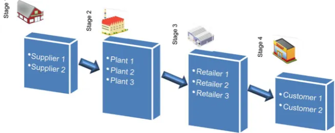
This study describes the multi-stage, multi-echelon, multi-time period, single product and single objective fuzzy possibilistic model which incorporates three types of uncertainty. The types of uncertainty involved in this model are demand uncertainty, process uncertainty and supplier uncertainty. This supply chain system consists of four echelons which are supplier, production plant, distribu-tion and customer as shown in Figure 1.
This model is assumes a single product is manufactured at one time period, and each product is made by two types of raw material. The objective of a fuzzy linear programming approach is proposed in this paper is aimed to minimize operation cost while providing a systematic framework which is able to integrate all fuzzy variables in the supply chain model under uncertainty. This approach is also considers the decision makers’ satisfaction and enable them adjust the fuzzy parameters in order to obtain a satisfy solution.
The following are the assumptions made for modelling the supply chain model:
1) Each customer order is independent. Backorder demand is considered in this supply chain and backorder demand must be fulfilled in the next time pe-riod.
2) All demands must be fulfilled at the end of the planning horizon and no backorder demand is allowed in the end of planning horizon.
DOI: 10.4236/jcc.2018.69007 80 Journal of Computer and Communications Figure 1. Supply chain link: research region.
4) All the fuzzy parameters are represented using a triangular membership function.
5) No safety stock is considered in the production plant and distribution cen-ter’s inventory.
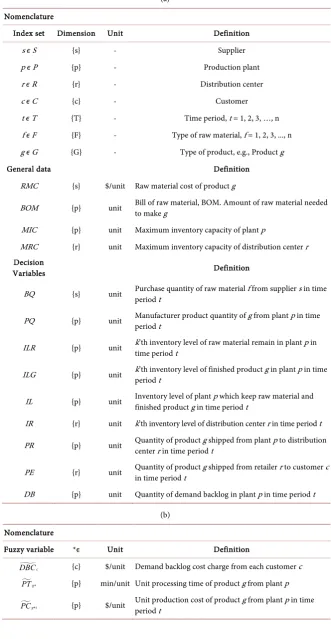
Many parameters are introduced in this supply chain model which includes general data, decision variables and fuzzy variables. In this formulation, a wav-ing symbol (~) is used to represent a fuzzy variable. Dimension explains the
echelons [supplier(s), plant (p), distribution center(r) and customer(c)] involved for each variables in the mathematic model (Table 1).
3.1. Fuzzy and Fuzzy Possibilistic Linear Programming Model
3.1.1. Objective Function
In this study, the proposed linear programming objective is to minimize the overall operation cost though optimized arrangement of the operation resources. The cost coefficients consider in multi-stage, multi-echelon and multi-time pe-riod model are raw material cost, production cost, inventory cost, transportation cost and demand backlog cost. The following is the fuzzy objective function for minimize the operation cost:
minimize raw material cost production cost
plant s inventory cost Distribution center s inventory cost transportation cost Demand backlog cost
z= +
+ +
+ +
∑
∑
∑
∑
∑
∑
’ ’
0 0 0 0 0 0
0 0 0 0 0 0
0 0 0 0 0 0 0 0
min fs fst gpt gpt
t s f t p g
pt
fpt grt grt
t p f t r g
gprt
fpst fpst gprt
t s p f t p r g
c
T S F T P G
T P F T R G
T S P F T P R G
grt cgrt
g
z RMC BQ PC PQ
ILR IC IR HC
TC BQ TC PR
TC PE
= = = = = =
= = = = = =
= = = = = = = =
= ⋅ ⋅ + ⋅
⋅
+ +
+ +
+
⋅
⋅ ⋅
⋅
∑∑ ∑
∑∑ ∑
∑∑ ∑
∑∑∑
∑∑∑ ∑
∑∑∑∑
0 0 0 0 0 0 0 gct ct
t r t g
T R C G
c
G T C
c= DB DBC
= = = = = =
+ ⋅
∑∑∑∑
∑∑∑
(1)
1) The total raw material cost:
DOI: 10.4236/jcc.2018.69007 81 Journal of Computer and Communications Table 1. Nomenclature for supply chain model.
(a) Nomenclature
Index set Dimension Unit Definition
s є S {s} - Supplier
p є P {p} - Production plant
r є R {r} - Distribution center
c ϵ C {c} - Customer
t ϵ T {T} - Time period, t = 1, 2, 3, …, n
f ϵ F {F} - Type of raw material, f = 1, 2, 3, ..., n
g ϵ G {G} - Type of product, e.g., Product g
General data Definition
RMC {s} $/unit Raw material cost of product g
BOM {p} unit Bill of raw material, BOM. Amount of raw material needed to make g
MIC {p} unit Maximum inventory capacity of plant p
MRC {r} unit Maximum inventory capacity of distribution center r
Decision
Variables Definition
BQ {s} unit Purchase quantity of raw material f from supplier s in time period t
PQ {p} unit Manufacturer product quantity of g from plant p in time period t
ILR {p} unit k’th inventory level of raw material remain in plant p in time period t
ILG {p} unit k’th inventory level of finished product g in plant p in time period t
IL {p} unit Inventory level of plant p which keep raw material and finished product g in time period t
IR {r} unit k’th inventory level of distribution center r in time period t
PR {p} unit Quantity of product g shipped from plant p to distribution center r in time period t
PE {r} unit Quantity of product g shipped from retailer r to customer c in time period t
DB {p} unit Quantity of demand backlog in plant p in time period t
(b) Nomenclature
Fuzzy variable *ϵ Unit Definition
c
DBC {c} $/unit Demand backlog cost charge from each customer c
g
PT∗ {p} min/unit Unit processing time of product g from plant p
g t
PC∗ {p} $/unit Unit production cost of product g from plant p in time
DOI: 10.4236/jcc.2018.69007 82 Journal of Computer and Communications Continued
fg t
IC ∗ {p} $/unit Unit inventory holding cost of plant p in time period t
g t
HC∗ {r} $/unit Unit inventory holding cost of distribution center r in time
period t
t
TC∗ {s, p, r} $/unit Unit transportation cost for each part of raw material f or product g in time period t
f
MBC∗ {s} unit Maximum procurement capacity of raw material f for
supplier s
gt
D∗ {c} unit
Demand request for product g from customer c in time period t
g
MPC ∗ {p} unit Maximum production capacity of plan p
g
MTC∗ {p, r} unit Maximum output transportation capacity for product g
from plant p to retailer r or from retailer r to customer c
brought into production plant is the total raw material cost on period t.
0 0 0
T S F
fs fst
t s f
RMC BQ
= = =
⋅
∑∑ ∑
(2)2) The total production cost:
Total amount of product, g manufactured in plant p multiplied by the unit product cost is equal to the production cost on period t.
0 0 0
T P G
gpt gpt
t p p
PC PQ
= = =
⋅
∑ ∑ ∑
(3)3) The total inventory cost: a) Plant’s inventory cost:
This model assumes that each plant p has its own inventory for storing the finished goods and remaining raw material left from the previous period t. However, this inventory has its capacity and inventory holding will be charged. Inventory in the production plant p includes raw material and finished goods.
Plant Inventory cost
Raw material inventory cost Finished product inventory cost
= +
∑
∑
∑
For the inventory level of raw material f at the plant, p in time period t, the balance equation can be written as follow:
Inventory in the end of the period t = inventory level of period t − 1 + re-ceived raw material f shipment from supplier s in time period t –total material used for manufacture product g in time period t.
So for time period t =1:
0 0 0 , , ,
S G G
fpt fpst fg gpt
s g g
ILR BQ BOM PQ f p t
= = =
= − ⋅ ∀
∑
∑
∑
For time period t > 1:
( )1
0 0 0 , , ,
S G G
fpt fp t fpst fg gpt
s g g
ILR ILR − BQ BOM PQ f p t
= = =
= + − ⋅ ∀
DOI: 10.4236/jcc.2018.69007 83 Journal of Computer and Communications For the inventory level of finished product g at the plant p in time period t, the balance equation can be written as follows:
Inventory in the end of the period t =inventory level of period t − 1+total manufacturer product g manufactured in plant p in time period t −total quanti-tyof finished product g deliver from plant p to distribution center r in time pe-riod t.
For time period t = 1:
0 , , ,
R
gpt gpt gprt
r
ILG PQ PR g p t
=
= −
∑
∀For time period t > 1:
( )1
0
, , ,
R
gpt gp t gpt gprt
r
ILG ILG − PQ PR g p t
=
= + −
∑
∀ (5)Thus, the summation of the inventory cost in plant p in time period t can be written as follow:
0 0 0 0 0 0
Plant inventory cost
Raw material inventory cost finished product inventory cost
T P F T P G
pt pt
fpt gpt
t p f t p g
ILR IC ILG IC
= = = = = =
= +
= ⋅ + ⋅
∑
∑
∑
∑ ∑∑
∑ ∑ ∑
(6)
b) Distribution center’s inventory cost:
Distribution center r also has its inventory space to keep the finished product,
g before shipping to customer c in time period t.The balance equation can be written as follows:
Inventory in the end of the period t = inventory level of period t − 1 + receive finish product g from plant p in time period t − total quantity of product g de-liver to customer c from distribution center r in time period t.
For time period t = 1:
0 0
, , ,
P C
grt grpt cgrt
p c
IR PR PE g r t
= =
=
∑
−∑
∀For time period t > 1:
( )1
0 0 , , ,
P C
grt gr t gprt cgrt
p c
IR IR − PR PE g r t
= =
= +
∑
−∑
∀ (7)Thus, the sum of the distribution center’s (DC) inventory cost consumption can be written as follow:
0 0 0
Distribution center inventory cost
DC sinventory level inventory holding cost
T R G
grt grt
t r g
IR HC
= = =
= ⋅
= ⋅
∑
∑
∑∑∑
’
(8)
4) The total transportation cost:
Total transportation cost is divide into 3 stages, it includes:
DOI: 10.4236/jcc.2018.69007 84 Journal of Computer and Communications
p in time period t;
b) shipment cost to delivery product from plant, p to distribution center, r in time period t;
c) shipment cost for ready stock delivery from distribution center, r to cus-tomer, c site in time period t.
The balance equation can be written as follow:
Transportation cost in the end of the period t = shipping cost for deliver raw material f from suppliers to plant p in time period t + deliver the finish product
g from plant p to distribution center in time period t + total quantity of product
g deliver to customer c from distribution center r in time period t. Transportation cost
Trans. supplier_plant Trans. plant_DC Trans DC_cust
= + +
∑
∑
∑
∑
The total transport cost from supplier, s to production plant, p for raw ma-terial, f shipment in time period t:
0 0 0 0
T P R G
fpst fpst
t= p= r= g=TC BQ
⋅
∑ ∑∑∑
(9)The total transport cost from production plant, p to distribution center, r for product, g shipment in time period t:
0 0 0 0
T P R G
gprt gprt
t= p= r= g=TC PR
⋅
∑ ∑∑∑
(10)The total transport cost from distribution center, r to customer, c for product,
g shipment in time period t:
0 0 0 0
C
T R G
cgrt cgrt
t r c g
TC PE
= = = =
⋅
∑∑∑∑
(11)5) Demand backlog cost:
If output of production plant is unable to meet the demand target as per cus-tomer request, the shortage unit is considered as demand backlog and penalty will be charge for the delay in shipment. The balance equation of demand back-log on period t can be written as follow:
Demand backlog of the period t = demand backlog level of period t − 1 + de-mand request by customer c in time period t − total quantity of product g deliver to customer c from distribution center r in time period t.
For time period t = 1:
0 , , ,
R
gct cgt cgrt
r
DB D PE g c t
=
= −
∑
∀For time period t > 1:
( )1
0 , , ,
R
gct gc t cgt cgrt
r
DB DB − D PE g c t
=
= + −
∑
∀ (12)DOI: 10.4236/jcc.2018.69007 85 Journal of Computer and Communications
0 0 0
C
T G
ct gct
t g c
DB DBC
= = =
⋅
∑∑∑
(13)3.1.2. Constraints
1) Supplier constraint
The total amount of purchase raw material f from each supplier, s should not greater than maximum procurement capacity.
sf, , ,
sft
BQ ≤MBC ∀s f t (14) 2) Demand constraint
Assumes that the total amount of product g shipped from distribution center,
r to each customer, c is referred as customer demand. The amount of product deliver to customer c is as per order requested.
0
0 , , ,
R
cgt cgrt
r
D = PE c g t
=
=
∑
∀ (15)
3) Inventory constraint
Inventory stock level for raw material, f and finish product, g in plant, p can-not exceed the maximum inventory capacity level in time period t. Distribution center’s inventory also applies the same rule.
a) Plant’s inventory constraint
Let IL be defined as the plant’s inventory level which use for stores the raw material, f and finished product, g in time period t.
0 0
, ,
F G
pt fpt gpt
f g
IL ILR ILG p t
= =
=
∑
+∑
∀ (16)The plant inventory level, IL is controlled not to exceed the plant’s maximum inventory capacity in time period t.
, ,
pt P
IL ≤MIC ∀p t (17)
b) Retailer’s inventory constraint:
The distribution inventory level, IR is controlled not to exceed the distribution center’s, r maximum inventory capacity in time period t.
, , ,
grt gr
IR ≤MRC ∀g r t (18)
4) Production constraint
The quantity of product, g manufactured in plant, p is controlled to not to ex-ceed the maximum production capacity.
gp gp, , ,
gpt
PQ ⋅PT ≤MPC ∀g p t (19)
5) Transportation constraint
The product, g ships out quantity from plant, p to distribution center, r
should not exceed the limit of transportation capacity. It applies the same rule for the transportation from distribution center, r to customer zone, c.
gpr, , , ,
gprt
PQ ≤MTC ∀g p r t (20)
grc, , , ,
grct
DOI: 10.4236/jcc.2018.69007 86 Journal of Computer and Communications 6) Demand backlog constraint
The total of finished product g shipped to customer c is always less than the total amount of demand on time t plus the demand backlog of previous period, t
− 1.
1 , , ,
cgt gt cgt
PE ≤DB − +D ∀c g t (22)
3.2. Strategy to Convert Fuzzy Objective into Equivalent Auxiliary
Crisp Linear Programming for FLP Model
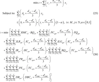
In order to transform the fuzzy mixed integer linear programming (FMILP) into an equivalent auxiliary crisp MILP model a special treatment need to be perform for those uncertainty parameter in the model. The uncertainty elements in this model are supplier, process operation and demand. These uncertainties are la-belled as fuzzy coefficients existing in the objective function and constraint in the model. In order to address the uncertainty parameters for FMILP, the ap-proach of representation theorem and technological coefficient proposed by [32] is applied in this study.
The transformation from fuzzy mixed integer linear programming (FMILP) to auxiliary a parametric integer linear programming is written as following:
Objective function:
maxcx
Subject to:
(
(
)
)
1 1 , ,
n
ij j i i j
f A x f b t α i M
=
≤ + − ∈
∑
( )
0, , 0,1 , .
j i
x ≥ x∈α∈ j N∈ (23) (from [32])
Explanation of parameters: c = fuzzy coefficient of objective function; A = fuzzy coefficient of ith constraint; b = fuzzy resources of ith constraint; t = fuzzy number in the maximum violation allowed of the ith constraint;
α
= degree of membership function, within the range of [0, 1].To simplify, a linear membership function, the triangular fuzzy number is proposed to be used to represent all the fuzzy parameter and the first index of Yager is applied into the auxiliary parametric crisp model. The Triangular fuzzy number is denoted as mj =
(
l m uj, ,j j)
which represents low, medium and high value of the function. To deal with the imprecise coefficients and fuzzy inequali-ties in the constraints, linear ranking function and Yager’s index first type theory is applied [32] [33]:Below is the Yager’s index formulation:
1st : max | ,
3 j
d d
c ′ x Ax b x
+ − ≤ ∈
(24)
where c is the fuzzy parameter exist in the objective function and d’ and d is lat-eral margin of the triangular fuzzy number center point, m.
DOI: 10.4236/jcc.2018.69007 87 Journal of Computer and Communications and considers triangular fuzzy numbers, thus first Yager’s index is proposed to apply into crisp equivalent linear programming [26] [32] [34]. Figure 2 and Figure 3 present the triangular fuzzy number and explains the method to obtain the lateral margin, d′j and d value that use in Yager’s first index.
By applying Yager’s first index ((Equations (3)-(24))) into Herrere and Ver-degay’s theorem and technological coefficient, the crisp equivalent linear pro-gramming model is derived as follows:
1 min 3 n cj cj j j j d d
z c x
= ′ − = + ⋅
∑
Subject to:(
)
[ ]
1 31 , , , 0,1
3 3
n
aij aij ij ij j
bi bi ti ti
i i
d d
A x
d d d d
b t α i M j α
= ′ − + ⋅ ′ ′ − − ≤ + + + ⋅ − ∈ ∈ ∈
∑
(25)0 0 0 0 0 0
0 0 0 0 0 0
0 0 0 in
3
3 m
3 T S F T P G
fs fst gpt gpt t s f t p g
T P F T P G
fpt gpt
t p f t p g
PC P
T R G grt
C
IC IC IC IC
pt pt
HC grt HC t r g
d d
z
d
RMC BQ PC PQ
ILR IC ILG IC
I
d d d
d
R HC d
= = = = = = = = = = = = = = = ′ − ⋅ + ⋅ ′ ′ − − ⋅ = ⋅ + + ⋅ + + + ′ − + ⋅ +
∑∑ ∑
∑ ∑ ∑
∑ ∑ ∑
∑ ∑ ∑
∑∑∑
0 0 0 0
0 0 0 0
0 0 0 0
0 0 0
3 3
3
3
3
T S P F
fpst fpst t s p f
T P R G
gprt gprt t p r g
TC TC
TC TC
TC TC
DBC DB T R C G
cgrt cgrt t r c g
T G C gct t g C ct c BQ TC PR TC PE TC DB D d d d d BC d d d d = = = = = = = = = = = = = = = + + ′ − ⋅ ′ − ⋅ ′ − ⋅ ′ − ⋅ + + + + + +
∑∑ ∑ ∑
∑ ∑∑∑
∑∑∑∑
∑∑∑
(26)Special Treatment of the Imprecise Constraint for Fuzzy Linear Programing Model
After implement a special treatment on the fuzzy constraint, the equation of the model is represent as following:
0
0 , , ,
3 R D D cgt cgrt r d d
D =PE c g t
=
′ −
+ = ∀
∑
(27)(
)
1 1
1 1 , , ,
3 3 t t MBC MBC sft sf d d d d
BQ ≤MBC + − ′ +t + − ′⋅ −α ∀s f t
(28)
For t =1:
0 0 0 , , ,
S G G
fpt fpst fg gpt
s g g
ILR BQ BOM PQ f p t
= = =
= − ⋅ ∀
∑
∑
∑
For t >1:
( )1
0 0 0 , , ,
S G G
fpt fp t fpst fg gpt
s g g
ILR ILR − BQ BOM PQ f p t
= = =
= + − ⋅ ∀
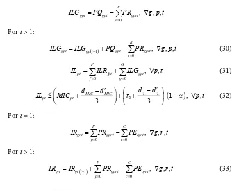
DOI: 10.4236/jcc.2018.69007 88 Journal of Computer and Communications Figure 2. Triangular fuzzy number.
Figure 3. Triangular membership function (TFN).
For t =1:
0 , , ,
R
gpt gpt gprt
r
ILG PQ PR g p t
=
= −
∑
∀For t >1:
( )1
0 , , ,
R
gpt gp t gpt gprt
r
ILG ILG − PQ PR g p t
=
= + −
∑
∀ (30)0 0 , ,
F G
pt fpt gpt
f g
IL ILR ILG p t
= =
=
∑
+∑
∀ (31)(
)
2 2
2 1 , ,
3 3
t t MIC MIC
pt pt
d d
d d
IL ≤MIC + − ′ +t + − ′ ⋅ −α ∀p t
(32)
For t =1:
0 0 , , ,
P C
grt gprt cgrt
p c
IR PR PE g r t
= =
=
∑
−∑
∀For t >1:
( )1
0 0 , , ,
P C
grt gr t gprt cgrt
p c
IR IR − PR PE g r t
= =
DOI: 10.4236/jcc.2018.69007 89 Journal of Computer and Communications
(
)
3 3
3 1 , , ,
3 3 t t MRC MRC grt gr d d d d
IR ≤MRC + − ′ +t + − ′ ⋅ −α ∀g r t
(34)
(
)
4 4
4 3
1 , , ,
3 3 PT PT gpt gp t t MPC MPC gp d d PQ PT d d d d
MPC t α g p t
′ − ⋅ + ′ − ′ − ≤ + + + ⋅ − ∀ (35)
(
)
5 55 1 , , , ,
3 3 t t MTC MTC gprt gpr d d d d
PQ ≤MTC + − ′ +t + − ′ ⋅ −α ∀g p r t
(36)
(
)
6 6
6 1 , , , ,
3 3 t t MTC MTC grct grc d d d d
PE ≤MTC + − ′ +t + − ′ ⋅ −α ∀g r c t
(37)
For t =1:
0 , , ,
3
R
D D
gct cgt cgrt
r
d d
DB D PE g c t
= ′ − = + − ∀
∑
For t >1:
( )1
0
, , ,
3
R
D D
gct gc t cgt cgrt
r
d d
DB DB − D PE g c t
=
′ −
= + + − ∀
∑
(38)1 D3 D , , ,
cgt gt cgt d d
PE DB − D c g t
′ −
≤ + + ∀
(39)
3.3. Strategy to Convert Fuzzy Objective into an Auxiliary Multiple
Objectives Linear Programming for PLP Model
Different approach is implemented for FMILP and possbilistic mixed integer linear programming (PMILP) to convert into a crisp linear programming. In this case, in order to convert PMILP into a crisp linear programming, the single fuzzy objective function is transform into a multi-objective crisp linear pro-gramming first and then possiblistic distribution is inserted into the fuzzy pa-rameters in the model.
This developed model is considered as fuzzy objective function with an insert of triangular membership function into the fuzzy coefficients. Triangular possi-bility distribution has three main values which are most possible value (cm), most
pessimistic value, (cp) and most optimistic value (co). Based on [9] theory, a
fuzzy objective function can be converted into three single equivalent auxiliary objective functions to minimize the cmx, maximize (cmx − cpx) and minimize (cox
− cmx). These three crisp equations are equivalent to minimize the possible value
DOI: 10.4236/jcc.2018.69007 90 Journal of Computer and Communications
( )
(
)
(
)
1 2 3 min min max min m m p o mz c x
zx z c c x
z c c x
=
→ = −
= −
(40)
1
0 0 0 0 0 0
0 0 0 0 0 0
0 0 0 0 0 0 0
0 0 0
min min T S F T P G m
fs fst gpt gpt t s f t p g
T P F T P G
m m
fpt pt gpt pt t p f t p g
T R G T S P F
m m
grt grt fpst fpst t r g t s p f
T P
t p r
z RMC BQ PC PQ
ILR IC ILG IC
IR HC TC BQ
= = = = = = = = = = = = = = = = = = = = = = ⋅ ⋅ ⋅ ⋅ ⋅ = ⋅ + ⋅ + + + + +
∑∑ ∑
∑ ∑ ∑
∑ ∑ ∑
∑ ∑ ∑
∑∑∑
∑∑ ∑ ∑
∑ ∑
0 0 0 0 0
0 0 0
R G T R C G
m m
gprt gprt cgrt cgrt g t r c g
T G C
m gct ct t g c
TC PR TC PE
DB DBC = = = = = = = = + + ⋅ ⋅ ⋅
∑∑
∑∑∑∑
∑∑∑
(
)
(
)
(
)
(
)
20 0 0 0 0 0
0 0 0 0 0 0
0 0 0 0 0 0 0
max max T S F T P G m p
fs fst gpt gpt gpt t s f t p g
T P F T P G
m p m p
fpt pt pt gpt pt pt t p f t p g
T R G T S P F m p
grt grt grt
t r g t s p f
z RMC BQ PC PC PQ
ILR IC IC ILG IC IC
IR HC HC TC
= = = = = = = = = = = = = = = = = = = = ⋅ + − + ⋅ − + − + − ⋅ ⋅ ⋅ + ⋅
∑ ∑ ∑
∑ ∑ ∑
∑ ∑ ∑
∑ ∑ ∑
∑∑∑
∑∑ ∑ ∑
(
)
(
)
(
)
(
)
0 0 0 0 0 0 0 0
0 0 0
m p
fpst fpst fpst
T P R G T R C G
m p m p
gprt gprt gprt cgrt cgrt cgrt t p r g t r c g
T G C
m p gct ct ct t g c
TC BQ
TC TC PR TC TC PE
DB DBC DBC
= = = = = = = = = = = ⋅ ⋅ ⋅ ⋅ − + − + − + −
∑ ∑∑∑
∑∑∑∑
∑∑∑
(
)
(
)
(
)
(
)
30 0 0 0 0 0
0 0 0 0 0 0
0 0 0 0 0 0 0
min min T S F T P G o m
fs fst gpt gpt gpt t s f t p g
T P F T P G
o m o m
fpt pt pt gpt pt pt t p f t p g
T R G T S P F o m
grt grt grt
t r g t s p f
z RMC BQ PC PC PQ
ILR IC IC ILG IC IC
IR HC HC TC
= = = = = = = = = = = = = = = = = = = = ⋅ + − + ⋅ − + − + − ⋅ ⋅ ⋅ + ⋅
∑∑ ∑
∑ ∑ ∑
∑ ∑ ∑
∑ ∑ ∑
∑∑∑
∑∑ ∑ ∑
(
)
(
)
(
)
(
)
0 0 0 0 0 0 0 0
0 0 0
o m
fpst fpst fpst
T P R G T R C G
o m o m
gprt gprt gprt cgrt cgrt cgrt t p r g t r c g
T G C
o m gct ct ct t g c
TC BQ
TC TC PR TC TC PE
DB DBC DBC
= = = = = = = = = = = ⋅ ⋅ ⋅ − + − + − + − ⋅
∑ ∑∑∑
∑∑∑∑
∑∑∑
(41)3.3.1. Treatment of the Imprecise Constraint for Fuzzy Possibilistic Model
DOI: 10.4236/jcc.2018.69007 91 Journal of Computer and Communications and Engineering field because of its direct perception characteristic and per-ceived computational efficiency [35]. This type of membership consists of low, medium and high values which are suited to apply as a parameter’s range. Prac-tically, a decision maker is experienced in estimating the value for the triangular membership function especially when there is lack of data for the imprecise variables. The upper bound of the triangular membership function is known as the most optimistic value which has very low likelihood of belonging to the set of available values; the medium value is represents the most possible value and the lower bound is the most pessimistic value.
The developed mathematical model is known as a fuzzy linear programming, which composes of a fuzzy objective function, fuzzy coefficient and fuzzy re-sources. The fuzziness of the parameter in the model can be transformed into an auxiliary crisp linear programming through apply special treatment. To trans-form the imprecise coefficient into a crisp value, weight average method is in-troduced and minimal acceptable possibility level, α = 0.5 is used. This method is applied into the supplier constraint as shown below:
1 o, 2 m, 3 p, , , , sft sf sf sf
BQ ≤w MBC ∝+w MBC ∝+w MBC ∝ ∀s f t (42)
The w1, w2 and w3 values represent the corresponding weight for the fuzzy number and for the α-cut level = 0.5, the weight is set as w w1= 3=1 6 and w2=4 6 for supplier constraint. In a real world situation, a decision mak-er is the right pmak-erson to set the α-cut value, based on their experience and exper-tise. They can adjust a higher α-cut value for the important value by assigning a greater weight for the specific value.
This fuzzy model developed has inequality constraints in the equation, and thus fuzzy ranking method is proposed in order to convert an imprecise coeffi-cient into a crisp value. This method is applied into the production constraint with using α = 0.5. The auxiliary crisp inequality is presented as follows:
,0.5 ,0.5, , , p p
gpt gp gp
PQ ⋅PT ≤MPC ∀g p t
,0.5 ,0.5, , , m m
gpt gp gp
PQ ⋅PT ≤MPC ∀g p t
,0.5 ,0.5, , , o o
gpt gp gp
PQ ⋅PT ≤MPC ∀g p t (43)
3.3.2. Strategy to Solve for Auxiliary Multi-Objective Linear Programming (MOLP) Problem
A multi-objective linear programming (MOLP) is obtained after the defuzzifica-tion process and many techniques can be applied to solve for these equadefuzzifica-tions. The possibilistic model developed in this model has a single fuzzy objective function, thus [9] method is proposed to solve for these MOLP and this ap-proach also been investigated in a real world environment in other works [15] [17] [29] [30].
DOI: 10.4236/jcc.2018.69007 92 Journal of Computer and Communications functions. The objective function for z1, z2, z3 is stated as below and the PIS and
NIS value obtained after resolve these 6 linear programming is significant for bring forward in solving next step another linear programming.
(
)
(
)
(
)
(
)
1 1 2 2 3 3 min maxmax , min
min , ax
,
m PIS m NIS m
PIS m o NIS m o
PIS p m NIS p m
z z z z
z z z z z z
z z z z z z
= =
= − = −
= − = −
(44)
Second is to construct the linear membership functions for each objective function based on the PIS and NIS value obtained.
( )
1 1
1 1
1 1 1 1 1 1 1 1 1 1 if if 0 if PIS NIS PIS NIS NIS PIS NIS z z z z
f z z z z
z z z z < − = ≤ ≤ − >
( )
2 2 2 22 2 2 2 2 2 2 2 2 1 if if 0 if PIS NIS NIS PIS PIS NIS NIS z z z z
f z z z z
z z z z > − = ≤ ≤ − <
( )
3 3 3 33 3 3 3 3 3 3 3 3 1 if if 0 if PIS NIS PIS NIS NIS PIS NIS z z z z
f z z z z
z z z z < − = ≤ ≤ − > (45)
Third is using minimum operator method to aggregate fuzzy sets in order to convert the MOLP into a single equivalent linear programming. This method will solve these three objective functions interactively and an auxiliary variable L
from the equation will provide information of level of decision maker (DM) sa-tisfaction toward the solution proposed from the programming. DM can adjust the triangular distribution based on their experience in order to achieve a higher level of satisfaction for the solution.
( )
maxs.t. , 1,2,3
0 1
g g L
L f z g
L
≤ =
≤ ≤
(46)
In this study, the equation is present as below: maxL
1
1 1 1 1 1
1
s.t. L NISzNIS PIS NIS PIS z
z z z z
≤ − ⋅
− −
2 2
2 2 2 2
1 NIS
PIS NIS PIS NIS z
L z
z z z z
≤ ⋅ − − − 3 3 3 3 3 3
1 NIS
NIS PIS NIS PIS z
L z
z z z z
≤ − ⋅
DOI: 10.4236/jcc.2018.69007 93 Journal of Computer and Communications 1
0 0 0 0 0 0 0 0 0
0 0 0 0 0 0
0 0 0 0 0 0 0 0
T S F T P G T P F
m m
fs fst gpt gpt fpt pt t s f t p g t p f
T P G T R G
m m
gpt pt grt grt t p g t r g
T S P F T P R G m
fpst fpst g t s p f t p r g
z RMC BQ PC PQ ILR IC
ILG IC IR HC
TC BQ TC
= = = = = = = = = = = = = = = = = = = = = = = = + + + + + ⋅ ⋅ ⋅ ⋅ ⋅ ⋅ +
∑∑ ∑
∑ ∑ ∑
∑ ∑ ∑
∑ ∑ ∑
∑∑∑
∑∑ ∑ ∑
∑ ∑∑∑
0 0 0 0 0 0 0 m
prt gprt
T R C G T G C
m m
cgrt cgrt gct ct t r c g t g c
PR
TC PE DB DBC
= = = = = = = ⋅ +
∑∑∑∑
⋅ +∑∑∑
⋅(
)
(
)
(
)
(
)
20 0 0 0 0 0
0 0 0 0 0 0
0 0 0 0 0 0 0 T S F T P G
m p
fs fst gpt gpt gpt t s f t p g
T P F T P G
m p m p
fpt pt pt gpt pt pt t p f t p g
T R G T S P F
m p m
grt grt grt fpst fp t r g t s p f
z RMC BQ PC PC PQ
ILR IC IC ILG IC IC
IR HC HC TC TC
= = = = = = = = = = = = = = = = = = = = + − + − ⋅ ⋅ ⋅ ⋅ ⋅ + − + − + −
∑ ∑ ∑
∑ ∑ ∑
∑ ∑ ∑
∑ ∑ ∑
∑∑∑
∑∑ ∑ ∑
(
)
(
)
(
)
(
)
0 0 0 0 0 0 0 0
0 0 0
p
st fpst
T P R G T R C G
m p m p
gprt gprt gprt cgrt cgrt cgrt t p r g t r c g
T G C
m p gct ct ct t g c
BQ
TC TC PR TC TC PE
DB DBC DBC
= = = = = = = = = = = + − ⋅ + − + ⋅ ⋅ ⋅ −
∑ ∑∑∑
∑∑∑∑
∑∑∑
(
)
(
)
(
)
(
)
30 0 0 0 0 0
0 0 0 0 0 0
0 0 0 0 0 0 0 T S F T P G
o m
fs fst gpt gpt gpt t s f t p g
T P F T P G
o m o m
fpt pt pt gpt pt pt t p f t p g
T R G T S P F
o m o
grt grt grt fpst fp t r g t s p f
z RMC BQ PC PC PQ
ILR IC IC ILG IC IC
IR HC HC TC TC
= = = = = = = = = = = = = = = = = = = = + − + − ⋅ ⋅ ⋅ ⋅ ⋅ + − + − + −
∑∑ ∑
∑ ∑ ∑
∑ ∑ ∑
∑ ∑ ∑
∑∑∑
∑∑ ∑ ∑
(
)
(
)
(
)
(
)
0 0 0 0 0 0 0 0
0 0 0
m
st fpst
T P R G T R C G
o m o m
gprt gprt gprt cgrt cgrt cgrt t p r g t r c g
T G C
o m gct ct ct t g c
BQ
TC TC PR TC TC PE
DB DBC DBC
= = = = = = = = = = = + − ⋅ + − + ⋅ ⋅ ⋅ −
∑ ∑∑∑
∑∑∑∑
∑∑∑
1 o, 2 m, 3 p, , , , sft sf sf sf
BQ ≤w MBC ∝+w MBC ∝+w MBC ∝ ∀s f t
0
1 , 2 , 3 ,
0
, , ,
R
o m p
cgt cgt cgt cgrt
r
w D ∝ w D ∝ w D ∝ = PE c g t
=
+ + =
∑
∀0 0 , ,
F G
pt fpt gpt
f g
IL ILR ILG p t
= =
=
∑
+∑
∀, ,
pt P
IL ≤MIC ∀p t
, , ,
grt gr
IR ≤MRC ∀g r t
,0.5 , , , , p p
gpt gp gp
PQ ⋅PT ≤MPC ∝ ∀g p t
,0.5 , , , , m m
gpt gp gp
PQ ⋅PT ≤MPC ∝ ∀g p t
,0.5 , , , , o o
gpt gp gp
PQ ⋅PT ≤MPC ∝ ∀g p t
1 o , 2 m, 3 p , , , , ,
gprt gpr gpr gpr
PQ ≤w MTC ∝+w MTC ∝+w MTC ∝ ∀g p r t
1 o , 2 m, 3 p, , , , ,
grct grc grt grt
DOI: 10.4236/jcc.2018.69007 94 Journal of Computer and Communications
1 , , ,
cgt gt cgt
PE ≤DB − +D ∀c g t (47)
4. Case Implementation
In this study, a complex multi-stage, multi-echelon and multi-period supply chain is developed. The first stage involves two suppliers that supply two types of raw materials to the plants. The second stage involves three production plants and they manufacture the finished products by combining the two types of raw materials together and transfer to next stage. The remaining raw materials and finish products can be stored in the inventory while waiting for process and transfer. The third stage involves three retailers that are in charge of distributing the finished products to customer based on their demand. Retailers also own their inventory and are able to store some finished products in order to over-come the fluctuation of demand situation. The planning horizon of this model is five periods and only one product is manufactured; each product is made from two units of Raw Material 1 and one unit of Raw Material 2. This fuzzy and pos-sibilistic linear programming is developed to integrate all functions involved into a chain and provide an aggregate planning over the time periods after consider-ing all the uncertainties that exist. The main focus of this model is to minimize the total operation cost. Other relevant data is stated below:
1) There is no initial inventory for the production plant and retailer’s inven-tory for time period 1.
2) Uncertain production cost for each unit includes labor cost, overtime cost and processing cost.
3) Raw material cost is constant for material 1 and material 2.
4) Each inventory space for storing the stock is limited and thus it has a maximum storage capacity for each warehouse.
5) No demand backlog is allowed at the end of time period. 6) Assuming there is no order taken in the first time period. 7) Assuming there is maximum transport capacity for each transfer.
8) A maximum violation allowed for the available fuzzy resources in the con-straint for fuzzy model is defined as approximately 10% on the right-hand side of the fuzzy constraint. This maximum tolerance value is decided by the decision maker in any systematic and non-systematic way [9].
[image:22.595.208.539.607.731.2]Table 2-8 detail the information as follows.
Table 2. Material cost data.
Material Material 1 ($/part) Material 2 ($/part)
Supplier Supplier 1 Supplier 2 Supplier 3 Supplier 1 Supplier 2 Supplier 3
Pe
ri
od
P 1 3 6 6 8 7 3
P 2 4 4 7 5 3 5
P 3 1 6 8 3 4 4
P 4 2 8 5 4 3 7
DOI: 10.4236/jcc.2018.69007 95 Journal of Computer and Communications Table 3. Supplier’s maximum supply capacity data.
Material Material 1 (part) Material 2 (part)
Supplier 1 (2000, 2300, 2750) (1500, 1800, 2000)
Supplier 2 (2100, 2400, 2850) (1400, 1700, 2050)
[image:23.595.207.540.192.258.2]Supplier 3 (2200, 2650, 2920) (1150, 1550, 1980)
Table 4. Production relates data: production cost, processing time and production capacity.
Production plant cost ($/unit) processing time (m) production capacity (unit/day)
Plant 1 (63, 70, 77) (5.0, 6.0, 6.6) (1000, 1200, 1500)
Plant 2 (58, 60, 68) (4.5, 5.2, 6.0) (870, 1080, 1470)
[image:23.595.209.539.293.410.2]Plant 3 (62, 65, 70) (3.8, 5.05, 5.8) (900, 1110, 1670)
Table 5. Type of warehouse holding cost and its inventory maximum capacity data.
Type of warehouse Inventory holding cost ($/unit) Inventory Max. capacity (unit)
Pla
nt
Warehouse 1 (1.90, 2.10, 2.30) 50
Warehouse 2 (2.30, 2.50, 2.70) 60
Warehouse 3 (1.90, 2.00, 2.30) 55
Ret
ai
ler Warehouse 1 (3.60, 4.00, 4.70) 50
Warehouse 2 (4.05, 4.50, 5.00 ) 60
Warehouse 3 (3.15, 3.50, 3.90) 50
Table 6. Transportation cost from 1 stage to another stage data.
Transportation Transportation cost ($/unit)
Supplier to plant (1.30, 1.50, 1.80)
Plant to retailer (1.35, 1.50, 1.78)
Retailer to customer (0.92, 1.00, 1.21)
Table 7. Customer order data.
Customer Period Customer demand (unit)
C
us
to
m
er
1
P 1 (0, 0, 0)
P 2 (286, 346, 394)
P 3 (114, 124, 170)
P 4 (205, 250, 301)
P 5 (314, 365, 404)
C
us
to
m
er
2
P 1 (0, 0, 0)
P 2 (238, 294, 356)
P 3 (188, 229, 270)
P 4 (220, 286, 322)
[image:23.595.211.539.442.510.2] [image:23.595.210.538.541.724.2]