ISSN Online: 2162-2086 ISSN Print: 2162-2078
Optimal Foreign Exchange Risk Hedging:
Closed Form Solutions Maximizing
Leontief Utility Function
Yun-Yeong Kim
Department of International Trade, Dankook University, Yongin-si, South Korea
Abstract
In this paper, we extend Kim (2013) [9] for the optimal foreign exchange (FX) risk hedging solution to the multiple FX rates and suggest its application method. First, the generalized optimal hedging method of selling/buying of multiple foreign currencies is introduced. Second, the cost of handling for-ward contracts is included. Third, as a criterion of hedging performance evaluation, there is consideration of the Leontief utility function, which represents the risk averseness of a hedger. Fourth, specific steps are intro-duced about what is needed to proceed with hedging. There is a computation of the weighting ratios of the optimal combinations of three conventional hedging vehicles, i.e., call/put currency options, forward contracts, and leav-ing the position open. The closed form solution of mathematical optimization may achieve a lower level of foreign exchange risk for a specified level of ex-pected return. Furthermore, there is also a suggestion provided about a pro-cedure that may be conducted in the business fields by means of Excel.
Keywords
Foreign Exchange, Risk, Optimal Hedging, Closed Form Solution
1. Introduction
Recently, foreign currency fluctuations are one of the key sources of risk in mul-tinational business/investment operations because of the widespread adoption of the floating exchange rate regime in many countries after the breakdown of the Bretton Woods system.1 The U.S. Department of Commerce has also warned
that “The volatile nature of the FX market poses a great risk of sudden and drastic 1The number of countries with floating and free floating arrangements are 36 and 29 by 2014,
re-spectively, according to IMF (https://www.imf.org/external/pubs/nft/2014/areaers/ar2014.pdf). How to cite this paper: Kim, Y.-Y. (2018)
Optimal Foreign Exchange Risk Hedging: Closed Form Solutions Maximizing Leon-tief Utility Function. Theoretical Econom-ics Letters, 8, 2893-2913.
https://doi.org/10.4236/tel.2018.814181
Received: January 24, 2018 Accepted: October 16, 2018 Published: October 19, 2018 Copyright © 2018 by author and Scientific Research Publishing Inc. This work is licensed under the Creative Commons Attribution International License (CC BY 4.0).
http://creativecommons.org/licenses/by/4.0/
Open Access
FX rate movements, which may cause significantly damaging financial losses from otherwise profitable export sales” (Trade Finance Guide, Ch. 12).2 Furthermore,
that Guide also suggested three FX risk management techniques that are consi-dered suitable for small and medium-sized enterprises companies: non-hedging FX risk management techniques, FX forward hedges, and FX options hedges.
However, for practical use by businesses or individuals, there has not been an analytical method with a closed form solution to choose from among the various available hedging tools to reduce the risk optimally, as correctly pointed out by Khoury and Chan (1988) [8]. For further studies on this issue, see Sercu and Uppal (1995) [11].
Khoury and Chan (1988) [8] gauge the preferences of finance officers in terms of the specific characteristics of a hedging tool, by relying on a questionnaire survey. Bodie, et al. (2002) [2] and Nancy (2004) [1] illustrate the technique of computerized optimization and simulation modeling to manage foreign ex-change risk. However, their techniques are not a closed form optimal hedging solution that requires additional computational burden. So its application is li-mited in the real business world. In this regard, Kim (2013) [9] introduced the optimal foreign exchange risk hedging solution by exploiting a standard portfo-lio theory.3 Hsiao (2017) [7] applies the framework of Kim (2013) [9] to
investi-gate the effects of foreign exchange exposures on the performance of Taiwan hospitality industry and try to propose some hedging strategies and strengthen their corporate risk management.
In this paper, we extend Kim (2013) [9] for the optimal single FX risk hedging solution and theory to the multiple FX rates and suggest its application method in the business fields. First, the generalized optimal hedging method of sell-ing/buying of multiple foreign currencies is introduced. Second, the cost of han-dling forward contracts is included. Third, as a criterion of hedging performance evaluation, we consider the Leontief utility (or profit for a firm) function, which represents the risk averseness of a hedger. Fourth, steps are introduced about what is needed to proceed with hedging. There is a computation of the weighting ratios of the optimal combinations of three conventional hedging vehicles, i.e., call/put currency options, forward contracts, and leaving the position open. As in the standard portfolio theory, the closed form solution of mathematical opti-mization may achieve a lower level of foreign exchange risk for a specified level of expected return. There is also a suggestion provided for a procedure that may be conducted in the business fields by means of Excel.4
The rest of this paper is as follows. Section 2 derives the expected return and return variance of the hedging vehicles. Section 3 analyzes the optimal hedging selection. Section 4 is on application of developed method, and Section 5 is the conclusion.
2U.S. Department of Commerce, Trade Finance Guide, Ch. 12, “Foreign Exchange Risk
Manage-ment,” http://trade.gov/publications/pdfs/tfg2008ch12.pdf.
3Kim (2013) [9] considered a single currency case and just for selling case. So its practical
applica-tions are very limited.
4American currency option and currency future are not considered in this paper because of the
spe-culative nature. Thus, the focus is solely on the hedging of the FX risk.
2. Expectation and Variance of Hedging Tools’ Returns
In this section, we construct an efficient hedging frontier composed of the ex-pected value and variance of each hedging vehicle’s return for the multiple for-eign exchanges. So, it is exactly matched with the portfolio possibilities curve in modern portfolio theory. Note an optimal combination of hedging vehicles is one that maximizes the expected return given a desired level of risk. For this ob-jective, there is a need to compute the mean and variance of each tool.
Before proceeding, we assume that a foreign investor needs to buy or sell
m-different currencies Θ ≡
(
θ θ1, , ,2θm)
′[
m×1]
at a future time T whereθ
iis represented by the unit of i-th currency. He is worrying about the foreign ex-change risk of domestic currency (e.g., US dollar) term translated value of Γ
and to hedge it optimally at time 0. The m-foreign exchange rates at time t in terms of domestic currency, is denoted as St≡
(
e e1t, , ,2t emt)
′. For instance,it
e is the dollar price of one euro or yen where the dollar is the domestic cur-rency. It is presupposed that there are three hedging tools, i.e., European cur-rency put (or call) option, forward contracts, and leaving the position open.5
Furthermore, there are the following definitions: a forward contract rate vector
(
1, , ,2)
t t t mt
F ≡ e e e ′, a striking price vector K≡
(
κ κ1, , ,2 κm)
′, and itspre-mium P≡
(
p p1, , ,2 pm)
′ at time t of a European put (or call) option with thecommon maturity T.6 Finally,
(
)
1, , ,2 m
C≡ c c c ′ is a per unit handling cost vector for the forward contract Ft if a bank is used.
Define the log of domestic currency term translated value of FX asset Γ at time t is given as st ≡ln
(
Θ′St)
which is a FX value. For instance, if(
10 Euro, 50 Yen)
Θ = and St =
(
1.5 Dollar Euro,0.1 Dollar Yen)
, then(
)
ln 20 Dollar
t
s = . We assume the (st) follows a random walk process: Assumption 2.1. We suppose
1 1, 1,2, ,
t t t
s+ = +s u t+ = n (2.1)
where
{ }
ut is independent, identically and normally distributed sequence withthe mean zero and variance
σ
2>0.Note E st t+1=st where Et is a conditional expectation. Thus Assumption
2.1 just a variant of the efficient FX market hypothesis.7
σ
2 is consistentlyestimated by
( )
2
2 1
ˆ n
t
t s
n
σ =
∑
= ∆ .Now we derive the return and its variance of different hedging tools, where the return is compared with the selling (or buying) a foreign currency (as a bench mark) by the spot rate s0.
2.1. FX Selling Case
First, we derive the expected return Rn and its variance Vn2 of the non-hedging
(leaving the position open), as follows.
5It is a non-hedging and to buy the foreign currency at time T.
6The value of the put option was derived by Garman and Kohlhagen (1983) [5]. 7See Diebold and Nason (1990) [3] for this issue.
Theorem 2.2. Suppose Assumption 2.1 holds. Then the expected return for non-hedging of FX asset Θ is Rn = 0 and its variance during time T is 2 2
n
V =T
σ
.All proofs of the theorems are in the Appendix.
Second, we derive the expected return Rf and its variance Vf2 of the forward
contract as follows.
Theorem 2.3. Suppose Assumption 2.1 holds. Then the expected return of forward isRf = fT− −s c0 and its variance is Vf2=0 where fT ≡ln
(
Θ′FT)
,and c≡ Θ′C Θ′S0.
Now we derive the expected return Rp and its variance Vp2 of currency put
option as follows.
Theorem 2.4. Suppose Assumption 2.1 holds. Then, (a) the expected return of currency put option is given as:
( )
( )
0 0 0
p
R = Φx z +
σ
T zφ
−pand
(b) its variance of currency put option is:
( )
(
)
( )
(
( )
( )
)
22 2 2 2
0 0 0 1 0 0 0 0
p T T
V = Φx z +T E z zσ ≥z − Φ z − xΦ z +σ T zφ . where k≡ln
(
Θ′K)
, p≡ Θ Θ′P S′ 0 , x k s0 ≡ − 0, and z0=x0(
σ T)
where( )
zφ
and Φ( )
z are the standard normal density and distribution functionsrespectively and Fa.0 denotes the distribution function of central
χ
( )2qdistri-bution with the degree of freedom q and:
(
)
( )
( )
( )
( )
( )
( )
( )
( )
2 3,0 0 2
0 2 0
1,0 0
2 2
3,0 0 3,0 0
0 0 0
2 2
1,0 0 1,0 0
1
0 1
1
1 2 1 0.
1 T T
F z
E z z z if z
F z
F z F z
z z if z
F z F z
−
≥ = ≥
−
−
= − Φ + − Φ − <
−
In the above Theorem 2.4, it was suggested that a form of 2
p
V represented by a
χ
( )21 distribution for the computation of conditional expectation(
2)
0 T T
E z z ≥z . Otherwise, there is a need for integration by a formula
(
)
( )
0
2 2
0
T T z T T T
E z z ≥z =
∫
∞zφ z dz , which requires an additional burden.Next, there is a derivation of the covariance among the three hedging tools. Note the covariance of returns between non-hedging (or option) and forward is obviously zero since the forward return is not random. Then the covariance of returns between put option and non-hedging is given as follows.
Theorem 2.5. Suppose Assumption 2.1 holds. Then the covariance of returns between put option and non-hedging is:8
( )
2(
2)
( )
0 0 0 1 0
pn T T
Cov = −xσ T zφ +T E z zσ ≥z − Φ z .
2.2. FX Buying Case
First, note we have the same expected return Rn=0 and its variance
8See Theorem 2.4 for the definitions.
2 2
n
V =T
σ
of the non-hedging, as given in Proposition 2.2 for buying a foreign exchange case.Second, we derive the expected return Rf and its variance Vf2 of forward
contract as follows.
Theorem 2.6. Suppose Assumption 2.1 holds. Then the expected return of forward9 is
0
f T
R = −s f −c
and its variance is Vf2=0.
Now we derive the expected return Rc and its variance Vc2 of currency call
option as follows.
Theorem 2.7. Suppose Assumption 2.1 holds. Then, (a) the expected return of currency call option is given as:
( )
0 0 1( )
0 cR =σ T zφ −x − Φ z −p
and
(b) its variance of currency call option is:
( )
(
)
( )
(
( )
( )
)
22 2 2 2
0 1 0 0 0 0 1 0 0
c T T
V =x − Φ z +T E z zσ <z Φ z − x − Φ z −σ T zφ
where
(
)
( )
( )
( )
( )
( )
( )
( )
( )
2 3,0 0 2
0 2 0
1,0 0
2 2
3,0 0 3,0 0
0 0 0
2 2
1,0 0 1,0 0
1
0 1
1
1 2 0.
1 T T
F z
E z z z if z
F z
F z F z
z z if z
F z F z
−
< = <
−
−
= − Φ − + Φ − ≥
−
The covariance of returns between call option and the non-hedging is given as follows.
Theorem 2.8. Suppose Assumption 2.1 holds. Then the covariance of returns between put option and non-hedging is:
( )
2(
2)
( )
0 0 0 0
cn T T
Cov =xσ T zφ +T E z zσ <z Φ z .
3. Efficient Hedging Frontier Construction
Based upon above derivation of expected return (R) and return variance (V2)
structure, now we can derive the efficient hedging frontier. It is exactly matched with the portfolio possibilities curve in a standard portfolio theory (e.g., Elton, et al. (2007) [4]).
For this purpose, first, there is consideration of a portfolio composed of non-hedging and put in the option (for FX selling) that are all risky. Let the weight of non-hedging be as w and 1-w for the option where w is a real number. Then, from the above derivation in Section 2, its expected return is defined as follows.10
( )
n(
1)
p(
1)
pR w wR= + −w R = −w R (3.1)
9Buying the foreign exchange means outflow of domestic currency. So, a negative of the forward
amount is taken.
10In case of call option,
p
R , 2
p
V and Covpn are replaced by Rc, Vc2 and Covcn respectively.
because Rn=0 for the non-hedging, and its variance is given as:
( )
(
)
2(
)
2 2 2 1 2 2 1
n p np
V w =w V + −w V + w −w Cov .
Therefore note R
( )
0 =Rp, R( )
1 =Rn =0, 2( )
0 2p
V =V and 2
( )
1 2n
V =V .
In this case, the return of forward has zero variance with the expected return, say, Rf. Thus, it is regarded as a riskless asset in the standard portfolio theory.
Now the hedging allocation line (a line of R and V)11 connecting the riskless
forward contract and a combination of non-hedging and put option is defined as follows.
( )
( )
ff
R w R
R R V
V w
−
= +
, (3.2)
where R denotes the return and V denotes the standard deviation of return (as a risk); R w R
( )
− f V w( )
is a constant slope for a given w where( )
2( )
V w = V w .
Then the efficient hedging allocation line12 is given by solving following problem:
( )
( )
max f
w
R w R V w
−
(3.3)
that is maximizing the slope of Equation (3.2) with the argument w. The prob-lem (3.3) may be solved without restriction, according to Elton, et al. ([4]: pp. 100-103), as follows.
(
)
(
) (
)
(
)
2
* 1
2 2
1 2
p f np p f
f np p n np p f
V R Cov R R
m w
m m R Cov V V Cov R R
− − −
= =
+ − + − − (3.4)
where
1 2
1
2 2
f
n np
p f
np p
R
m V Cov
R R
m Cov V
−
−
=
−
assuming
2
2 0
n np
np p
V Cov
Cov V ≠ .
If w*∉
[ ]
0,1 , then the maximization problem (3.3) should be solved underthe restriction w∈
[ ]
0,1 using a typical Kuhn-Tucker condition. Finally, the efficient hedging frontier is given by:( )
( )
*
* f f
R w R
R R V
V w
−
= +
of the left of
( ) ( )
* , *
R w V w
if w*∈
[ ]
0,1 (3.5)( ) ( )
,R w V w
= of the right of R w V w
( ) ( )
* , * otherwise.
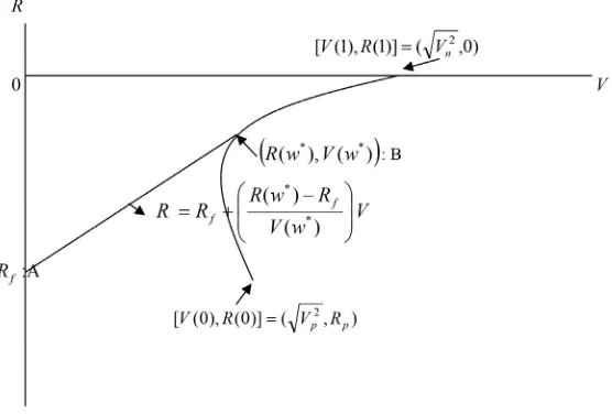
For the given efficient frontier in (3.5), the optimal hedging (cf., separation theorem) is conducted as follows. First, the hedging ratio between non-hedging and option are set as
(
w*, 1−w*)
. See Figure 1. Second, ρ is set for thefor-ward and 1−
ρ
is set for the first combination of non-hedging and option. So if1
ρ
= , then the forward becomes the unique hedging tool.Finally, ρ,w*
(
1−ρ)
, 1(
−w*)
(
1−ρ)
becomes the optimal hedging ratio of
the forward, non-hedging, and put option. Note the expected utility maximization 11It is called as the capital allocation line in the portfolio theory.
12It is called as the capital market line in the portfolio theory.
Figure 1. Efficient hedging frontier. (A: Forward only solution, B: Non-Forward solution).
may be a rule to determine an optimal ρ. The following section suggests an op-timal hedging solution through determining an opop-timal ρ under the Leontief
utility function.
4. Optimal Hedging under Leontief Utility Function
A Leontief utility (or profit for a firm) function is considered U=min ,
(
Rα β+ V)
as a criterion for hedging performance evaluation where
β
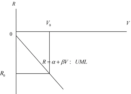
<0. Note, for the maximization of a Leontief utility function under the efficient hedging frontier in Figure 1, a pair (V, R) should satisfy a line:.
R= +
α β
V (4.1)To show it, let us derive an indifference curve. For this, suppose R0= +
α β
V0(as in Figure 2). Then a utility of
(
V R0,)
has the same utility with(
V R0, 0)
for R0≤R because a utility of
(
V R0,)
is min ,(
Rα β
+ V0)
=min ,(
R R0)
=R0while the utility of
(
V R0, 0)
is min(
R0,α β
+ V0)
=R0 from R0= +α β
V0.Simi-larly, a utility of
(
V R, 0)
has the same utility with(
V R0, 0)
for V V≤ 0 becausea utility of
(
V R, 0)
is min(
R0,α β+ V)
=R0 using α β+ V ≥ +α βV0=R0while the utility of
(
V R0, 0)
is min(
R0,α β
+ V0)
=R0 from R0 = +α β
V0. Sothe North-West direction indicates the increase of utility in a space of (V, R). Later, the above Equation (4.1) will be called a utility maximizing locus (UML). The UML might be interpreted as that which denotes how V is trans-formed into R with the same utility. It also denotes a cost of the standard devia-tion (volatility) for a hedging portfolio. See Figure 2 where the cost for the vola-tility V0 is evaluated as R0= +
α β
V0 in terms of return.Note, the above Leontief utility function and conformable UML represent an extreme risk averseness. It is related to the marginal rate of substitution of the vo-latility to a return at the utility maximizing point along UML, which is +∞, i.e., the marginal increase of V requires an infinite return increase (as compensation for augmented risk)for the same utility, whereas, a marginal decrease of V does
Figure 2. Indifference curve under Leontief utility function.
not require any return to be at the same utility level. This assumption is not so unrealistic because this model is not designed for the speculator but for the hedger/firms in the real world of business who are concerned with the volatility of fund flow.
Now to estimate α and
β
by an ordinary least square regression, were-write Equation (4.1) as:
( )
( )
2E R = +α β E z E z −
or approximately
Ti Ti Ti
R = +
α β
z − +zε
for i=1, 2, , n (4.2) where zTi≡sTi−sT i( )−1 is a change rate of FX asset during a maturity from 0 toT, z is a sample average of zTi, and
ε
Ti is assumed as a mean zero error termthat is not correlated with zTi.
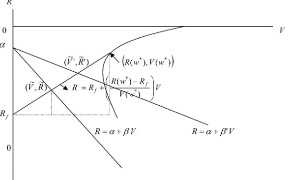
Now note the intersection of UML (4.1) and the efficient hedging frontier (3.5), which is given as follows.
( )
( )
*
* f
f
R V
R w R
V w
α
β
− =
− −
and R= +
α β
V,after solving two Equations (3.5) and (4.1) with two unknowns R and V when
*
0≤w ≤1. The above solution point
( )
V R , helps to find the optimal weight for the riskless forward contract as( )
*
*
1 V
V w
ρ = − 13 (4.3)
when 0
( )
V* 1V w
≤ ≤ . See Figure 3.
Consequently
13It is also equivalently written as
( )
* 1 R RfR w R
ρ= − − −
from the property of the proportional triangular.
Figure 3. Derivation of optimal weight for forward.
(
) (
)(
)
*,w* 1 * , 1 w* 1 *
ρ ρ ρ
− − −
(4.4)
becomes the optimal hedging ratio of forward, non-hedging, and put option us-ing (4.3) for the vector Θ. So, for instance, the weight
ρ
* of Θ needs to bedistributed to the forward.
Note, if the slope coefficient
β
as a marginal cost of volatility V is decreased toβ
′ <( )
β
, then the new optimal weight for the forward contract (riskless) isdecreased as *
( )
* *' 1 V
V w
ρ = − ′ <ρ . So more risk can be admitted because the
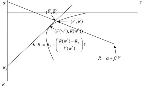
marginal cost of volatility is decreased. See Figure 3 to see this change.
However, if V is larger than V w
( )
* becauseβ
is sufficiently small, thenthe weight for the forward contract (remind Rn=0) may become zero.14 In this
case, w* is not any further an optimal weight between the leaving open position
and the option. Rather, we have to choose it from the intersection of UML and the locus of V w R w
( ) ( )
, which depends on the weight parameter w. Thenew solutions V R, for the optimization are computed as follows.15
Theorem 4.1: Suppose a pair (V, R) satisfies a line (4.1). Then
2
b b ac
R
a
− ± −
= and V =Rβ−α assuming b ac2− ≥0 where 2
2 2
2 2
p
n p pn
R
a V V Cov
β
= − − + ,
2 2 2 p
p n pn p
R
b α R V Cov R
β
= − + − ,
2 2 2 2 2
p p n
R
c α R V
β
= − .
In Theorem 4.1, we may have two different solutions that need to be selected to maximize the utility. So, we need to select one R among them maximizing the utility and define a conformable optimal expected return as
(
)
* arg max max min ,
R R
R ≡ U= Rα β+ V . See following Figure 4.
Finally, the optimal hedging ratio of the forward, non-hedging, and put op-tion becomes 0, , 1w
(
−w)
where14It is when the marginal cost of V is small and thus a riskless forward contract is not chosen. 15Remind that any forward is not used in this case.
Figure 4. Optimal hedging without forward contract.
* p
p
R R
w
R
−
= − (4.5)
from solving (3.1) for the weight w.
Finally, if
ρ
≥1, then a weighting vector (1, 0, 0)that is just selling the for-ward becomes the optimal hedging ratio.5. Application Procedures
In application, suppose, at time 0, an investor hopes to sell one unit of foreign exchange at a future time T. Then following steps need to be carried out for hedging.
1) Select three vehicles of hedging as: forward contracts, leaving the position open (Selling foreign exchange case) and European currency put option.
2) Compute mean, variance, and covariance of each tool using the formula in Section 2.
3) Compute a weighting coefficient w* as in (3.4) or w
as in (4.5) if V V< or leaving the position open against the put option.
4) Decide α and
β
using OLS regression as in (4.2).5) Compute an optimal weighting coefficient for the forward against for the portfolio of option and leaving the position open ρ as in (4.3).
6) Finally compute the optimal hedging ratio of the forward, non-hedging, and option. ρ*,w*
(
1−ρ*) (
, 1−w*)(
1−ρ*)
as in (4.4).
Consequently, we summarize the optimal weighting vectors of forward, op-tion, and non-hedging for optimal hedging, as shown in Table 1.
Then we apply the developed method for the exchange rate of the euro against the US dollar. The data frequency and period are presented on a monthly basis from January 1999 to March 2015. All data have been taken from FRED of FRB St. Louis.
Thus we assume, at time 0, i.e., June 1, 2015, 1.1235 dollar price of one euro with σ =0.024 $/€, a hedger hopes to sell one unit of foreign exchange at a
Table 1. Optimal hedging weighting vector.
* 0
w < 0≤w*<1 1≤w*
* 0
ρ < (0,0,1) 0, , 1w( −w) (0,1,0)
*
0≤ρ <1 ρ*,0, 1
(
−ρ*)
ρ*,w*
(
1−ρ*) (
, 1−w*)(
1−ρ*)
ρ*,1−ρ*,0*
1≤ρ (1,0,0) (1,0,0) (1,0,0)
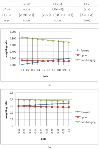
(a)
(b)
Figure 5. Optimal weighting ratio change as β decrease. (a) Selling FX case; (b) Buying FX case.
future time T = 6 months. Further we suppose that there are three hedging tools,
i.e., European currency put option, forward contracts, and leaving the position open. Assume a forward contract rate F = 1.1 $/€, selling cost for the forward
contract C = 0.1 $, a striking price K = 1.15 $/€, and its premium P = 0.03 $/€ for European put option with the maturity T = 6, respectively. Note z0= − >k s0 0
in this case.
We assume α =0.01. See Figure 5 for the optimal weighting ratio in (4.4)
change as
β
decreases16. Note, ifβ
as a marginal cost of volatility V isde-creased, then the optimal weight for the forward contract (riskless) is dede-creased, as expected in the above theoretical explication (see Section 3).
6. Conclusions
This paper introduced the optimal foreign exchange risk hedging solution by exploiting a standard portfolio theory, thus extending Kim (2013) [8] in its fol-lowing features. First, the case of the selling/buying of multiple foreign curren-cies is also considered. Second, the cost of handling forward contracts is in-cluded. Third, as a criterion of hedging performance evaluation, we consider the Leontief utility function, which represents the risk averseness of a hedger. Fourth, steps are introduced about what is needed to proceed with hedging. There is a computation of the weighting ratios of the optimal combinations of three con-ventional hedging vehicles, i.e., call/put currency options, forward contracts, and leaving the position open. The closed form solution of mathematical optimiza-tion may achieve a lower level of foreign exchange risk for a specified level of expected return. There is also a suggestion provided about a procedure that may be conducted in the business fields by means of Excel.
The structure may be extended to cover the futures and American options and it will be a future research topic for us. However, I hypothesize that a similar logic may be readily applied to these extensions applying developed method in this paper. Furthermore, a development of a convenient computer program for FX risk hedging users, based on above results, would be a useful project.
Conflicts of Interest
The author declares no conflicts of interest regarding the publication of this pa-per.
References
[1] Beneda, N. (2004) Optimal Hedging and Foreign Exchange Risk. Credit and Finan-cial Management Review, October.
[2] Bodie, Z., Kane, A. and Marcus, A. (2002) Investments. McGraw Hill, New York. [3] Diebold, F.X. and Nason, J.A. (1990) Nonparametric Exchange Rate Prediction?
Journal of International Economics, 28, 315-332.
https://doi.org/10.1016/0022-1996(90)90006-8
[4] Elton, E., Gruber, M., Brown, S. and Goetzmann, W. (2007) Modern Portfolio Theory and Investment Analysis. Wiley, New Jersey.
[5] Garman, M and Kohlhagen, S. (1983) Foreign Currency Option Values. Journal of International Money and Finance, 2, 231-237.
https://doi.org/10.1016/S0261-5606(83)80001-1
[6] Greene, W. (2003) Econometric Analysis. Pearson Education, London.
16EXCEL code for optimal hedging ratio computation is available at
https://blog.naver.com/yunyeongkim
[7] Hsiao, C.M. (2017) Enterprise Risk Management with Foreign Exchange Exposures: Evidence from Taiwan Tourism Industry. Asian Economic and Financial Review, 7, 882-906. https://doi.org/10.18488/journal.aefr.2017.79.882.906
[8] Khoury, S. and Chan, K. (1988) Hedging Foreign Exchange Risk: Selecting the Op-timal Tool. Midland Corporate Finance Journal, 5, 40-52.
[9] Kim, Y. (2013) Optimal Foreign Exchange Risk Hedging: A Mean Variance Portfo-lio Approach. Theoretical Economics Letters, 3, 1-6.
https://doi.org/10.4236/tel.2013.31001
[10] Marchand, E. (1996) Computing the Moments of a Truncated Noncentral Chi-Square Distribution. Journal of Statistical Computation and Simulation, 55, 23-29.
https://doi.org/10.1080/00949659608811746
[11] Sercu, P and Uppal, R. (1995) International Financial Markets and the Firm, South-Western.South-Western College Pub, USA.
Appendix: Proofs of Theorems
Proof of Theorem 2.2: Note the return of non-hedging is approximately the value of following17:
(
0)
0 0
T
T
S S
s s
S
′
Θ −
≅ − ′
Θ (1)
assuming Θ′
(
ST −S0)
is small. Then, under Assumption 2.1, the claimedre-sults hold as:
(
T 0)
0E s −s Ω = and
(
)
2 2 0T
E s −s Ω = Tσ . (2)
Proof of Theorem 2.3: Note the expected return for forward is the value of following:
(
0)
0 0
T
T
F S C
f s c
S
′
Θ − −
≅ − −
′
Θ (3)
assuming Θ′
(
F S CT − 0−)
is small. Its variance is obviously zero since there-turn is not random.
Proof of Theorem 2.4: (a) Note the inflow of selling weighted put option at time T is given as Θ′max
(
S KT,)
−P. Thus its return is given as following:(
)
[
] [
]
(
)
(
)
0
0
0 0
0 0 0
0 0 0
max ,
max ,
max , max ,
T
T
T T
S K P S
S
S S K S P
S S S
s s k s p x x p
′
Θ − −
′ Θ
′ ′
Θ − Θ − Θ′
= −
′ ′ ′
Θ Θ Θ
≅ − − − ≡ −
(4)
assuming ST −S0 and K S− 0 are small.
Now the expected return conditional on Ω in (4) is computed as:
(
0)
0( )
0( )
0max T,
E x x Ω − = Φ p x z +σ T zφ −p
from (4) where xT ≡sT −s0, since18
(
)
(
)
(
)
(
)
(
)
(
)
(
)
(
)
( )
( )
( )
( )
( )
( )
0 0 0 0
0 0 0
0 0 0 0
0
0 0 0
0
0 0 0
max , max , , Pr
max , , Pr
Pr , Pr
1 1
T T T T
T T T
T T T T
E x x E x x x x x x
E x x x x x x
x x x E x x x x x
z
x z T z
z
x z T z
φ σ
σ φ
Ω = < Ω <
+ ≥ Ω ≥
= < + ≥ Ω ≥
= Φ + − Φ
− Φ
= Φ +
(5)
from the definition of conditional expectation, where ~
(
0, 2)
Tx N Tσ from
Assumption 2.1 and
17It is negative for buying of foreign currency (also for the forward contract) because it means the
outflow of domestic currency.
18Note ( ) ( )
[ ]
d Pr[ ]
( )[ ]
d Pr[ ]
( | ) ( | )Pr Pr
A B
f x f x
E x x x A x x B E x A E x B
A B
=
∫
+∫
= + where x A B∈ ∪ .(
)
( )
( )
0 0 0 , 1 T T zE x x x T
z
φ σ
≥ Ω =
− Φ (6)
for the third equality (5) from Greene ([6]: p. 759), and
(
)
0(
)
( )
0 0 0
Pr Pr T Pr 1
T x x T
x x z z z
T T
σ σ
≥ = ≥ = ≥ ≡ − Φ
(7)
where zT =xT
σ
T .(b) The return’s variance of (4) is defined as:
(
)
(
)
(
)
(
)
(
)
(
(
)
)
2 0 0 2 2 0 0max , max ,
max , max ,
T T
T T
E x x E x x
E x x E x x
− Ω Ω
= Ω − Ω (8)
Note the second term of right hand side in (8) is derived from (5) directly. Then the first term of right hand side in (8) is arranged as:
(
)
(
)
(
(
)
)
(
)
(
)
(
)
(
)
(
)
(
)
(
)
( )
(
)
( )
( )
(
)
( )
2 20 0 0 0
2
0 0 0
2 2
0 0 0 0
2 2
0 0 0 0
2 2 2
0 0 0 0
max , max , , Pr
max , , Pr
Pr , Pr
, 1
1
T T T T
T T T
T T T T
T T
T T
E x x E x x x x x x
E x x x x x x
x x x E x x x x x
x z E x x x z
x z T E z zσ z z
Ω = < Ω <
+ ≥ Ω ≥
= < + ≥ Ω ≥
= Φ + ≥ Ω − Φ
= Φ + ≥ − Φ
(9) where
(
)
( )
( )
( )
( )
( )
( )
( )
( )
2 3,0 0 20 2 0
1,0 0
2 2
3,0 0 3,0 0
0 0 0
2 2
1,0 0 1,0 0
1
if 0
1
1
1 2 1 if 0
1 T T
F z
E z z z z
F z
F z F z
z z z
F z F z
−
≥ = ≥
−
−
= − Φ + − Φ − <
−
because, for the second term in last equation in (9), we may show that
(
2)
2(
2)
0 0
T T T T
E x x ≥x =T E z zσ ≥z (10)
from
(
)
(
( )
)
(
)
(
)
(
)
0 0 2 2 0 0 2 2 0 2 2 0 d d T T TT T x x T T
T T T T z z T T T g x
E x x x x x
G x x
g T z
T z T z
G z z
T E z z z
σ σ σ σ ≥ ≥ ≥ = ≥ = ≥ = ≥
∫
∫
since
(
(
)
)
0 T
T
g T z
T
G z z
σ
σ
≥ is the truncated density function of variable zT where
( )
(
)
(
(
)
)
0 0
0 0
1 d d
T T
T T
T T
x x z z
T T
g T z
g x
x T z
G x x G z z
σ σ ≥ ≥ = = ≥ ≥
∫
∫
from the change of variable formula where g and G denote the density and dis-tribution functions of xT respectively, and
σ
T zdT =dxT since zT =xTσ
Tby definition. Note zT has a standard normal, zT2 has a central
χ
( )21distribu-tion respectively. and;
Case 1: if z0≥0, then
(
2)
(
2 2 2)
(
2 2( )
02)
1,0( )
200 0 2
1,0 0 1
1 T T
T T T T
E z z z F z
E z z z E z z z
F z
− <
≥ = ≥ =
− (11)
because
(
)
(
)
(
)
[
]
(
)
[
]
(
)
2 2 2 2
0 0 0
0 0
2 2
0 2 2 0 2 2
0 0 2 0 or Pr Pr Pr Pr
T T T T T
T T
T T T T
T T
T T
E z z z E z z z z z
z z z z
E z z z E z z z
z z z z
E z z z
≥ = ≥ < −
> < −
= ≥ + < −
≥ ≥
= ≥
(12)
from
[
0]
[
0]
2 2 2 2
0 0
Pr Pr 1
2
Pr Pr
T T
T T
z z z z
z z z z
≥ < −
= =
≥ ≥
and
(
)
( )
0( )
(
)
0
2 2 2 2
0 d d 0
z
T T z T T T T T T T T
E z z ≥z =
∫
∞zφ z z =∫
−∞− z φ z z =E z z < −z (13) using the symmetry of normal distribution; and(
2 2 2)
(
2 2( )
02)
1,0( )
020 2 1,0 0 1 1 T T T T
E z z z F z
E z z z
F z
− <
≥ =
− (14)
solving following equation for
(
2 2 2)
0 T TE z z ≥z
( )
2(
2 2 2)
( )
2(
2 2 2)
( )
20 1,0 0 0 1,0 0
1=E zT =E z zT T <z F z +E z zT T ≥z 1−F z
for the final equality of (11). Further note
(
2 2 2)
3,0( )
( )
02 3,0( )
( )
3,0( )
( )
020 2 2
1,0 0 1,0 1,0 0
3 0 2 2 1 0 2 T T
F z F F z
E z z z
F z F F z
Γ −
< = =
−
Γ
(15)
from Marchand ([10]: p. 26 and Remark 4), where 1 π
2
Γ =
and
3 π
2 2
Γ =
, where
(
)
( )
( )
2
1,0 0 1,0
0,1,0 0
h =F z −F and
(
)
( )
2( )
3,0 0 3,0
0,3,0 0
h =F z −F in Marchand ([10]: p. 26 and Remark 4) where
( )
( )
1,0 0 3,0 0 0
F =F = with p = 1, α=1 and λ=0 that is a non-centrality
pa-rameter.
Plugging (15) into (11) results in
(
)
( )
( ) ( )
( )
( )
( )
2
3,0 0 2
1,0 0
2 2
1,0 0 3,0 0
2
0 2 2
1,0 0 1,0 0
1 1 1 1 T T F z F z
F z F z
E z z z
F z F z
−
−
≥ = =
− − . (16)
Case 2: z0<0
(
)
(
)
[
]
(
)
[
]
(
)
( )
(
)
( )
2 0 20 0 0 0 0
2
0 0 0
2 2 2 2
0 0 0 0
, Pr
, Pr
1 2 1
T T
T T T T
T T T T
T T T T
E z z z
E z z z z z z z z z
E z z z z z z z
E z z z z E z z z z
≥
= ≥ ≤ < − ≤ < −
+ ≥ − < − <
= < − Φ + − < − Φ −
(
)
( )
(
)
( )
(
)
( )
(
( )
)
( )
( )
( )
( )
( )
( )
( )
( )
2 2 2 2 2 2
0 0 0 0
2 2 2 2
0 1,0 0
2 2 2
0 0 2 0
1,0 0
2 2
3,0 0 3,0 0
0 0
2 2
1,0 0 1,0 0
1 2 1
1
1 2 1
1 1
1 2 1
1
T T T T
T T T T
E z z z z E z z z z
E z z z F z
E z z z z z
F z
F z F z
z z
F z F z
= < − Φ + < − Φ −
− <
= < − Φ + − Φ −
−
−
= − Φ + − Φ −
−
(17)
from (12) for the third equality, from (14) for the fourth equality and from (16) for the final equality.
Consequently we get,
(
)
(
)
(
(
)
)
( )
(
)
( )
(
( )
( )
)
2 2 2 0 0 22 2 2
0 0 0 0 0 0 0
max , max ,
1
p T T
T T
V E x x E x x
x z T E z zσ z z x z σ T zφ
= Ω − Ω
= Φ + ≥ − Φ − Φ +
from (5) and (9).
Proof of Theorem 2.5: Note the covariance between non-hedging and put option conditional on Ω is defined as:
(
)
(
)
(
)
(
)
(
)
(
)
(
)
(
)
(
)
(
)
0 0 0 0 0 0 0max , max ,
max , max ,
max , max ,
max ,
T T T
T T T
T T T T
T T
E x x p E x x p x
E x x E x x x
E x x x E x x E x
E x x x
− − − Ω Ω
= − Ω Ω
= Ω − Ω Ω
= Ω
since Emax
(
x xT, 0)
Ω is constant conditional on Ω for the secondequali-ty and the fourth equaliequali-ty holds from E x
(
T Ω =)
0.Now the claimed result is derived since
(
)
(
)
(
)
(
)
(
)
(
)
(
)
(
)
(
)
(
)
( )
(
)
( )
( )
(
)
( )
00 0 0
0 0 0
2
0 0 0 0 0
2
0 0 0 0 0
2 2
0 0 0 0
max ,
max , , Pr
max , , Pr
, Pr , Pr
, , 1
1 .
T T
T T T T
T T T T
T T T T T T
T T T T
T T
E x x x
E x x x x x x x
E x x x x x x x
x E x x x x x E x x x x x
x E x x x z E x x x z
xσ T zφ T E z zσ z z
Ω
= < Ω <
+ ≥ Ω ≥
= < Ω < + ≥ Ω ≥
= < Ω Φ + ≥ Ω − Φ
= − + ≥ − Φ
from (10) and
(
)
( )
( )
00
0 ,
T T
z
E x x x T
z
φ σ
< Ω = −
Φ (18)
from Greene ([6]: p. 759) for the last two equations.
Proof of Theorem 2.6: Note the expected return for forward is the value of following:
(
0)
0 0
T
T
S F C
s f c
S
′
Θ − −
≅ − −
′
Θ (19)
assuming F ST− 0 is small. Its variance is obviously zero since the return is not
random.
Proof of Theorem 2.7: (a) Note the outflow of buying call option at time T is given as min
(
S KT,)
+P. Thus its return normalized by S0 is given as the negative value of following:(
)
[
] [
]
(
)
(
)
0
0
0 0
0 0 0
0 0 0
min ,
min ,
min , min ,
T
T
T T
S K P S
S
S S K S P
S S S
s s k s p x x p
′
Θ + −
−
′ Θ
′ ′
Θ − Θ − Θ′
= − Θ′ Θ′ −Θ′
≅ − − − − ≡ − −
(20)
assuming ST −S0 and K S− 0 are small.
Now the expected return conditional on Ω is value of following:
(
0)
( )
0 0( )
0min T, 1
E x x p σ T zφ x z p
− Ω − = − − Φ − (21)
from (17) where xT ≡sT−s0, since
(
)
(
)
(
)
(
)
(
)
(
)
(
)
(
)
( )
( ) ( )
( )
( )
( )
0 0 0 0
0 0 0
0 0 0 0
0
0 0 0
0
0 0 0
min , min , , Pr
min , , Pr
, Pr Pr
1
1
T T T T
T T T
T T T T
E x x E x x x x x x
E x x x x x x
E x x x x x x x x
z
T z x z
z
T z x z
φ σ
σ φ
Ω = < Ω <
+ ≥ Ω ≥
= < Ω < + ≥
= − Φ + − Φ
Φ
= − + − Φ
(22)
from the definition of conditional expectation, where ~
(
0, 2)
Tx N Tσ from
Assumption 2.1 and (18) and
(
)
0(
)
( )
0 0 0
Pr Pr T Pr
T x x T
x x z z z
T T
σ σ
< = < = < ≡ Φ
(23)
where z0=x0
σ
T and zT =xTσ
T .(b) The return’s variance of call option conditional on Ω is given as:
(
)
(
)
(
)
(
)
(
)
(
(
)
)
2
0 0
2 2
0 0
min , min ,
min , min ,
T T
T T
E x x E x x
E x x E x x
− Ω Ω
= Ω − Ω (24)
Note the second term of right hand side in (24) is derived from (21) directly. Then the first term of right hand side in (24) is arranged as:
(
)
(
)
(
(
)
)
(
)
(
)
(
)
(
)
(
)
(
)
(
)
(
)
( )
( )
(
)
( )
( )
2 20 0 0 0
2
0 0 0
2 2
0 0 0 0
2 2
0 0 0 0
2 2 2
0 0 0 0
min , min , , Pr
min , , Pr
, Pr Pr
, 1
1
T T T T
T T T
T T T T
T T
T T
E x x E x x x x x x
E x x x x x x
E x x x x x x x x
E x x x z x z
T E z zσ z z x z
Ω = < Ω <
+ ≥ Ω ≥
= < Ω < + ≥
= < Ω Φ + − Φ
= < Φ + − Φ
(25) where
(
)
( )
( )
( )
( )
( )
( )
( )
( )
2 3,0 0 20 2 0
1,0 0
2 2
3,0 0 3,0 0
0 0 0
2 2
1,0 0 1,0 0
1
if 0
1
1
1 2 if 0
1 T T
F z
E z z z z
F z
F z F z
z z z
F z F z
−
< = <
−
−
= − Φ − + Φ − ≥
−
from
(
2)
2(
2)
0 0
T T T T
E x x <x =T E z zσ <z as similarly in (10) and
Case 1: z0<0
(
)
(
(
)
)
(
)
( )
( )
2 3,0 0 2
2 2 2 2
0 0 0 2
1,0 0
1 1
T T T T T T
F z
E z z z E z z z E z z z
F z
−
< = − − ≥ − = ≥ =
− (26)
From symmetry and zT has a standard normal distribution, from (12) for
the second equality, from (11) and (16) for the final equality.
Case 2: z0≥0
(
) (
)
[
]
(
)
[
]
(
)
( )
(
)
( )
( )
( )
( )
( )
( )
2 20 0 0 0 0 0
2
0 0 0
2 2 2 2
0 0 0 0
2 2
3,0 0 3,0 0
0 2 0
2 1,0 0 1,0 0 , Pr , Pr 1 2 1 1 2
1 ( )
T T T T T T
T T T T
T T T T
E z z z E z z z z z z z z z
E z z z z z z z
E z z z z E z z z z
F z F z
z z
F z F z
< = < − < < − < <
+ < < − < −
= < − Φ − + < − Φ −
−
= − Φ − + Φ −
−
(27)
from (15) and (16) for the final equality. Consequently, we get,
(
)
(
)
(
(
)
)
(
)
( )
( )
(
( )
( )
)
2 2 2 0 0 22 2 2
0 0 0 0 0 0 0
min , min ,
1 1
c T T
T T
V E x x E x x
T E z zσ z z x z σ T zφ x z
= Ω − Ω
= < Φ + − Φ − − + − Φ
from (25) and (22).
Proof of Theorem 2.8: Note the covariance between non-hedging and call option conditional on Ω is defined as:
(
)
(
)
(
)
(
)
(
)
(
)
(
)
(
)
(
)
(
)
(
)
0 0 0 0 0 0 0min , min ,
min , min ,
min , min ,
min ,
T T T
T T T
T T T T
T T
E x x p E x x p x
E x x E x x x
E x x x E x x E x
E x x x
− − − − − Ω − Ω
= − Ω Ω
= Ω − Ω Ω
= Ω
since the fourth equality holds from E x