Hyperspectral image denoising via minimizing the partial sum of singular values and superpixel segmentation

Hyperspectral Image Denoising via Minimizing the Partial

Sum of Singular Values and Superpixel Segmentation

Yang Liua, Caifeng Shanb, Quanxue Gaoa, Xinbo Gaoa, Jungong Hanc, Rongmei Cuia

a_{State Key Laboratory of Integrated Services Networks, Xidian University, Xi’an, China.}

b_{the Medical Image Analysis, Philips Research, High Tech Campus 34, Eindhoven 5656AE, NL.}

c_{the School of Computing and Communications at Lancaster University, Lancaster, UK.}

Abstract

Hyperspectral images (HSIs) are often corrupted by noise during the acquisition

pro-cess, thus degrading the HSI’s discriminative capability significantly. Therefore, HSI

denoising becomes an essential preprocess step before application. This paper

propos-es a new HSI denoising approach connecting Partial Sum of Singular Valupropos-es (PSSV)

and superpixel segmentation named as SS-PSSV, which can remove the noise

effec-tively. Based on the fact that there is a correlation between different bands of the same

signal, it is easy to know the property of low rank. To this end, PSSV is utilized, and

in order to better tap the low-rank attribute of samples, we introduce the superpixel

segmentation method, which allows samples of the same type to be grouped in the

same sub-block as much as possible. Extensive experiments display that the proposed

algorithm outperforms the state-of-the-art.

Keywords: PSSV,superpixel segmentation,hyperspectral images,

denoising

1. Introduction

In the recent years, hyperspectral images (HSIs) become more and more

popu-lar, which are being used in a wide range of fields, such as agriculture [1], terrain

classification [2], geological analysis [3], and military surveillance [4, 5]. However,

hyperspectral images often suffer from noises in the process of data acquisition, due to

5

important processing setup and significantly affects on the performance of subsequent

applications.

Recently, many HSIs’ denoising approaches have been proposed such as [6, 7, 8, 9].

As known, low-rank approximation as a powerful method is becoming more and more

10

popular in image analysis field, computer vision and web search [10, 11], or in the

denoising problem of exploring and searching low-dimensional structure from

high-dimensional data in the past years. The aim of low-rank matrix approximation-based

image recovery method is to remove the sparse noise due to the prior knowledge that

some components from the clean image are regarded as low-rank. With aid of the

15

difference between signal and noise, noise can be removed efficiently in the wavelet

domain. And meanwhile, low-rank matrix approximation methods, such as Principal

Component Analysis (PCA) [12] and matrix factorization [13, 14] are widely used to

find the best approximation of an underlying low-rank structure of data.

In the conventional PCA [12], the goodness-of-fit of data is evaluated byL2-norm,

20

which is very sensitive to outliers. To address this problem and to recover the

low-rank matrix while rejecting outliers, Robust PCA [11] improves PCA by not usingL2

-norm, so a rank minimization has been proposed and gained much interests in computer

vision [15, 16, 17]. Early works in RPCA tried to reduce the effects of outliers by

random sampling [18] or robust M-estimator [19, 20] to identify outliers or penalize

25

data with large errors. However, these methods share some limitations: either they are

sensitive to the choice of parameters, or they are not scalable enough in running time.

To further improve the above algorithms, PSSV [11] incorporated a prior information

about the target rank, which minimizes the partial sum of singular values to encourage

the target rank constraint. In view of its great advance, PSSV [11] is also exploited for

30

hyperspectral image denoising in this paper.

Motivated by the fact that PSSV [11] is successful in dynamic object, we want to

test whether it is suitable for hyperspectral images. Therefore, PSSV [11] is introduced

into our model, and we notice a fact that there is a high correlation between different

modalities from the same signal although the small difference exists, thus implying a

35

low rank property should be an appropriate prior knowledge. In order to make further

help group the same type of samples into the same sub-block as much as possible.

This paper is organized as follows: Section 2 overviews the related work and

Sec-tion 3 presents the process of hyperspectral denoising, followed by the experiments in

40

Section 4. In addition, Section 5 concludes this paper and discusses future work.

2. Related Works

In the past years, many methods have been adopted to reduce noise in HSI band

by band or pixel or pixel [21]. However, these denoising results are not satisfactory,

because the relationship between the spatial and spectral bands is not premeditated

45

simultaneously, that is to say, only the noise in spatial or spectral region is removed.

Low rank representation (LRR) has been used in HSI analysis [22]. Lu et al [23]

introduced LRR to remove stripe noise in HSI based on correlation among

differ-ent bands, and a graph regularization is considered for the local geometrical

struc-ture. Zhang [24] proposed a HSI denoising method based on low rank matrix

recov-ery(LRMR), i.e.

min

A,E ∥A∥∗+λ∥E∥1s.t.∥O−A−E∥F ≤δ (1)

whereOis the input, and aim of the model is to recover clean matrix A from O.

In [24], LRMR achieves perfect performance while the uncorrupted HSIs comply with

the low rank assumption. However, LRMR only considers that the rank is low, but does

not limit the extent of the low rank.

50

PSSV [25] extends the extent of the low rank, and the rank is accurate to a specific

number. As in [25], PSSV is proven to be effective in dynamic object. In this paper,

we will introduce PSSV into hyperspectral field, and latter experiment results show

its effectiveness. Furthermore, we also introduce the superpixel segmentation into our

model, which further improves the denoising effect.

55

3. Hyperspectral Image Denoising

3.1. superpixel segmentation

A superpixel is actually a cluster of pixels having the same type, so it can transform

Figure 1: super pixel segmentation process.

In this paper, superpixel segmentation based on entropy rate is utilized and the

60

objective function is,

max −∑

i

ui

∑

j

pi,j(A)log(pi,j(A)) +λ(−

∑

i

pzA(i)log(pzA(i))−NA) (2)

whereλis to balance the weight between the two terms,NAis the number of connected

components andu(u1, u2, ...ui, ...)satisfys a smooth distribution and wherepzA(i) =

|Si|

|V_|, i= 1,2, ..., NA. Here,Siis the i-th super pixel block,V represents a collection

of all pixels, and||indicates the number of pixels in the image block. Besides, in which

pi,j(A) =

        

ωi,j

ωi if i̸=j, and ei,j∈A

0 if i̸=j, and ei,j∈/ A

1−

∑

j:ei,j∈Aωi,j

ωi if i=j

(3)

whereei,jis an edge that connects the i-th and j-th pixels, andAis the set of edges.

Here,ωi,j = exp(− d(v1,v2)2

2σ2 ), and wherev1, v2are adjacent i-th pixel and j-th pixel,

d(v1, v2)dispalys the distance between adjacent i-th pixel and j-th pixel,σis a

param-eter set by person andωi,jis the similarity between i-th pixel and j-th pixel.

65

In this objective function, the first item ensures pixels with high similarity are

grouped into the same superpixel and the second item favors clusters with same size.

Therefore, this objective function can ensure to get both compact, homogeneous, and

balanced clusters. And the rough process is shown in Figure 1.

3.2. PSSV model

70

For each divided sub-block, it mainly contains the same type of samples, and there

adopt the PSSV [25] model to explore low rank attribute in this paper and it is the

updated version of RPCA [10]. As we know, the RPCA model was first proposed by

Ma et al. [10] and the objective is to recover clean matrixA. The formulation of this

model is the following:

min

A,Erank(A) +λ∥E∥0 s.t. O=A+E (4)

whereλis the regularization parameter. As can be seen, it is a nonconvex optimization

problem, and there is no effective solution. Generally, the problem is usually converted

into a tractable optimation problem by substituting thel0-norm for thel1-norm and the

rank for the nuclear norm, so the following optimization problem is acquired:

min

A,E∥A∥∗+λ∥E∥1 s.t.O=A+E (5)

where∥•∥_∗ is the nuclear norm(i.e., the sum of the singular values). Regarding the

solution for Eq. (5), various algorithms have been proposed, where Alternating

Direc-tion Method of Multiplier (ADMM) has shown to be quite effective. Apart from the

standard nuclear norm relaxation, there also exist some works that study variants of

nuclear norm to improve the performance of rank minimization. Among them, instead

75

of minimizing nuclear norm, PSSV [25] considers to minimize partial sum of singular

values. And it can be proven effective in dynamic object, but it is rarely used in the

field of hyperspectral, therefore, we decide to adopt it on hyperspectral images. And

the latter part of experiments also confirms its hyperspectral validity, in the following,

and PSSV will be introduced briefly.

80

At first, the idea of PSSV [25] is as:

arg min

A,E|rank(A)−N|+λ∥E∥0 s.t.O=A+E (6)

The aim of PSSV [25] is to recover a low-rank matrixAwith closing to the rank N

and a sparse matrixE. Unfortunately, the Eq. (6) is a NP-hard problem, so in order to

deal with the case, the idea of [10] is utilized to relax it with an alternative tractable

As a result, the first term of Eq. (6) is replaced with∥A∥_p=N i.e.

|rank(A)−N| ≈ |∥A∥_∗− ∥PN(A)∥_∗|

=

min(_∑n,m)

i=1

σi(A)− N

∑

i=1

σi(A)

=

min(∑n,m)

i=N+1

σi(A) =∥A∥p=N

(7)

As mentioned above, the objective function of PSSV is gained in the following:

arg min

A,E∥A∥P=N +λ∥E∥1 s.t. O=A+E (8)

In addition, the solution to this problem will be discussed in the following.

Compared with standard nuclear norm, the advantage of PSSV is that it does not

minimize the variance distribution of data with the help of target rank.

3.3. Optimization

For Eq. (8), it can be solved by ADMM proposed by Lin et al. [26]. With the help

of this method, the objective function can be evolved into the following form:

Lu(A,E,Z) =∥A∥_p=N+λ∥E∥₁+⟨Z,O−A−E⟩+₂µ∥O−A−E∥2_F (9)

whereZ∈Rm×n _{is the Lagrange multiplier, and µis a positive scalar. According}

85

to [26], Eq. (9) can be optimized by updating variable in turn while fixing the other

variables invariant, so the problem above can be divided into two subproblems.

3.3.1. SolvingA∗

From the Eq. (9), we can obtain that

A∗= arg min

A Lµk(A,Ek,Zk)

= arg min

A µk

−1_∥A∥

p=N +

1

2A−

(

O−Ek+µk−1Zk)

2

F

(10)

For Eq. (10), the Partial Singular Value Thresholding (PSVT) operator [25]PN,τ[•]

can solve the problem. As in [25], we can obtain:

Ak+1=P_N,µ−1

k (O−Ek+µ −1

where

PN,τ[Y] =UY(DY1+Sτ[DY2])VYT =Y1+UY2Sτ[DY2]VTY2, (12)

and whereDY1=diag(σ1, . . . , σN,0. . .0),DY2=diag(0, . . . ,0, σN+1, . . . , σl),

Sτ[x] =sign(x)max(|x| −τ,0)is the soft-thresholding operator [27, 28]. In

addi-90

tion, PSVT [29] enforces the target rank constraint through projection and it implicitly

encourages the resulting matrix to meet the target rank.

3.3.2. SolvingE∗

From the Eq. (9), we can obtain that

E∗= arg min

E

Lµk(Ak+1,E,Zk)

= arg min

E

λµ−_k1∥E∥₁+1

2E−(O−Ak+1+µ

−1

k Zk)

2

F

(13)

As in [28], Eq. (13) can be solved as:

Ek+1=Sλµ−_k1(O−Ak+1+µ−k1Zk) (14)

whereSτ[x] =sign(x) max(|x| −τ,0)is the soft-thresholding operator [27, 28].

Finally, the whole solution process is summarized in the following:

95

Algorithm 1Optimization

Input:O∈Rm×n, λ >0,the constraint rankN.

InitializeA0=E0=0, Zas suggested in [26],µ0>0, ρ >1andk= 0.

while do while do

1.Ak+1=PN,µ−_k1(O−Ek+µ−k1Zk).

2.Ek+1=S_λµ−1

k

(O−Ak+1+µ−_k1Zk).

end while

1.Zk+1 =Zk+µk(O−Ak+1−Ek+1).

2.µk+1=ρµk.

3.k=k+ 1.

end while

4. Experiments

To verify the effectiveness of our method, we carry out experiments on three

hy-perspectral data sets and make a comparison among the proposed algorithm with four

algorithms including LRMR [24], robust Principal Component Analysis [10], robust

Principal Component Analysis on Graphs [30], SS-LRR [31] and PSSV [25].

100

Among these contrast methods, LRMR [24] mainly adopts the low rank matrix

recovery model and regards clean samples as low-rank, robust Principal Component

Analysis [10] is an improvement for the PCA, and it adopts a rank minimization

in-stead ofL2-norm, robust Principal Component Analysis on Graphs [30] incorporates

spectral graph regularization into the Robust PCA framework, SS-LRR [31] combines

105

superpixel segmentation and low-rank representation to denoise hyperspectral image

and PSSV [25] is the update version of RPCA, minimizing partial sum of singular

values, and it is firstly used in dynamic images, rarely in hyperspectral images. As

we know, the several methods are state-of-the-art algorithms, so in order to verify the

effectiveness of proposed method, we try to compare the proposed method with them.

110

In this paper, peak signal-to-noise ratio (PSNR) and structure similarity (SSIM)

indices are used to give a quantitative assessment of the denoised results. For an HSI,

we compute the value of two indices for images on different bands, and the mean

value of these bands are calculated and denoted asM ean P SN RorM ean SSIM.

Generally speaking, higher PSNR and higher SSIM values lead to a better denoised

115

result. The definitions of two indices are as follows:

P SN Ri= 10∗log10

M N

M

∑

x=1

N

∑

y=1

[ˆui(x, y)−ui(x, y)]

2 (15)

M ean P SN R= 1

B

B

∑

i=1

P SN Ri (16)

SSIMi =

(2uuiuuˆi+C1)(2σuiuuˆi+C2) (uui

2_+u

ˆ

ui

2_+C

1)(σui

2_+σ

ˆ

ui

2_+C

2)

(17)

M ean SSIM = 1

B

B

∑

i=1

whereuianduˆirepresent theith band of the reference image and restored image,

respectively.uuianduuˆiare the average values of imageuiandˆui, whileσuiandσuˆi

are variances. AndMandNare the height and width in the spatial region, respectively.

Moreover,Bis the number of bands in spectrum region.

120

4.1. Experiment results on AVIRIS Indian Pines

In this section, the AVIRIS Indian Pines [32] are used in our experiment. The

hyper-spectral image was collected by the AVIRIS sensor over the Indian Pines region,

North-west Indiana, USA, in 1992. The scene was acquired over a mixed agricultural/forest

area, with a size of145×145×224. The bands in the wavelength range from 0.2 to

125

2.5um, nominal spectral resolution of 10nm. Furthermore, this image has a spatial

res-olution of 20mper pixel and 16-bit radiometric resolution. It includes 16 ground-truth

classes, most of which are different types of crops (e.g., corns, soybeans, and so on).

For the preconditioning of the data, the gray values of each band of the HSI are

normal-ized between [0, 1]. In the experiment, we randomly adds10%,20%,30%,40%,45% 130

salt and pepper noise to all bands. At first, in order to find the best rank, we measure

the relationship between the average peak signal-to-noise ratio and the target rank,

dis-played in Figure 2. From the figure, we can easily obtain that N=2 is the best target

rank in this data set. Similarly, we do the same operation on the ROSIS Pavia

Univer-sity Scene and Botswanna data set and besides, we obtain N=3 is the best target rank

135

in the two scenes, respectively.

1 1.5 2 2.5 3 3.5 4 4.5 5

N

54 55 56 57 58 59 60 61 62 63 64

Mean PSNR

In order to see an intuitive superpixel concept, we show the segmentation results

on Indian Pines, shown in Figure 3. From this figure, it is not hard to see that the same

type of sample is assigned to the same sub-block and samples around the border can be

effectively separated. In this way, this will help us to get a better denoising result, and

140

latter experiments also verify this view.

Figure 3: superpixel boundary map on Indian Pines.

Table 1 displays the results of mean PSNR with different methods under

differ-ent ratio of noise. It can be seen clearly that, the mean PSNR of SS-PSSV is higher

than others under10%,20%,40%,45%noise and PSSV achieves the best result

un-der30%noise, which indicates that PSSV and SS-PSSV outperform the other

meth-145

ods and are more effective in the respect of the denoising. Meanwhile, in Table 2,

the results of mean SSIM of different methods with different ratio of noise are

dis-played. From this table, we can see that SS-PSSV can obtain better performance under

20%,30%,40%,45%noise and PSSV achieves the best result under10%noise, which

suggests that SS-PSSV and PSSV are perfect and more effective in denoising. In

ad-150

dition, from Table 2, we easily get the conclusion that SS-PSSV has a more obvious

advantage over others when noise ratio is bigger, that is to say, with the increase of

noise, SS-PSSV’s denoising effect is more obvious. Under10%noise, PSSV obtains

the best performance, which indicates PSSV model is very effective in hyperspectral

field, and when superpixel is added into PSSV, SS-PSSV can get a bigger improvement,

155

process-ing. As we know, LRMR, RPCA, RPCAG and SS-LRR consider the clean sample as

a low rank ingredient, and adopt the nuclear function to portray it. Notice that nuclear

function minimizes the rank, but it does not fully utilize a prior target rank information

about samples.

160

Table 1: Mean PSNR values of the restoration results with different restoration methods on Indian Pines

Mean PSNR 10% 20% 30% 40% 45%

LRMR 41.1566 37.2959 34.6609 32.3473 31.2417

RPCA 42.4305 37.4339 31.5867 26.5500 24.4990

RPCAG 54.6674 47.7350 41.2280 34.5390 31.0893

SS-LRR 45.5827 42.2679 38.1975 36.1948 34.0037

PSSV 47.0909 45.1279 44.1626 41.2269 37.4463

SS-PSSV 55.5324 50.3469 43.2180 41.3611 37.9947

Table 2: Mean SSIM values of the restoration results with different restoration methods on Indian Pines

Mean SSIM 10% 20% 30% 40% 45%

LRMR 0.9770 0.9498 0.9172 0.8766 0.8494

RPCA 0.9946 0.9849 0.9362 0.8223 0.7537

RPCAG 0.9955 0.9934 0.9918 0.9719 0.9479

SS-LRR 0.9949 0.9933 0.9885 0.9727 0.9359

PSSV 0.9964 0.9935 0.9919 0.9834 0.9601

Figure 4: Restoration results using different methods on Indian Pines: (a) Original band 1, (b) noisy band

with ratio of40%salt and pepper noise, (c) LRMR, (d) RPCA, (e) RPCAG, (f) SS-LRR, (g) PSSV, (h)

SS-PSSV.

Figure 5: A partial enlargement of the red box in Figure 4 with (e) RPCAG, (f) SS-LRR, (g) PSSV, (h)

(a)

50 100 150 200

DN -0.1 -0.05 0 0.05 0.1 (b)

50 100 150 200

DN -0.1 -0.05 0 0.05 0.1 (c)

50 100 150 200

DN -0.1 -0.05 0 0.05 0.1 (d)

50 100 150 200

DN -0.1 -0.05 0 0.05 0.1 (e)

50 100 150 200

DN -0.1 -0.05 0 0.05 0.1 (f)

50 100 150 200

DN -0.1 -0.05 0 0.05 0.1 (g)

50 100 150 200

DN -0.1 -0.05 0 0.05 0.1

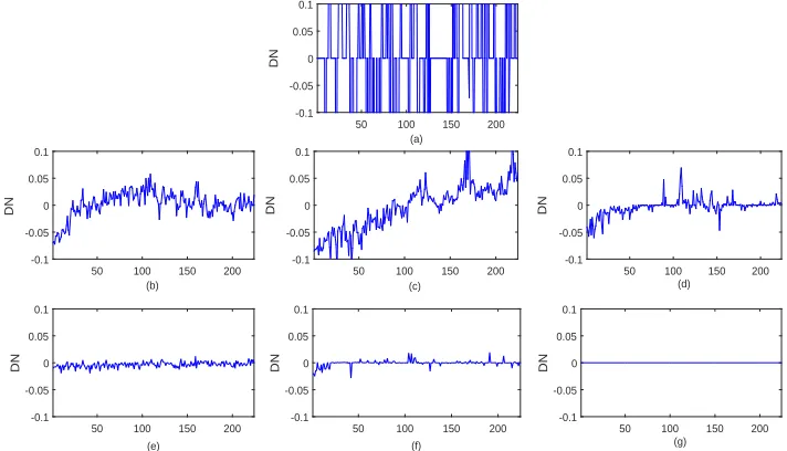
Figure 6: Difference between the noise-free spectrum and the restoration results of pixel (60,75) with ratio

of40%salt and pepper noise on Indian Pines: (a) noisy, (b) LRMR, (c) RPCA, (d) RPCAG, (e) SS-LRR, (f)

PSSV, (g) SS-PSSV.

In the following, we will show some denoised images, and Figure 4 displays the

restoration performance under40%salt and pepper noise for first band. The picture (a)

is clean image, and picture (b) is with40%salt and pepper noise. The pictures (c) to

(h) exhibit the restoration results with different methods, respectively. From the Figure

4, we can find LRMR, RPCA do not remove the noise wholly, and although RPCAG

165

remove the most noise, there is a picture overlapping problem as you see while the

restoration from SS-LRR have a fact of information loss, which can be observed easily

especially in red rectangle box. But with PSSV and SS-PSSV, the noise is basically

removed effectively while retaining most of the picture information at the same time.

In order to be able to see a clearer denoising effect, we make a partial enlargement

170

of the denoised image in Figure 5 with methods including RPCAG, SS-LRR, PSSV,

SS-PSSV. From this figure, we see clearly that (e) and (f) still exist much noise. And

is part of the residual. From (h), we can easily get that SS-PSSV achieves the best

denoising performance, which shows that the combination of superpixel segmentation

175

and PSSV makes sense.

Furthermore, the difference between the noise-free spectrum and the restoration

results in the spectral signatures at (60,75) under40%salt and pepper noise are shown

in Figure 6. From the Figure 6, we can easily see the difference is bigger in all bands

from (b),(c),(d),(e), while SS-PSSV is consistent with the original information, which

180

suggests that SS-PSSV has an advantage over others. Because SS-PSSV first adopt the

superpixel segmentation to make the same class pixel into an superpixel, and so it can

be handled as a whole.

Furthermore, in order to avoid accidental effects, we exhibit the horizonal and

ver-tical profiles of band 50 at pixel (20,30), respectively, where horizonal profiles is a

185

vector on band 50 with the second coordinate being 30 in spatial domain, and vertical

profiles is also a vector on band 50 with the first coordinate being 20 in spatial domain.

In (c) and (d) of Figure 7, we easily see that LRMR and RPCA perform poorly. And

although compared with the two model, performances of RPCAG and SS-LRR are

bet-ter, and still we can see there exist thrill in column numbers from 30 to 140 especially

190

in (f), and this phenomenon can also be found in Figure 8. In Figure 8, performances of

LRMR, RPCA, SS-LRR are bad in most row number, and compared with the models

mentioned, RPCAG performs better. However, there is a slight jitter in (e) in row

num-bers from 20 to 80. Of course, PSSV also has some glitches while SS-PSSV perform

well in almost all bands.

195

Finally, in order to get more perspective and more comprehensive comparison

a-mong several methods, PSNR values with different approaches on each band are

dis-played in Figure 9, which is under45%salt and pepper noise. From this figure, we can

see that SS-PSSV and PSSV are more high than others in most bands although there is

several rapid decline. Because we firstly adopt the superpixel segmentation, and then

200

make full use of target rank to remove noise for each superpixel. Furthermore, SSIM

values on every band are displayed in Figure 10. The larger SSIM value is, the

bet-ter denoising quality is. From the figure, we can easily see that PSSV and SS-PSSV

Column Number

20 60 100 140

DN value 0 0.2 0.4 0.6 0.8 1 Column Number

20 60 100 140

DN value 0 0.2 0.4 0.6 0.8 1 Column Number

20 60 100 140

DN value 0 0.2 0.4 0.6 0.8 1 Column Number

20 60 100 140

DN value 0 0.2 0.4 0.6 0.8 1 Column Number

20 60 100 140

DN value 0 0.2 0.4 0.6 0.8 1 Column Number

20 60 100 140

DN value 0 0.2 0.4 0.6 0.8 1 Column Number

20 60 100 140

DN value 0 0.2 0.4 0.6 0.8 1 Column Number

20 60 100 140

DN value 0 0.2 0.4 0.6 0.8 1

(a) (b) (c) (d)

(h) (g)

(f) (e)

Figure 7: Horizontal profiles of band 50 at pixel (20,30) before and after restoration on Indian Pines: (a)

Original, (b) noisy, (c) LRMR, (d) RPCA, (e) RPCAG, (f) SS-LRR, (g) PSSV, (h) SS-PSSV.

Row Number

20 60 100 140

DN value 0 0.2 0.4 0.6 0.8 1 Row Number

20 60 100 140

DN value 0 0.2 0.4 0.6 0.8 1 Row Number

20 60 100 140

DN value 0 0.2 0.4 0.6 0.8 1 Row Number

20 60 100 140

DN value 0 0.2 0.4 0.6 0.8 1 Row Number

20 60 100 140

DN value 0 0.2 0.4 0.6 0.8 1 Row Number

20 60 100 140

DN value 0 0.2 0.4 0.6 0.8 1 Row Number

20 60 100 140

DN value 0 0.2 0.4 0.6 0.8 1 Row Number

20 60 100 140

DN value 0 0.2 0.4 0.6 0.8 1

(a) (b) (c) (d)

(e) (f) (g) (h)

Figure 8: Vertical profiles of band 50 at pixel (20,30) before and after restoration on Indian Pines: (a)

Band Number

20 40 60 80 100 120 140 160 180 200 220

PSNR

0 5 10 15 20 25 30 35 40 45 50

SS-PSSV PSSV LRMR RPCA RPCAG SS-LRR

Figure 9: PSNR values of each band of the45%noise experimental results with the different restoration

methods on Indian Pines

Band Number

20 40 60 80 100 120 140 160 180 200 220

SSIM

0.65 0.7 0.75 0.8 0.85 0.9 0.95 1

SS-PSSV PSSV LRMR RPCA RPCAG SS-LRR

Figure 10: SSIM values of each band of the40%noise experimental results with the different restoration

methods on Indian Pines

In summary, AVIRIS Indian Pines contains a variety of crops and the edge between

205

crops is a curve, not a regular straight line. So if we utilize conventional rectangular

block, not using superpixel segmentation, we will not be able to deal well with

sam-ples that are around the edge. For example, PSSV segment images with conventional

advantage over PSSV in most experimental results. So in this paper, we use superpixel

210

segmentation skillfully, in this way, we can make same class of pixels into superpixel

as much as possibly. Finally, we adopt PSSV to every superpixel block which can make

full use of prior knowledge about target rank.

4.2. Experiment results on the ROSIS Pavia University Scene

In this subject, the ROSIS Pavia University scene is adopted to test the performance

215

of the proposed method. The data were collected by using the Reflective Optics System

Imaging Spectrometer sensor on the urban area of the University of Pavia, Italy [33].

This image has a size of 610*340 in pixels with a spatial resolution of 1.3mper pixel.

It altogether includes 115 spectral bands ranging from 0.43 to 0.86umin spectrum.

After discarding 12 noisy and water absorption bands, 103 bands are retained in our

220

experiment. The ground truth is classified into 9 mutually exclusive classes including

Trees, Metal sheets and so on. For the preconditioning of the data, the gray values of

each band of the HSI is normalized between [0, 1]. In experiments, we randomly adds

10%,20%,30%,40%,45%salt and pepper noise to all bands.

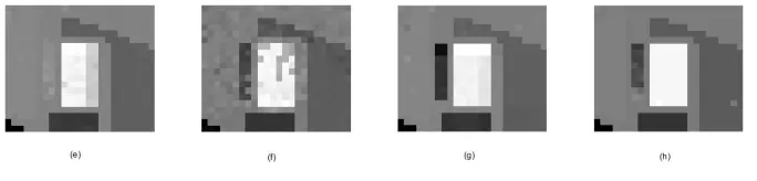
Figure 11: Restoration results using different methods on Pavia University: (a) Original band 101, (b) noisy

band with ratio of40%salt and pepper noise, (c) LRMR, (d) RPCA, (e) RPCAG, (f) SS-LRR, (g) PSSV, (h)

(a) (b) (c) (d)

(e) (f) (g) (h)

Figure 12: A partial enlargement of the red box in Figure 11.

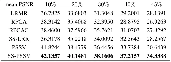
Table 3: mean PSNR values of the restoration results with different restoration methods on Pavia University

mean PSNR 10% 20% 30% 40% 45%

LRMR 36.7825 33.6803 31.3048 29.2001 28.1391

RPCA 38.3142 35.4068 32.3950 28.8795 26.9263

RPCAG 38.4600 37.5966 35.7621 31.0703 27.8292

SS-LRR 36.3178 35.2218 34.0092 32.5643 28.2567

PSSV 41.8244 38.4779 36.4456 33.7284 30.6439

SS-PSSV 42.1357 40.1481 38.1606 37.2157 34.3388

To measure the performance, mean PSNR and mean SSIM among 103 bands are

225

calculated. So Table 3 and Table 4 display the results of mean PSNR and mean SSIM

in ROSIS Pavia University Scene. From the table, it can be seen clearly that,

SS-PSSV achieves the best performance and SS-PSSV get second best result. So superpixel

Table 4: mean SSIM values of the restoration results with different restoration methods on Pavia University

mean SSIM 10% 20% 30% 40% 45%

LRMR 0.9366 0.8875 0.8323 0.7651 0.7239

RPCA 0.9725 0.9533 0.9055 0.8004 0.7183

RPCAG 0.9762 0.9617 0.9527 0.8621 0.8028

SS-LRR 0.9628 0.9537 0.9427 0.9228 0.8213

PSSV 0.9764 0.9617 0.9483 0.9111 0.8361

SS-PSSV 0.9781 0.9738 0.9668 0.9628 0.9502

In order to make a intuitive comparison, we displays restoration image on band 101

230

under40%salt and pepper noise in Figure 11. ROSIS Pavia University Scene contains

tree and so on, so if effective methods are not utilized to segment image, it will be hard

to get a good denoising result. It is obvious that traditional segmentation methods can

not effectively divide the complex image, so in this paper, we decide to adopt superpixel

segmentation, because it can handle border information well. Picture (a) is an original

235

image, and (b) shows noisy image with40% salt and pepper noise. The pictures of

(c) to (h) display restoration results with different models, respectively. From Figure

11, we can see that in the restorations with LRMR and RPCA, there has still noise

not been removed. Similarly, denoised image of RPCAG also performs poorly and

recovered image is blurred, so edge information is not preserved completely which can

240

be observed easily in red rectangle box. Simultaneously, the image of the denoising

with SS-LRR also has the phenomenon that edge information is incomplete. Only in

PSSV and SS-PSSV, the recovered image has ability to preserve edge of image and

effective removal of noise. In order to see more clearly, we have partially enlarged the

images, as shown in Figure 12.

245

In order to further explore the characteristics of hyperspectral image, we draw the

difference between the noise-free spectrum and the restoration at (300,120) under40%

salt and pepper noise. From Figure 13, we can see the difference from SS-PSSV is

Band Number

20 40 60 80 100

DN

-1 0 1

Band Number

20 40 60 80 100

DN

-1 0 1

Band Number

20 40 60 80 100

DN

-1 0 1

Band Number

20 40 60 80 100

DN

-1 0 1

Band Number

20 40 60 80 100

DN

-1 0 1

Band Number

20 40 60 80 100

DN

-1 0 1

Band Number

20 40 60 80 100

DN

-1 0 1

(a)

(b) (c) (d)

(e) (f) (g)

Figure 13: Difference between the noise-free spectrum and the restoration results of pixel (300,120) with

ratio of40%salt and pepper noise on Pavia University: (a) noisy, (b) LRMR, (c) RPCA, (d) RPCAG, (e)

SS-LRR, (f) PSSV, (g) SS-PSSV.

To further test PSSV and SS-PSSV, we calculate horizonal and vertical profiles of

250

band 96 at pixel (100,100), respectively. From Figure 14, we easily see that there is a

serious glitch on the curve in contrast models, especially more obvious in pictures (c),

(d) and (e), and this fact suggests noise is not completely removed. However, there is

no such problem in the curve of picture (g) and (h). In addition, the longitudinal curve

in Figure 15 also verifies that our argument is correct. In Figure 15, there is a more

255

serious glitch on the curve on contrast approaches and still there is no such problem in

the curve of PSSV and SS-PSSV, that is to say, the results with PSSV and SS-PSSV are

more similar to the original in most bands, which undoubtedly validates the fact that

superpixel segmentation and PSSV provide a new perspective of image processing.

For a more comprehensive result, the PSNR and SSIM values on all bands of

260

restoration with different approaches are displayed in Figure 16 and Figure 17,

always above the curves of the other methods in almost all bands and Figure 17 exists

the same solution as Figure 16, which indicates the effectiveness of superpixel

segmen-tation for removing the noise and PSSV is also beneficial to denoise in hyperspectral

265

images.

Column Number 100 200 300

DN 0 0.2 0.4 0.6 0.8 1 Column Number 100 200 300

DN 0 0.2 0.4 0.6 0.8 1 Column Number 100 200 300

DN 0 0.2 0.4 0.6 0.8 1 Column Number 100 200 300

DN 0 0.2 0.4 0.6 0.8 1 Column Number 100 200 300

DN 0 0.2 0.4 0.6 0.8 1 Column Number 100 200 300

DN 0 0.2 0.4 0.6 0.8 1 Column Number 100 200 300

DN 0 0.2 0.4 0.6 0.8 1

100 200 300

DN 0 0.2 0.4 0.6 0.8 1 (a) (d)

(e) (f) (h)

(b) (c)

(g)

Column Number

Figure 14: Horizontal profiles of band 96 at pixel (100,100) before and after restoration on Pavia University:

(a) Original, (b) noisy, (c) LRMR, (d) RPCA, (e) RPCAG, (f) SS-LRR, (g) PSSV, (h) SS-PSSV.

Row Number 200 400 600

DN 0 0.2 0.4 0.6 0.8 1 Row Number 200 400 600

DN 0 0.2 0.4 0.6 0.8 1 Row Number 200 400 600

DN 0 0.2 0.4 0.6 0.8 1 Row Number 200 400 600

DN 0 0.2 0.4 0.6 0.8 1 Row Number 200 400 600

DN 0 0.2 0.4 0.6 0.8 1 Row Number 200 400 600

DN 0 0.2 0.4 0.6 0.8 1 Row Number 200 400 600

DN 0 0.2 0.4 0.6 0.8 1 Row Number 200 400 600

DN 0 0.2 0.4 0.6 0.8 1

(a) (b) (c) (d)

(h) (g)

(f) (e)

Figure 15: Vertical profiles of band 96 at pixel (100,100) before and after restoration on Pavia University:

Table 5: mean PSNR values of the restoration results with different restoration methods on Pavia University

mean PSNR 10% 20% 30% 40% 45%

LRMR 36.2991 33.8515 31.9306 30.1682 29.2828

RPCA 37.3870 36.1057 33.7716 30.0776 27.9129

RPCAG 37.9592 37.5454 34.5579 30.9087 28.9145

SS-LRR 36.2243 35.5279 34.7330 33.6713 29.7033

PSSV 38.8750 38.1106 37.0402 34.7442 32.0922

SS-PSSV 38.2876 38.2372 35.7312 34.2281 33.7147

Table 6: mean SSIM values of the restoration results with different restoration methods on Pavia University

mean SSIM 10% 20% 30% 40% 45%

LRMR 0.9465 0.9134 0.8786 0.8357 0.8096

RPCA 0.9677 0.9606 0.9385 0.8739 0.8231

RPCAG 0.9675 0.9638 0.9539 0.9273 0.8937

SS-LRR 0.9606 0.9554 0.9486 0.9347 0.8829

PSSV 0.9676 0.9644 0.9574 0.9348 0.8940

SS-PSSV 0.9681 0.9697 0.9622 0.9434 0.9400

Band Number

10 20 30 40 50 60 70 80 90 100

PSNR

0 5 10 15 20 25 30 35 40 45 50 55

SS-PSSV PSSV LRMR RPCA RPCAG SS-LRR

Figure 16: PSNR values of each band of the10%noise experimental results with the different restoration

Band Number

10 20 30 40 50 60 70 80 90 100

SSIM

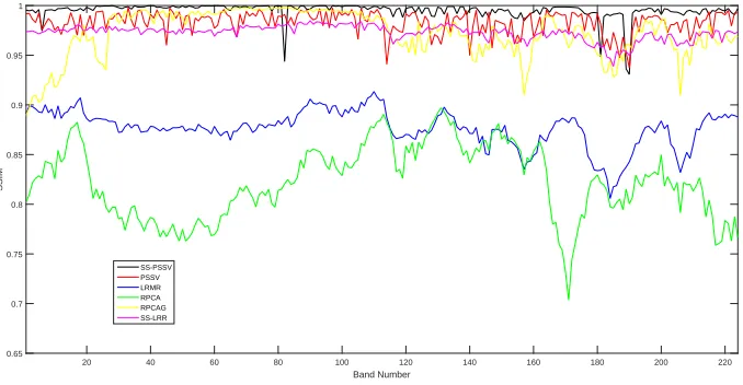
0.8 0.82 0.84 0.86 0.88 0.9 0.92 0.94 0.96 0.98 1

SS-PSSV PSSV LRMR RPCA RPCAG SS-LRR

Figure 17: SSIM values of each band of the10%noise experimental results with the different restoration

methods on Pavia University

4.3. Experiment results on the Botswanna data set

(a) (b) (c) (d) (e) (f) (g) (h)

(a) (b) (c) (d) (e) (f) (g) (h)

Figure 18: Restoration results using different methods on BOT: (a) Original band 100, (b) noisy band with

(a) (b) (c) (d) (e) (f) (g) (h)

Figure 19: A partial enlargement of the red box in Figure 18.

20 40 60 80 100 120 140

Band Number

-0.2 0 0.2

DN

20 40 60 80 100 120 140

Band Number

-0.2 0 0.2

DN

20 40 60 80 100 120 140

Band Number

-0.2 0 0.2

DN

20 40 60 80 100 120 140

Band Number

-0.2 0 0.2

DN

20 40 60 80 100 120 140

Band Number

-0.2 0 0.2

DN

20 40 60 80 100 120 140

Band Number

-0.2 0 0.2

DN

20 40 60 80 100 120 140

Band Number

-0.2 0 0.2

DN

(a)

(b) (c) (d)

(e) (f) (g)

Figure 20: Difference between the noise-free spectrum and the restoration results of pixel (60,75) with ratio

of40%salt and pepper noise on BOT: (a) noisy, (b) LRMR, (c) RPCA, (d) RPCAG, (e) SS-LRR, (f) PSSV,

Column Number

50 100 150 200 250

DN value 0 0.2 0.4 0.6 0.8 1 Column Number

50 100 150 200 250

DN value 0 0.2 0.4 0.6 0.8 1 Column Number

50 100 150 200 250

DN value 0 0.2 0.4 0.6 0.8 1 Column Number

50 100 150 200 250

DN value 0 0.2 0.4 0.6 0.8 1 Column Number

50 100 150 200 250

DN value 0 0.2 0.4 0.6 0.8 1 Column Number

50 100 150 200 250

DN value 0 0.2 0.4 0.6 0.8 1 Column Number

50 100 150 200 250

DN value 0 0.2 0.4 0.6 0.8 1 Column Number

50 100 150 200 250

DN value 0 0.2 0.4 0.6 0.8 1

(a) (b) (c) (d)

(e) (f) (g) (h)

Figure 21: Horizontal profiles of band 122 at pixel (100,80) before and after restoration on BOT: (a) Original,

(b) noisy, (c) LRMR, (d) RPCA, (e) RPCAG, (f) SS-LRR, (g) PSSV, (h) SS-PSSV.

Row Number

200 600 1000 1400

DN value 0 0.2 0.4 0.6 0.8 1 Row Number

200 600 1000 1400

DN value 0 0.2 0.4 0.6 0.8 1 Row Number

200 600 1000 1400

DN value 0 0.2 0.4 0.6 0.8 1 Row Number

200 600 1000 1400

DN value 0 0.2 0.4 0.6 0.8 1 Row Number

200 600 1000 1400

DN value 0 0.2 0.4 0.6 0.8 1 Row Number

200 600 1000 1400

DN value 0 0.2 0.4 0.6 0.8 1 Row Number

200 600 1000 1400

DN value 0 0.2 0.4 0.6 0.8 1 Row Number

200 600 1000 1400

DN value 0 0.2 0.4 0.6 0.8 1

(a) (b) (c) (d)

(e) (f) (g) (h)

Figure 22: Vertical profiles of band 122 at pixel (100,80)before and after restoration on BOT: (a) Original,

(b) noisy, (c) LRMR, (d) RPCA, (e) RPCAG, (f) SS-LRR, (g) PSSV, (h) SS-PSSV.

In our experiment, the Botswanna data set [34] is adopted, and the hyperspectral

image was acquired across Okavango Delta, Botswana(BOT). The hyperspectral data

includes two major ecosystem components defined by absence or presence of flooding,

270

namely: upland and wetland. The data set was collected in 2001 and has a size of

1476*256 with a spatial resolution of 30m in pixels, and there are altogether 1580

a hyperspectral resolution of 10nm. After discarding some noisy and water absorption

bands, 145 bands are retained for our experiment, and the ground truth is classified into

275

9 mutually exclusive classes including Water, Primary Floodplain, Riparian and so on.

Band Number

20 40 60 80 100 120 140

PSNR

0 5 10 15 20 25 30 35 40 45

SS-PSSV PSSV LRMR RPCA RPCAG SS-LRR

Figure 23: PSNR values of each band of the45%noise experimental results with the different restoration

methods on BOT.

Band Number

20 40 60 80 100 120 140

SSIM

0.4 0.5 0.6 0.7 0.8 0.9 1

SS-PSSV PSSV LRMR RPCA RPCAG SS-LRR

Figure 24: SSIM values of each band of the45%noise experimental results with the different restoration

methods on BOT.

We first calculate mean PSNR and mean SSIM, which are displayed on Table 5 and

Table 6 respectively, and two tables show the performance with several methods under

different ratio of noise. From Table 5, we can see that under20%,45% noise,

SS-PSSV achieves the best performance, and under10%,30%,40%noise, PSSV achieves

280

In Figure 18, we display recovery images on band 100 with30%salt and pepper noise

with different models. The picture (a) displays original image on band 100, and picture

(b) shows noisy graphic with ratio of30%salt and pepper noise. Pictures (c) to (h)

exhibit the restorations with different methods, respectively. From these comparisons,

285

we can see that SS-PSSV can recover a more vivid image, which can be observed easily

in red rectangle box. And an enlarged image of the red box will be shown in Figure 19.

In order to have a deeper and comprehensive understanding on spectral

signa-tures, we observe the difference between the noise-free spectrum and the restoration

at (60,75) under40%salt and pepper noise. From Figure 20, we can clearly see that

290

SS-PSSV has an big advantage over others. In order to have a more in-depth

explo-ration of botswanna data set, we records the horizontal profiles and the vertical profiles

of band 122 at pixel (100,80), and the curves are displayed in Figure 21 and Figure

22, respectively. From Figure 21, we can see that contrast methods do not handle with

noise well at column numbers between 240 and 250, while PSSV and SS-PSSV do it.

295

The same situation appear in Figure 22, because LRMR, RPCA, RPCAG, SS-LRR can

not remove noise well around row number 600, while PSSV and SS-PSSV can do.

Finally, in order to make a full understanding on all bands, PSNR and SSIM values

of restorations with different approaches on each band are displayed in Figure 23 and

Figure 24, respectively. It can be clearly seen that PSNR and SSIM values with PSSV

300

and SS-PSSV are higher than others in most bands, which indicates the effectiveness

of superpixel segmentation and PSSV for removing noise. In summary, superpixel

segmentation allows the same type of samples are divided into the same sub-block as

possible, then PSSV takes full advantage of the priori knowledge of the target rank.

When we combine the two effectively, one should get better denoising effect in theory.

305

5. Conclusions

In this work, we combine superpixel segmentation and PSSV, named as SS-PSSV.

The superpixel segmentation can obtain homogeneous regions, which can make full use

of both hyperspectral and spatial information of HSIs and PSSV makes full use of the

prior knowledge on each homogenous region, which can help remove noise effectively.

Experiments on three HSI data sets have been conducted to demonstrate that PSSV and

SS-PSSV outperforms other comparing methods in the field of hyperspectral denoising.

6. References

[1] H. Saari, A. Akuj?rvi, C. Holmlund, H. Ojanen, J. Kaivosoja, A. Nissinen,

O. Niemel?inen, Visible, very near ir and short wave ir hyperspectral drone

imag-315

ing system for agriculture and natural water applications, ISPRS - International

Archives of the Photogrammetry, Remote Sensing and Spatial Information

Sci-ences XLII-3/W3 (2017) 165–170.

[2] C. Winkens, V. Kobelt, D. Paulus, Robust features for snapshot hyperspectral

terrain-classification, in: International Conference on Computer Analysis of

Im-320

ages and Patterns, 2017, pp. 16–27.

[3] Y. Sun, Y. Zhao, K. Qin, F. Tian, P. Liu, New identification of sericite subclass

minerals using airborne hyperspectral data in the xitan region of gansu province

and its significance in gold ore prospecting, Acta Geologica Sinica 92 (1) (2018)

426–427.

325

[4] N. Ma, Y. Peng, S. Wang, P. Leong, An unsupervised deep hyperspectral anomaly

detector., Sensors 18 (3) (2018) 693.

[5] A. V. Vo, L. Truong-Hong, D. F. Laefer, D. Tiede, S. DOleire-Oltmanns, A.

Baral-di, M. Shimoni, G. Moser, D. Tuia, Processing of extremely high resolution lidar

and rgb data: Outcome of the 2015 ieee grss data fusion contestłpart b: 3-d

con-330

test, IEEE Journal of Selected Topics in Applied Earth Observations and Remote

Sensing 9 (12) (2017) 5560–5575.

[6] G. Chen, S.-E. Qian, Denoising of hyperspectral imagery using principal

com-ponent analysis and wavelet shrinkage, IEEE Transactions on Geoscience and

remote sensing 49 (3) (2011) 973–980.

[7] Q. Yuan, L. Zhang, H. Shen, Hyperspectral image denoising employing a

spectral–spatial adaptive total variation model, IEEE Transactions on Geoscience

and Remote Sensing 50 (10) (2012) 3660–3677.

[8] H. Othman, S.-E. Qian, Noise reduction of hyperspectral imagery using hybrid

spatial-spectral derivative-domain wavelet shrinkage, IEEE Transactions on

Geo-340

science and Remote Sensing 44 (2) (2006) 397–408.

[9] S.-L. Chen, X.-Y. Hu, S.-L. Peng, Hyperspectral imagery denoising using a

spatial-spectral domain mixing prior, Journal of computer science and

technol-ogy 27 (4) (2012) 851–861.

[10] E. J. Cand`es, X. Li, Y. Ma, J. Wright, Robust principal component analysis?,

345

Journal of the ACM (JACM) 58 (3) (2011) 11.

[11] E. Candes, B. Recht, Exact matrix completion via convex optimization,

Commu-nications of the ACM 55 (6) (2012) 111–119.

[12] I. Jolliffe, Principal component analysis, Wiley Online Library, 2002.

[13] R. Cabral, F. De la Torre, J. P. Costeira, A. Bernardino, Unifying nuclear

nor-350

m and bilinear factorization approaches for low-rank matrix decomposition, in:

Proceedings of the IEEE International Conference on Computer Vision, 2013,

pp. 2488–2495.

[14] Y. Shen, Z. Wen, Y. Zhang, Augmented lagrangian alternating direction method

for matrix separation based on low-rank factorization, Optimization Methods and

355

Software 29 (2) (2014) 239–263.

[15] H. Ji, C. Liu, Z. Shen, Y. Xu, Robust video denoising using low rank matrix

completion, in: Computer Vision and Pattern Recognition (CVPR), 2010 IEEE

Conference on, IEEE, 2010, pp. 1791–1798.

[16] C. A. Bishop, J. G. Liu, P. J. Mason, Hyperspectral remote sensing for mineral

360

exploration in pulang, yunnan province, china, International Journal of Remote

[17] L. Wu, A. Ganesh, B. Shi, Y. Matsushita, Y. Wang, Y. Ma, Robust photometric

stereo via low-rank matrix completion and recovery, Computer Vision–ACCV

2010 (2011) 703–717.

365

[18] B. Fischler, Martin A, R. C, Random sample consensus: a paradigm for model

fitting with applications to image analysis and automated cartography,

Commu-nications of the ACM 24 (6) (1981) 381–395.

[19] Y.-Q. Zhao, P. Gong, Q. Pan, Object detection by spectropolarimeteric imagery

fusion, IEEE Transactions on Geoscience and Remote Sensing 46 (10) (2008)

370

3337–3345.

[20] F. De La Torre, M. J. Black, A framework for robust subspace learning,

Interna-tional Journal of Computer Vision 54 (1) (2003) 117–142.

[21] Y. Q. Zhao, J. Yang, Hyperspectral image denoising via sparse representation

and low-rank constraint, IEEE Transactions on Geoscience and Remote Sensing

375

53 (1) (2015) 296–308.

[22] H. Huang, A. G. Christodoulou, W. Sun, Super-resolution hyperspectral imaging

with unknown blurring by low-rank and group-sparse modeling, in: IEEE

Inter-national Conference on Image Processing, 2014, pp. 2155–2159.

[23] X. Lu, Y. Wang, Y. Yuan, Graph-regularized low-rank representation for

destrip-380

ing of hyperspectral images, IEEE Transactions on Geoscience and Remote

Sens-ing 51 (7) (2013) 4009–4018.

[24] H. Zhang, W. He, L. Zhang, H. Shen, Q. Yuan, Hyperspectral image restoration

using low-rank matrix recovery, IEEE Transactions on Geoscience and Remote

Sensing 52 (8) (2014) 4729–4743.

385

[25] T.-H. Oh, Y.-W. Tai, J.-C. Bazin, H. Kim, I. S. Kweon, Partial sum minimization

of singular values in robust pca: Algorithm and applications, IEEE transactions

[26] Z. Lin, M. Chen, Y. Ma, The augmented lagrange multiplier method for exact

recovery of corrupted low-rank matrices, arXiv preprint arXiv:1009.5055.

390

[27] D. L. Donoho, I. M. Johnstone, Adapting to unknown smoothness via wavelet

shrinkage, Journal of the american statistical association 90 (432) (1995) 1200–

1224.

[28] E. T. Hale, W. Yin, Y. Zhang, Fixed-point continuation for L1-minimization:

Methodology and convergence, SIAM Journal on Optimization 19 (3) (2008)

395

1107–1130.

[29] E. M. de S´a, Exposed faces and duality for symmetric and unitarily invariant

norms, Linear Algebra and its Applications 197 (1994) 429–450.

[30] N. Shahid, V. Kalofolias, X. Bresson, M. Bronstein, P. Vandergheynst, Robust

principal component analysis on graphs, in: Proceedings of the IEEE

Internation-400

al Conference on Computer Vision, 2015, pp. 2812–2820.

[31] J. Ma, C. Li, Y. Ma, Z. Wang, Hyperspectral image denoising based on low-rank

representation and superpixel segmentation, in: Image Processing (ICIP), 2016

IEEE International Conference on, IEEE, 2016, pp. 3086–3090.

[32] D. Landgrebe, Aviris nw indianas indian pines 1992 data set, 1992.

405

[33] A. Plaza, J. A. Benediktsson, J. W. Boardman, J. Brazile, L. Bruzzone, G.

Camps-Valls, J. Chanussot, M. Fauvel, P. Gamba, A. Gualtieri, et al., Recent advances in

techniques for hyperspectral image processing, Remote sensing of environment

113 (2009) S110–S122.

[34] A. L. Neuenschwander, Remote sensing of vegetation dynamics in response to

410

flooding and fire in the Okavango Delta, Botswana, The University of Texas at