Attention module-based spatial temporal graph convolutional
1
networks for skeleton-based action recognition
2 3
Yinghui Kong,a Li Li,a Ke Zhang,a Qiang Ni,b Jungong Hanb 4
a
North China Electric Power University, Department of Electronic and Communication Engineering, North 5
Yonghua Road #619, Baoding, China, 071000 6
b
Lancaster University, School of Computing and Communications, Bailrigg, Lancaster, United Kingdom, LA1 4YW 7
8
Abstract. Skeleton-based action recognition is a significant direction of human action recognition, because the 9
skeleton contains important information for recognizing action. The spatial temporal graph convolutional networks 10
(ST-GCN) automatically learn both the temporal and spatial features from the skeleton data, and achieve remarkable 11
performance for skeleton-based action recognition. However, ST-GCN just learn local information on a certain 12
neighborhood, but does not capture the correlation information between all joints (i.e., global information). 13
Therefore, we need to introduce global information into the spatial temporal graph convolutional networks. In this 14
work, we propose a model of dynamic skeletons called attention module-based Spatial Temporal Graph 15
Convolutional Networks (AM-STGCN), which solves these problems by adding attention module. The attention 16
module can capture some global information, which brings stronger expressive power and generalization capability. 17
Experimental results on two large-scale datasets, Kinetics and NTU-RGB+D, demonstrate that our model achieves 18
significant improvements over previous representative methods. 19
20
Keywords: action recognition, spatial temporal graph convolution network, non-local neural network, attention 21
module. 22
23
*Yinghui Kong, E-mail: [email protected] 24
25 26
1 Introduction 27
Action recognition technology plays an increasingly important role in many fields such as 28
intelligent monitoring, human-computer interaction, video sequence understanding, and medical 29
health. Video action recognition technology is challenged by factors such as occlusion, dynamic 30
background, mobile camera, angle of view and illumination change. 31
Before the advent of deep learning, the best algorithm for human action recognition in video 32
was iDT1,2, and the subsequent works were basically improved based on the iDT method. Human 33
action recognition uses multiple modalities of data such as appearance, depth, optical flows, and 34
performance in image understanding tasks, more and more researchers are beginning to use deep 36
learning methods to solve the problem of video analysis. Action recognition methods based on 37
RGB video or optical flows, such as Two-Stream4,5, C3D6, I3D7, RNN8methods, are greatly 38
affected by illumination, scene and camera lens movement, so it is difficult to describe the 39
motion of the human body in the sequence, the recognition performance in some complex 40
datasets needs to be improved. In recent years, due to the cost reduction of depth sensors (such as 41
Kinect) and the emergence of real-time human pose estimation algorithms, skeleton-based action 42
recognition has become more and more popular. 43
Skeleton-based action recognition methods have been widely studied and paid attention due 44
to its strong adaptability to dynamic environments and complex backgrounds. Traditional 45
methods9,10 require hand-crafted features and traversal rules, which are less efficient. Ordinary 46
deep learning-based methods11-20 manually structure the skeleton into joint coordinate vectors or 47
pseudo-images, which are then sent to the RNN or CNN network for prediction of the action 48
categories. The human skeleton is naturally constructed as a graph in a non-Euclidean space, in 49
which the joint acts as a node, and the edge is constructed according to the natural connection 50
relationship of the human body. Recently, the Graph Convolutional Networks (GCN) have 51
extended convolution operations from images to graph structures, and have been successfully 52
applied to many applications. For skeleton-based action recognition, GCN-based methods 53
contain ST-GCN3, STGC21, SR-TSL22, AGCN23, PB-GCN24, GR-GCN25 and DPRL+GCNN26. 54
ST-GCN applied GCN for skeleton-based action recognition task and directly model the original 55
skeleton data, it extended graph neural networks to a spatial-temporal graph model, and obtained 56
better action representations. Compared to ordinary deep learning-based methods, GCN-based 57
in the ST-GCN method is performed on the 1-neighbor of the root node and cannot capture 59
global information. For the action categories in which the interaction joints are not in the same 60
neighborhood, such as brushing, clapping, but there are relations between these nonadjacent 61
joints, attention mechanism can learn these relations. Paying more attention to those joints may 62
improve recognition performance. Attention modules that work well include non-local neural
63
networks27, Interaction-aware attention28, CBAM29, SENet30 etc.
64
In order to solve this problem, we propose an improved method based on ST-GCN, which is 65
attention module-based Spatial Temporal Graph Convolutional Networks (AM-STGCN). 66
Attention module helps the model focus on all positions and learn different weights for each 67
position. In AM-STGCN, we add the non-local neural network as an attention module after the 68
convolution operation of the baseline model ST-GCN to learn the feature representation with 69
long-range dependencies. In addition, we discussed the effects of adding attention blocks to 70
different layers, as well as the effects of adding multiple attention blocks. We did a lot of 71
experimentation and analysis, and finally got the best strategy. The experimental results on two 72
large-scale action recognition datasets Kinetics31 and NTU-RGB+D32 show that AM-STGCN can 73
significantly outperform ST-GCN in action recognition. 74
In the remainder of the paper, we first provide some related work in Sec. 2, and then 75
introduce the original ST-GCN model and our AM-STGCN model in Sec. 3. We summarize and 76
analyze the experimental results in Sec. 4. Finally, we draw conclusions and point out future 77
2 Related Work 79
2.1 Action Recognition Based on RGB Video or Optical Flows
80
Most previous studies were based on RGB video or optical flows. Traditional action recognition 81
methods are mostly based on optical flows, and the representative algorithm is iDT1,2. DT 82
algorithm utilize optical flow field to obtain some trajectories in the video sequence, then extract 83
the HOF, HOG, MBH and trajectory characteristics along the trajectory. IDT improves dense 84
trajectories by explicitly estimating camera motion. Then, some methods based on deep learning 85
gradually appeared, and their performance was much better than traditional methods. Two-86
stream method was originally proposed by Simonyan et al.4, and Feichtenhofer et al.5 improved 87
the model. Two-stream method utilizes both appearance and optical flows information: in spatial 88
stream, in the form of appearance on a single frame, the scene and target information depicted by 89
video are carried; in temporal stream, the motion of the observer (camera) and the target are 90
expressed in the form of multi-frame optical flows. Tran et al.6 adopted 3D convolution and 3D 91
pooling to construct a network, which can directly process video, and its efficiency is much 92
higher than other methods. Carreira et al.7 proposed a model named “I3D” based on Inceptionv1, 93
which inflates Inceptionv1’s filters and pooling kernels into 3D, leading to very deep, naturally 94
spatiotemporal classifiers. Du et al.8
introduced a novel pose-attention mechanism to adaptively 95
learn pose-related features at every time-step action prediction of RNNs. 96
Although action recognition methods based on RGB video or optical flows perform high 97
performance, there are still some problems. For example, it is susceptible to background, 98
illumination and appearance changes, and extract optical flow information requires high 99
2.2 Skeleton-based Action Recognition
101
The human skeleton can provide a very good representation of the human body motions, which 102
is beneficial to the analysis of human actions. On the one hand, skeleton data is inherently robust 103
in background noise, and provides abstract and high-level features of human motion. On the 104
other hand, the size of the skeleton data is very small compared to RGB data, which allows us to 105
design a lightweight and hardware-friendly model. 106
Skeleton-based action recognition approaches can be categorized into traditional methods 107
and deep learning methods. Deep learning methods contain RNN based methods, CNN based 108
methods and graph convolutional network (GCN) based methods. 109
Some traditional methods shown in Refs. 9 and 10 require hand-crafted features and traversal 110
rules to achieve skeleton action recognition. With the development of deep learning, RNN based 111
methods appears gradually. Du et al.11 divided the human skeleton into five parts according to 112
human physical structure, and then separately feeded them to five bidirectionally recurrently 113
connected subnets. Song et al.12 proposed an end-to-end spatial and temporal attention model, 114
which learns to selectively focus on discriminative joints of skeleton within each frame of the 115
inputs and pays different levels of attention to the outputs of different frames. Zhang et al.13 116
designed a view adaptive recurrent neural network (RNN) with LSTM architecture, which 117
enables the network itself to adapt to the most suitable observation viewpoints from end to end. 118
In recent years, a number of CNN based approaches have also emerged. Kim et al.14 re-designed 119
the original TCN by factoring out the deeper layers into additive residual terms which yields 120
both interpretable hidden representations and model parameters. Liu et al.15 proposed an 121
enhanced skeleton visualization method to represent a skeleton sequence as a series of visual and 122
compact yet distinctive manner. Li et al.16 designed a novel skeleton transformer module to 124
rearrange and select important skeleton joints automatically. Li et al.17 proposed an end-to-end 125
convolutional co-occurrence feature learning framework to aggregate different levels of 126
contextual information. Liu et al.18 proposed a recurrent attention mechanism for their
GCA-127
LSTM network, which is able to selectively focus on the informative joints in the action
128
sequence with the assistance of global contextual information. Xie et al.19 designed a
temporal-129
then-spatial recalibration scheme, resulting in an end-to-end Memory Attention Networks
130
(MANs) which consist of a Temporal Attention Recalibration Module (TARM) and a
Spatio-131
Temporal Convolution Module (STCM). Zheng et al.20 designed an adaptive attentional module
132
to focus attention on the most discriminative parts in the single skeleton. Although RNN based 133
methods has a strong ability to model sequence data, and CNN based methods has good 134
parallelism and easier training process, however, neither CNN nor RNN fully represent the 135
structure of the skeleton. 136
Recently, some methods based on graph convolution have appeared, and the effect has been 137
improved obviously. Yan et al.3 directly simulated the original skeleton using the graph 138
convolution, which eliminates the need for manual part assignment, and it is easier to design and 139
potent to learn better action representations. Li et al.21 designed multi-scale convolutional filters 140
to encode the graph structure data, and proposed a recursive graph convolution model. Si et al.22 141
utilized a spatial reasoning network to capture the high-level spatial structural features within 142
each frame, and utilized a composition of multiple skip-clip LSTMs to model the detailed 143
temporal dynamics of skeleton sequences. In order to design individual graphs for different 144
samples, Shi et al.23 introduced non-local neural networks into graph convolution operation to 145
Thakkar et al.24 divided the skeleton graph into four subgraphs, and used relative coordinates and 147
temporal displacements as features at each node instead of 3D joint coordinates which improves 148
action recognition performance. Gao et al.25 constructed a generalized graph via spectral graph 149
theory to capture the space-time variation. Tang et al.26 proposed a deep progressive
150
reinforcement learning (DPRL) method to extract key frames, and employed the graph-based
151
convolutional neural network to capture the dependency between the joints for action recognition.
152
3 Methodology 153
We briefly describe the original spatial temporal graph convolutional networks (ST-GCN) in Sec. 154
3.1. And in Sec. 3.2, we give a briefly description about the methods of utilizing the attention 155
module to boost the performance, and propose the improved model -- attention module-based 156
spatial temporal graph convolution network (AM-STGCN). 157
3.1 Spatial-Temporal Graph Convolutional Networks (ST-GCN)
158
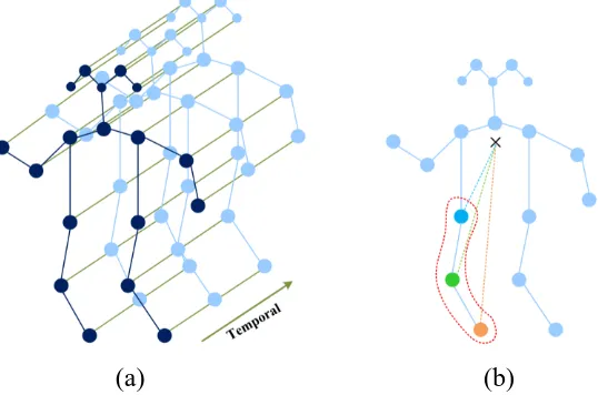
As shown in Ref. 3, the authors take joints as nodes and the connections between nodes as edges 159
to construct the skeleton graph. Fig. 1 (a) shows an example of a spatial-temporal skeleton graph. 160
In one frame, the natural connections between the joints (i.e., the human bones) act as spatial 161
edges; in adjacent frames, the same joints are joined as temporal edges. The property of each 162
node is the coordinate vector of the joint. Multi-layers spatial-temporal graph convolution 163
operation is applied to the spatial-temporal skeleton graph to obtain advanced feature map, and 164
then use the SoftMax classifier to predict the action category. 165
ST-GCN applies the spatial configuration partitioning strategy shown in Fig. 1(b) in frame. 166
The spatial configuration partitioning strategy divides the node's 1-neighbor into three subsets: 1) 167
the gravity center of the skeleton (black cross); 3) the centrifugation subset (yellow dots): the 169
neighboring nodes that are further to the gravity center of the skeleton. Each color in the Fig. 1(b) 170
corresponds to a specific learnable weight vector. The authors of ST-GCN propose three 171
partitioning strategy, and it has been proved that the spatial configuration partitioning strategy 172
shown in Fig. 1(b) is the best, so this work directly adopts this strategy. 173
[image:8.612.173.442.214.392.2]174 175
Fig. 1 (a) Spatial temporal graph of the skeleton. (b) Partitioning strategy, different colors represent different 176
subsets. 177
Spatial graph convolution is formulated as: 178 )) ( ( ) ( ) ( 1 ) ( ) ( tj ti tj in v B
v ti tj ti
out f v w l v
v Z v f ti tj
, (1)
179
where f is the feature map. vtiis the node of the graph. B(vti) is the sampling area, which is 180
defined as the 1-neighbor set of joint nodes. The neighbor set B(vti)of a joint node vtiis 181
partitioned into a fixed number of K subsets, where each subset has a numeric label.3 The 182
mapping function ltimaps a node in the neighborhood to its subset label. The weight function w
183
gives different weights according to different ltivalues. The normalizing term Zi(vj) equals the
184
cardinality of the corresponding subset. 185
To model the spatial temporal dynamics within skeleton sequence, since the number of 186
neighbors per node is fixed at 2 (the corresponding joint in the previous and subsequent frames), 187
it is directly to perform the graph convolution similar to the classical convolution operation, 188
concretely, we perform a Kt1 convolution on the output feature map computed above.23 189
In the single frame case, ST-GCN with the spatial configuration partitioning strategy can be 190
implemented with the following formula: 191
j j in j j j jout f W
f ( 2)
1 2 1
. (2)
192
In formula 2, f is the CinTV feature map where V denotes the number of nodes, T denotes the 193
temporal length and Cindenotes the number of input channels. A is the 18183 adjacency 194
matrix, whose element Aij indicates whether the node vi is in the subset of node vj. 0 195
denotes the self-connections of vertexes, 1 denotes the connections of centripetal subset 196
and2denotes the centrifugal subset.
kki j ii
j (A ) is the normalized diagonal matrix, α is 197
set to 0.001 to avoid the empty rows in A. Wj is the CoutCin11 weight vector of 198
the 11 convolution operation. M is a VV learnable attention map which indicates the 199
importance of each node. denotes the element-wise product between two matrixes. This
200
means that if one of the elements in A is 0, then whatever the value of M is, it will always be 0.
201
So M just operates in the 1-neighbor of the root node.
202
3.2 Attention Module-based Spatial Temporal Graph Convolution Network
203
In the spatial temporal graph convolution model, the receptive field of the convolution operation 204
is the 1-neighbor of the root node, so it only captures local features. However, in different 205
neighbor of the joint. For example, for many actions such as combing hair, brushing teeth, the 207
relationship between the hand and the head may be important. In order to solve this problem, we 208
introduce the idea of non-local neural network27, make some improvements to the ST-GCN 209
model, and then propose AM-STGCN skeleton-based action recognition method based on the 210
non-local attention mechanism, which directly focuses on the features of all joints, and get more 211
efficient features by attention operations. 212
213 214
[image:10.612.86.503.242.610.2]215
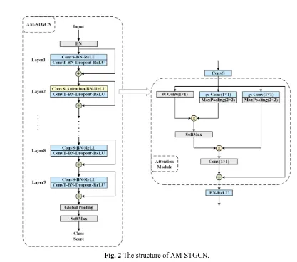
Fig. 2 The structure of AM-STGCN. 216
Fig. 2 shows the network structure of AM-STGCN, where we add the attention module after 217
the spatial convolution operation (ConvS) of Layer2. The model consists of nine layers of spatial 218
temporal graph convolution operators. The first three layers have 64 output channels, the middle 219
layer of AM-STGCN includes the spatial convolution operation (ConvS) and the temporal 221
convolution operation (ConvT). The residual connection33 is added on each layer. 222
Non-local neural network is a versatile, flexible building block, it can be easily embedded 223
into existing 2D and 3D convolutional networks to improve or visualize related CV tasks. This 224
allows us to combine global and local information to build richer hierarchy. In Fig. 2, the right 225
side is our attention module, which is used to capture the correlation between all joints. We 226
construct the attention module mainly following the idea of non-local neural network: first, linear 227
mapping is conducted on the feature map of ConvS , which is implemented as 1×1 convolution, 228
and then get the θ, φ, g features; second, we perform a matrix point multiplication operation on 229
θ and φ to calculate the autocorrelation in the feature, and then carry out Softmax operation to 230
obtain the self-attention coefficient; third, the attention coefficient is multiplied back into the 231
feature matrix g;at last, residual connection is established with the original input feature map, 232
and then we get a new set of features. Specifically, we add 2×2 MaxPooling operation after θ, 233
φ features to reduce computational cost. Such an attention module is called one attention block, 234
and multiple attention blocks will be used in the work. How many attention blocks are added to 235
the model and where they are added will be analyzed in detail in Sec. 4, and the experimental 236
results are given at the same time. 237
4 Experiments and Analysis 238
In this section, we evaluate the performance of the AM-STGCN model. In order to compare with 239
the baseline model ST-GCN, our experiments are performed on the same two large-scale action 240
recognition datasets: the human action dataset Kinetics31 is the largest unconstrained action 241
action recognition dataset. First, we conduct a detailed ablation study of the Kinetics dataset to 243
analyze the contribution of the proposed model to recognition performance. Then, the 244
corresponding experiments are carried out on the NTU-RGB+D dataset to verify whether the 245
proposed model has certain generalization ability. Finally, we compare AM-STGCN with ST-246
GCN and some state-of-the-art results of skeleton-based action recognition on Kinetics and 247
NTU-RGB+D. All experiments were performed on PyTorch deep learning framework using two 248
1080Ti GPUs. 249
4.1 Datasets
250
Kinetics31: Kinetics is a large human action dataset that contains 400 action classes taken from 251
different YouTube video, each class with at least 400 video clips, each clip lasts about 10 252
seconds31. These actions include the interaction between people and objects, such as playing an 253
instrument, and the interaction between people, such as shaking hands. 254
The Kinetics dataset only provides raw video clips and does not provide skeleton joint data. 255
As shown in Ref. 3, they use the public available OpenPose34 toolbox to estimate the location of 256
18 joints on every frame of the clips. In this work, we use the Kinetics-skeleton dataset provided 257
by the author of ST-GCN, which marks the position of 18 joints in each frame. The dataset 258
provides a training set of 240,000 clips and a validation set of 20,000 clips. In accordance with 259
the recommendations in Ref. 31, in this work, we train the model on the training set and report 260
the top-1 and top-5 recognition accuracies on the validation set. 261
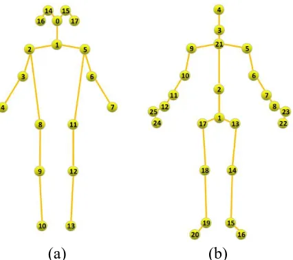
Fig. 3(a) shows the joint label of the Kinetics-skeleton dataset. The joint labels are: 0 nose, 1 262
neck, 2 right shoulder, 3 right elbow, 4 right wrist, 5 left shoulder, 6 left elbow, 7 left wrist, 8 263
right hip, 9 right knee, 10 right ankle, 11 left hip, 12 left knee, 13 left ankle, 14 right eye, 15 left 264
NTU-RGB+D32: NTU-RGB+D is the largest dataset with 3D joint annotations currently used 266
for human action recognition tasks. The dataset contains 60 action classes with a total of 56,000 267
action clips. All of these clips are performed by 40 volunteers in a constrained lab environment, 268
and captured by 3 cameras of the same height but from different horizontal angles: -45°, 0°, 269
45°32. The dataset provides the 3D joint location of each frame detected by the Kinect depth 270
sensor. There are 25 joints per subject in the skeleton sequence. Each clip is guaranteed to have a 271
maximum of 2 subjects. 272
273
[image:13.612.201.414.263.452.2]274
Fig. 3 The joint label of Kinetics-skeleton and NTU-RGB+D datasets. 275
The original paper of the NTU-RGB+D dataset recommended two benchmarks: 1) cross-276
subject (X-Sub) benchmark: The dataset in this benchmark is divided into a training set (40,320 277
clips) and a validation set (16,560 clips). The subjects in these two subsets are different; 2) cross-278
view (X-View) benchmark: The training set in this benchmark contains 37,920 clips captured by 279
cameras 2 and 3, and the validation set contains 18,960 clips captured by camera 132. We follow 280
this convention and report the top-1 recognition accuracy of the two benchmarks. 281
Fig. 3(b) shows the joint label of the NTU-RGB+D dataset. The joint labels are: 1 base of the 282
spine, 2 middle of the spine, 3 neck, 4 head, 5 left shoulder, 6 left elbow, 7 left wrist, 8 left hand, 283
9 right shoulder, 10 right elbow , 11 right wrist, 12 right hand, 13 left hip, 14 left knee, 15 left 284
ankle, 16 left foot, 17 right hip, 18 right knee, 19 right ankle, 20 right foot, 21 spine, 22 left hand 285
tip, 23 left hand Thumb, 24 right hand tip, 25 right thumb. 286
4.2 Effectiveness Analysis of AM-STGCN
287
In this section, we first conduct a lot of ablation experiments on the Kinetics-skeleton dataset: 1) 288
Adding attention block after the ConvS (spatial convolution) of different layers of the ST-GCN; 289
2) Adding multiple attention blocks after the ConvS of different layers; 3) Adding attention 290
blosks after ConvT (temporal convolution) of the layer; 4) Adding two other attention
291
mechanisms with different structures, CBAM29 and SENet30, to ST-GCN. Experiments are then 292
performed on NTU-RGB+D dataset to verify the generalization capabilities of the proposed 293
model AM-STGCN. 294
4.2.1 Baseline
295
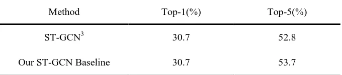
In order to evaluate the recognition performance of our improved model, we used baseline for 296
comparison experiments. Since our model is improved on the basis of the ST-GCN model, we 297
use the ST-GCN model as a baseline to analyze the advantages of AM-STGCN. We reproduced 298
the ST-GCN model on the Kinetics dataset based on the Ref. 3, and obtained very close results to 299
[image:14.612.137.477.579.654.2]the original paper (see Table 1). 300
Table 1 Baseline. 301
Method Top-1(%) Top-5(%)
ST-GCN3 30.7 52.8
4.2.2 Ablation experiment
[image:15.612.140.475.150.332.2]302
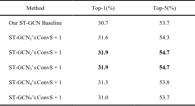
Table 2 The results of adding one attention block to the different layers of the ST-GCN. ST-GCN1's ConvS + 1 303
represents adding one attention block after the ConvS (spatial convolution) of the first layer of the ST-GCN. 304
Thereafter, Tables 3, 4, 5, and 6 have the same representation rules. 305
Method Top-1(%) Top-5(%)
Our ST-GCN Baseline 30.7 53.7
ST-GCN1’sConvS + 1 31.6 54.3
ST-GCN2’sConvS + 1 31.9 54.7
ST-GCN3’sConvS + 1 31.9 54.7
ST-GCN4’sConvS + 1 31.3 53.8
ST-GCN9’sConvS + 1 31.0 53.7
306
Table 2 shows the experimental results of adding one attention block after the ConvS (spatial 307
convolution) of different layers of the ST-GCN model. The results demonstrate that no matter 308
which layer we add an attention block to, the recognition accuracy always higher than the 309
baseline. The improvement of adding one attention block in the second and third layers is similar, 310
which can lead to ∼1.2% (on Top1) improvement over the baseline. The results of the remaining 311
[image:15.612.141.476.544.715.2]layers are slightly lower. 312
Table 3 The results of adding multiple attention blocks to different layers. 313
Method Top-1(%) Top-5(%)
Our ST-GCN Baseline 30.7 53.7
ST-GCN1’sConvS + 2 32.0 54.5
ST-GCN2’sConvS + 2 32.1 54.4
ST-GCN3’sConvS + 2 31.4 54.4
ST-GCN2’sConvS + 3 31.1 53.5
ST-GCN3’sConvS + 3 32.2 55.1
ST-GCN4’sConvS + 3 31.1 53.1
314
Table 3 shows the results of adding multiple attention blocks to different layers of the ST-315
GCN. It can be seen from Table 2 that adding one attention block to the first few layers of the 316
model is better than adding to the lower layer, so in the experiment of Table 3, we add two and 317
three attention blocks after the ConvS (spatial convolution) of the first few layers of ST-GCN. 318
Obviously, the results of adding multiple attention blocks after ConvS of a layer outperform 319
adding a single attention block, especially on ST-GCN3’s ConvS + 3, which can lead to 1.5% 320
(on Top1) and 1.4% (on Top5) improvement over the baseline. It demonstrates that more 321
attention blocks usually lead to better performance. We argue that multiple attention blocks can 322
reinforce the correlation information learned in the previous attention block, thus assigning each 323
[image:16.612.154.461.76.149.2]node a more appropriate weight. 324
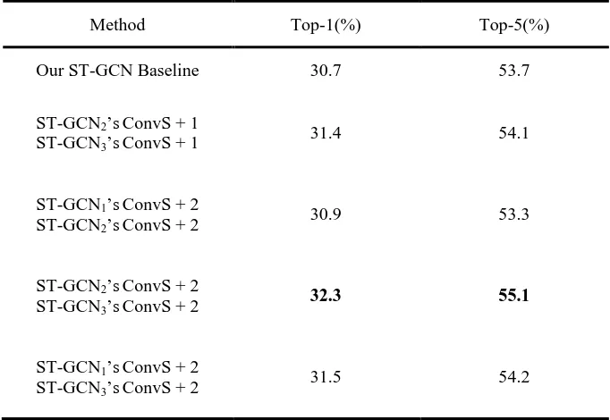
Table 4 The results of adding multiple attention blocks to multi-layers. 325
Method Top-1(%) Top-5(%)
Our ST-GCN Baseline 30.7 53.7
ST-GCN2’sConvS + 1
ST-GCN3’sConvS + 1 31.4 54.1
ST-GCN1’sConvS + 2
ST-GCN2’sConvS + 2
30.9 53.3
ST-GCN2’sConvS + 2
ST-GCN3’sConvS + 2 32.3 55.1
ST-GCN1’sConvS + 2
ST-GCN3’sConvS + 2 31.5 54.2
[image:16.612.135.476.464.699.2]Table 4 shows the results of adding multiple attention blocks to multi-layers of the ST-GCN 327
model. As shown in Tables 2, 3 and 4, we can find that only the third combination (ST-GCN2’s 328
ConvS + 2 & ST-GCN3’s ConvS + 2) improves accuracy compared to adding attention blocks to 329
single layer. The rest of the combinations do not improve accuracy compared to the individual 330
[image:17.612.136.480.235.363.2]structure in the combination. 331
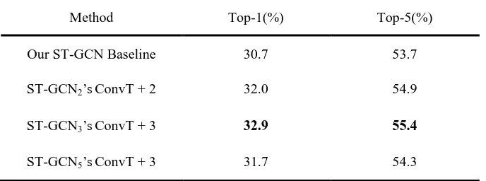
Table 5 The results of adding attention blocks after ConvT (temporal convolution) of one layer. 332
Method Top-1(%) Top-5(%)
Our ST-GCN Baseline 30.7 53.7
ST-GCN2’sConvT + 2 32.0 54.9
ST-GCN3’sConvT + 3 32.9 55.4
ST-GCN5’sConvT + 3 31.7 54.3
333
Table 5 shows the results of adding attention blocks after ConvT (temporal convolution) of 334
different layers of the ST-GCN model. Comparing the results of Table 3 and Table 5, we can 335
find that adding attention blocks after ConvT perform better than after ConvS. ST-GCN3’s 336
ConvT + 3 obtain the best improvement of adding attention blocks after ConvT, which 337
outperforms Our ST-GCN Baseline by 2.2% and 1.7% on Top1 and Top5 recognition accuracies; 338
ST-GCN3’s ConvS + 3 obtain the best improvement of adding attention blocks after ConvS, 339
which outperforms Our ST-GCN Baseline by 1.5% and 1.4% on Top1 and Top5 recognition 340
accuracies. One possible explanation is that ConvT has a bigger kernel size (9×1) and ConvS 341
has a small kernel size (1×1), thus ConvS is insufficient to capture precise spatial information. 342
Adding attention blocks after ConvT can learn the correlation of all nodes in all frames, while 343
adding attention blocks after ConvS can only learn the correlation of all nodes in one frame, thus 344
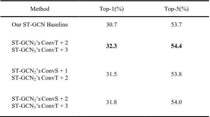
Table 6 The results of adding attention blocks after ConvT and ConvS of multi-layers. 346
Method Top-1(%) Top-5(%)
Our ST-GCN Baseline 30.7 53.7
ST-GCN2’sConvT + 2
ST-GCN3’sConvT + 3 32.3 54.4
ST-GCN2’sConvS + 1
ST-GCN2’sConvT + 2 31.5 53.8
ST-GCN2’sConvS + 2
ST-GCN3’sConvT + 3 31.8 54.0
347
Table 6 shows the results of adding attention blocks after ConvT and ConvS of multi-layers. 348
As shown in Tables 2, 3, 5 and 6, we can see that none of the combinations in Table 6 improves 349
accuracy compared to adding attention blocks to single layer. The results of Table 4 and 6 prove 350
that adding attention blocks to multiple layers does not further improve accuracy. 351
From Tables 2, 3, 4, 5 and 6, we find that adding attention blocks to the second and third 352
layer of ST-GCN can result in better performance. The possible reason is that the features 353
learned in these two layers are more consistent with the semantic representation of human 354
[image:18.612.136.478.533.636.2]motion. 355
Table 7 The results of adding CBAM and SENet to ST-GCN. 356
Method Top-1(%) Top-5(%)
ST-GCN+CBAM 31.9 54.3
ST-GCN+SENet 31.6 54.2
Our AM-STGCN 32.9 55.4
357
We selected two other attention mechanisms with different structures, CBAM29 and SENet30,
358
to be added to ST-GCN. CBAM contains spatial attention and channel attention, while SENet is
359
just channel attention. Table 7 shows the results of adding CBAM and SENet. As shown in
Table7, the results of our method are clearly better than those of the other two attention
361
structures, which prove that our attention mechanism is more suitable for ST-GCN.
362
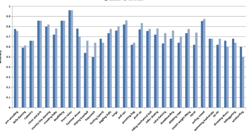
4.2.3 Further analysis on“Kinetics-Motion”
363
The authors of ST-GCN select a subset of 30 classes strongly related with body motions, named 364
as “Kinetics-Motion3”.For a detailed comparison, we further investigate the per-class differences 365
in accuracy on this subset. In Fig. 4, the horizontal axis is the action category of “Kinetics-366
Motion”, and the vertical axis is the accuracy of per-class. The dark blue represents Our ST-367
GCN Baseline and the light blue represents AM-STGCN, here AM-STGCN is the optimal 368
structure (i.e., ST-GCN3’s ConvT + 3) obtained after the analysis in the previous section. It can 369
be observed obviously that the accuracy of most actions get improved. Some classes even get 370
more than 10% improvement, such as hitting baseball, hopscotch, salsa dancing and squat. These 371
results also verify the superiority of our model for skeleton-based action recognition, in 372
particular on those classes strongly related with body motions. 373
[image:19.612.99.519.457.685.2]374
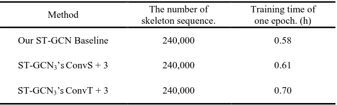
4.2.4 Time comparison on Kinetics
376
The Kinetics dataset provides a training set of 240,000 video clips, each clip contain 300 frames. 377
Every frame of the video clips is converted into a sequence of human skeletons represented by 378
coordinates through OpenPose34 toolbox. We compared the training time of one epoch of AM-379
STGCN model and our ST-GCN baseline on Kinetics dataset, and the results are shown in Table 380
8. ST-GCN3’s ConvS + 3 and ST-GCN3’s ConvT + 3, which performed better in the above
381
experiments, are selected to be compared with our GCN baseline. The training time of ST-382
GCN3’s ConvS + 3 and our ST-GCN baseline are similar, and ST-GCN3’s ConvT adds the 383
calculation in temporal dimension, so the training time is a little longer. These results 384
demonstrate that our AM-STGCN model do not add much time cost than ST-GCN model. 385
Table 8 The training time of AM-STGCN and ST-GCN methods. 386
Method The number of skeleton sequence.
Training time of one epoch. (h)
Our ST-GCN Baseline 240,000 0.58
ST-GCN3’sConvS + 3 240,000 0.61
ST-GCN3’sConvT + 3 240,000 0.70
387
4.2.5 Comparison with state-of-the-art methods
388
On Kinetics dataset, we compare AM-STGCN with “Feature Encoding”10, Deep LSTM32, 389
Temporal ConvNet14 and ST-GCN3 methods. Their recognition performance in terms of Top-1 390
and Top-5 accuracies are listed in Table 9. Obviously, our AM-STGCN with using attention 391
module outperforms ST-GCN by 2.2% and 2.6% on Top1 and Top5 recognition accuracies 392
respectively. It can be seen from Table 9 that our AM-STGCN is able to outperform previous 393
[image:20.612.137.477.380.486.2]Table 9 Comparison with the state-of-the-art on Kinetics dataset. 395
Method Date Top-1(%) Top-5(%)
Feature Encoding.10 2015 14.9 25.8
Deep LSTM32 2016 16.4 35.3
Temporal ConvNet14 2017 20.3 40.0
ST-GCN3 2018 30.7 52.8
Our ST-GCN Baseline - 30.7 53.7
Our AM-STGCN - 32.9 55.4
396
We found that most of the current skeleton-based action recognition studies are conducted on
397
RGB+D dataset, so we compare our method with state-of-the-art methods on
NTU-398
RGB+D dataset.
399
On NTU-RGB+D dataset, we compare AM-STGCN with Lie Group9, H-RNN11, Deep 400
LSTM32, VA-LSTM13, Temporal ConvNet14, Two-stream CNN16, HCN17, STA-LSTM12,
GCA-401
LSTM18, ARRN-LSTM20, MANs19, ST-GCN3, DPRL+GCNN26, SR-TSL22, PB-GCN24 and
402
AGCN23 methods. The results are shown in Table 10.
403
Comparisons with hand-craft feature based methods, CNN based methods and RNN 404
based methods. Table 10 shows that the performance of graph convolution based methods is 405
generally better than hand-craft feature based methods, CNN based methods and RNN based 406
methods. In particular, our AM-STGCN obtains very close results to HCN method on cross-407
view (X-View) benchmark, which performs best among CNN based methods. At the same time, 408
multi-person feature fusion is added in HCN, thus resulting in better performance on cross-409
subject (X-Sub) benchmark, but it also leads to the increase of computation. 410
Comparisons with other methods based on attention. We compare AM-STGCN with
411
other methods based on attention including STA-LSTM12, GCA-LSTM18, ARRN-LSTM20 and
[image:21.612.106.505.89.270.2]MANs19. From Table 10, we can see that our AM-STGCN is better than any other result except
413
for MANs under the X-View benchmark. MANs consists of Temporal Attention Recalibration
414
Module (TARM) and DenseNet-161, we can find that their baseline is higher than ST-GCN,
415
which may be due to DenseNet-161, because DenseNet-161 is much deeper and more complex
416
than ST-GCN. On X-View benchmark, our AM-STGCN outperforms ST-GCN by 3.1% and
417
MANs outperforms MANs (no attention) by 1.07%, which prove that our method can improve
418
the performance of the model more.
419
Comparisons with graph convolution based methods. 1) Single stream network. In Table
420
10,we can see clearly that our AM-STGCN with using attention module outperforms ST-GCN
421
by 1.9% and 3.1% on cross-view (X-View) benchmark and cross-subject (X-Sub) benchmark
422
respectively, which prove that our AM-STGCN model is equally effectiveness on NTU-RGB+D
423
dataset. Our AM-STGCN performs very close results to DPRL+GCNN on cross-subject (X-Sub)
424
benchmark and outperforms DPRL+GCNN by 1.6% on cross-view (X-View) benchmark in
425
Table 10. 2) Two-stream networks. The joint locations is the only input data of our AM-STGCN.
426
SR-TSL, PB-GCN and AGCN all have another form of input data as input to different streams,
427
thus forming a two-stream networks. SR-TSL(Position), PB-GCN(Jloc) and Js-AGCN are the
428
same as ST-GCN with only joint locations as input data. Among these methods, it can be seen
429
obviously form Table 10 that our AM-STGCN is superior to SR-TSL(Position) and
PB-430
GCN(Jloc) on both cross-subject (X-Sub) and cross-view (X-View) benchmark. In the paper of
431
AGCN, we find AGCN’s baseline is 92.7% on cross-view (X-View) benchmark, outperforms
432
ST-GCN by 4.4%, but Js-AGCN outperforms their baseline by only 1%. We think it may be that
433
different experimental environments cause different baselines. So in terms of relative increase in
434
accuracy, our method has achieved a good performance improvement. In addition, we have
added our attention module to Js-AGCN. In Table 10, the results of Js-AGCN+our attention
436
outperforms Our Js-AGCN Baseline by 0.5% and 0.4% on cross-view (X-View) benchmark and
437
cross-subject (X-Sub) benchmark respectively, which shows that our attention mechanism is also
438
effective on AGCN method, and proves that our method has certain robustness.
439
These results show our AM-STGCN model achieves a significant performance improvement. 440
Table 10 Comparison with the state-of-the-art on NTU-RGB+D dataset. 441
Method Date X-Sub(%) X-View(%)
Lie Group9 2014 50.1 52.8
H-RNN11 2015 59.1 64.0
Deep LSTM32 2016 60.7 67.3
Temporal ConvNet14 2017 74.3 83.1
VA-LSTM13 2017 79.4 87.6
Two-stream CNN16 2017 83.2 89.3
HCN17 2018 86.5 91.1
STA-LSTM12 2017 73.4 81.2
GCA-LSTM18 2017 74.4 82.8
ARRN-LSTM20 2019.04 81.8 89.6
MANs (no attention)19
2018
81.41 92.15
MANs19 83.01 93.22
ST-GCN3 2018 81.5 88.3
DPRL+GCNN26 2018 83.5 89.8
SR-TSL(Position)22
2018
78.8 88.2
SR-TSL(Velocity)22 82.2 90.6
[image:23.612.110.504.239.704.2]PB-GCN(Jloc)24
2018
82.8 90.3
PB-GCN(DR||DT)24 87.5 93.2
Js-AGCN23
2019.05
- 93.7
Bs-AGCN23 - 93.2
2s-AGCN23 88.5 95.1
Our Js-AGCN Baseline - 85.9 93.7
Js-AGCN + our attention - 86.4 94.1
Our AM-STGCN - 83.4 91.4
442
5 Conclusion 443
In this paper, we propose a new skeleton-based action recognition method called attention 444
module-based Spatial Temporal Graph Convolutional Networks(AM-STGCN), which can 445
overcome the weakness of ST-GCN model. In order to capture global information of skeleton 446
sequences, attention modules are added to learn the correlation information between all joints of 447
both spatial and temporal dimension. So AM-STGCN can extract long-range relationships from 448
input skeleton sequences, which improve the ability to model the dynamic change of human 449
body motions. Experiments on two large-scale action recognition datasets Kinetics and NTU-450
RGB+D achieve the better results, which indicate that AM-STGCN can effectively improve the 451
recognition accuracy. In future, we will improve our AM-STGCN in many possible directions, 452
such as improving attention modules or merging RGB modality. 453
Acknowledgments 455
This work is supported by the National Natural Science Foundation of China (Grant Nos. 456
61871182, 61302163), Hebei Province Natural Science Foundation (Grant Nos.F2015502062), 457
Hebei province science and technology support (Grant Nos.13210905). 458
459
References 460
1. H. Wang and C. Schmid, “Action recognition with improved trajectories,” in 2013 IEEE
461
International Conference on Computer Vision, pp. 3551-3558, IEEE, Sydney, NSW (2013)
462
[doi:10.1109/ICCV.2013.441].
463
2. H. Wang et al., “Dense trajectories and motion boundary descriptors for action recognition,” in
464
International journal of computer vision, 103(1), 60-79 (2013).
465
3. S. Yan, Y. Xiong, and D. Lin, “Spatial temporal graph convolutional networks for skeleton-based
466
action recognition,” in Thirty-Second AAAI Conference on Artificial Intelligence, pp. 7444-7452,
467
AAAI Press, New Orleans, Louisiana, USA (2018).
468
4. K. Simonyan, A. Zisserman, “Two-stream convolutional networks for action recognition in videos,”
469
in Advances in neural information processing systems, pp. 568-576 (2014).
470
5. C. Feichtenhofer, A. Pinz and A. Zisserman, “Convolutional two-Stream network fusion for video
471
action recognition,” in Proceedings of the IEEE Conference on Computer Vision and Pattern
472
Recognition, pp. 1933-1941, IEEE, Las Vegas, NV (2016) [doi:10.1109/CVPR.2016.213].
473
6. D. Tran et al., “Learning spatiotemporal features with 3D convolutional networks,”in 2015 IEEE
474
International Conference on Computer Vision, pp. 4489-4497, IEEE, Santiago (2015)
475
[doi:10.1109/ICCV.2015.510].
7. J. Carreira and A. Zisserman, “Quo Vadis, Action Recognition? A New Model and the Kinetics
477
Dataset,” in 2017 IEEE Conference on Computer Vision and Pattern Recognition, pp. 4724-4733,
478
IEEE, Honolulu, HI (2017) [doi:10.1109/CVPR.2017.502].
479
8. W. Du, Y. Wang and Y. Qiao, “RPAN: An end-to-end recurrent pose-attention network for action
480
recognition in videos,” in 2017 IEEE International Conference on Computer Vision, pp. 3745-3754,
481
IEEE, Venice (2017) [doi:10.1109/ICCV.2017.402].
482
9. R. Vemulapalli, F. Arrate, and R. Chellappa, “Human action recognition by representing 3d skeletons
483
as points in a lie group,” in Proceedings of the IEEE Conference on Computer Vision and Pattern
484
Recognition, pp. 588-595, IEEE, Columbus, OH (2014) [doi:10.1109/CVPR.2014.82].
485
10. B. Fernando et al., “Modeling video evolution for action recognition,” in Proceedings of the IEEE
486
Conference on Computer Vision and Pattern Recognition, pp. 5378-5387, IEEE, Boston, MA (2015)
487
[doi:10.1109/CVPR.2015.7299176].
488
11. Y. Du, W. Wang, and L. Wang, “Hierarchical recurrent neural network for skeleton based action
489
recognition,” in Proceedings of the IEEE Conference on Computer Vision and Pattern Recognition,
490
pp. 1110-1118, IEEE, Boston, MA (2015) [doi:10.1109/CVPR.2015.7298714].
491
12. S. Song et al., “An end-to-end spatio-temporal attention model for human action recognition from
492
skeleton data,” in Proceedings of the Thirty-First AAAI Conference on Artificial Intelligence, pp.
493
4263-4270, AAAI Press, San Francisco, California, USA (2017).
494
13. P. Zhang et al., “View adaptive recurrent neural networks for high performance human action
495
recognition from skeleton data,” in 2017 IEEE International Conference on Computer Vision, pp.
496
2136-2145, IEEE, Venice (2017) [doi:10.1109/ICCV.2017.233].
497
14. T. S. Kim and A. Reiter, “Interpretable 3d human action analysis with temporal convolutional
498
networks,” in IEEE Conference on Computer Vision and Pattern Recognition Workshops (CVPRW),
499
pp. 1623-1631, IEEE, Honolulu, HI (2017) [doi:10.1109/CVPRW.2017.207].
500
15. M. Liu, H. Liu, and C. Chen, “Enhanced skeleton visualization for view invariant human action
501
recognition,” in Pattern Recognition, 68, pp. 346-362, Elsevier (2017).
16. C. Li et al., “Skeleton-based action recognition with convolutional neural networks,” in 2017 IEEE
503
International Conference on Multimedia & Expo Workshops (ICMEW), pp. 597-600, IEEE, Hong
504
Kong (2017) [doi:10.1109/ICMEW.2017.8026285].
505
17. C. Li et al., “Co-occurrence feature learning from skeleton data for action recognition and detection
506
with hierarchical aggregation,” in Proceedings of the 27th International Joint Conference on
507
Artificial Intelligence, pp. 786-792, AAAI Press, Stockholm, Sweden (2018).
508
18. J. Liu et al., “Global Context-Aware Attention LSTM Networks for 3D Action Recognition,” in 2017
509
IEEE Conference on Computer Vision and Pattern Recognition (CVPR), pp. 3671-3680, IEEE, 510
Honolulu, HI (2017) [doi: 10.1109/CVPR.2017.391]. 511
19. C. Xie et al., “Memory attention networks for skeleton-based action recognition,” in Proceedings of
512
the 27th International Joint Conference on Artificial Intelligence, pp. 1639-1645, AAAI Press, 513
Stockholm, Sweden (2018). 514
20. W. Zheng et al., “Relational Network for Skeleton-Based Action Recognition,” arXiv preprint 515
arXiv:1805.02556v4, 2019. 516
21. C. Li et al., “ Spatio-temporal graph convolution for skeleton based action recognition,” in
Thirty-517
Second AAAI Conference on Artificial Intelligence, pp. 3482-3489, AAAI Press, New Orleans,
518
Louisiana, USA (2018).
519
22. C. Si et al., “Skeleton-based action recognition with spatial reasoning and temporal stack learning,” in
520
Proceedings of the European Conference on Computer Vision (ECCV), Lecture Notes in Computer
521
Science, vol 11205, pp. 106-121, Springer, Cham (2018) [
https://doi.org/10.1007/978-3-030-01246-522
5_7].
523
23. L. Shi et al., “Two-Stream Adaptive Graph Convolutional Networks for Skeleton-Based Action 524
Recognition,” in Proceedings of the IEEE Conference on Computer Vision and Pattern Recognition,
525
pp.12026-12035 (2019). 526
24. K. Thakkar, P J. Narayanan, “Part-based Graph Convolutional Network for Action Recognition,”
527
arXiv preprint arXiv:1809.04983, 2018.
25. X. Gao et al., “Optimized Skeleton-based Action Recognition via Sparsified Graph Regression,” 529
arXiv preprint arXiv:1811.12013v2, 2019. 530
26. Y. Tang et al., “Deep Progressive Reinforcement Learning for Skeleton-Based Action Recognition,” 531
in 2018 IEEE/CVF Conference on Computer Vision and Pattern Recognition, pp. 5323-5332, IEEE, 532
Salt Lake City, UT (2018) [doi: 10.1109/CVPR.2018.00558]. 533
27. X. Wang et al., “Non-local neural networks,” in Proceedings of the IEEE Conference on Computer
534
Vision and Pattern Recognition, pp. 7794-7803, IEEE, Salt Lake City, UT, USA (2018)
535
[doi:10.1109/CVPR.2018.00813].
536
28. Y. Du et al., “Interaction-Aware Spatio-Temporal Pyramid Attention Networks for Action
537
Classification,” in Proceedings of the European Conference on Computer Vision (ECCV), Lecture
538
Notes in Computer Science, vol 11220, pp. 388-404, Springer, Cham (2018)
539
[https://doi.org/10.1007/978-3-030-01270-0_23].
540
29. S. Woo et al., “CBAM: Convolutional Block Attention Module,” in Proceedings of the European
541
Conference on Computer Vision (ECCV), Lecture Notes in Computer Science, vol 11211, pp. 3-19,
542
Springer, Cham (2018) [https://doi.org/10.1007/978-3-030-01234-2_1].
543
30. J. Hu, L. Shen, and G. Sun, “Squeeze-and-Excitation Networks,” in 2018 IEEE/CVF Conference on
544
Computer Vision and Pattern Recognition, pp. 7132-7141, IEEE, Salt Lake City, UT (2018) 545
[doi:10.1109/CVPR.2018.00745]. 546
31. W. Kay et al., “The kinetics human action video dataset,” arXiv preprint arXiv:1705.06950, 2017.
547
32. A. Shahroudy et al., “NTU RGB+D: A large scale dataset for 3D human activity analysis,”
548
in Proceedings of the IEEE Conference on Computer Vision and Pattern Recognition, pp. 1010-1019,
549
IEEE, Las Vegas, NV (2016) [doi:10.1109/CVPR.2016.115].
550
33. K. He et al., “Deep residual learning for image recognition,” in Proceedings of the IEEE Conference
551
on Computer Vision and Pattern Recognition, pp. 770-778, IEEE, Las Vegas, NV (2016)
552
[doi:10.1109/CVPR.2016.90].
34. Z. Cao et al., “Realtime multi-person 2D pose estimation using part affinity fields,” in Proceedings
554
of the IEEE Conference on Computer Vision and Pattern Recognition, pp. 1302-1310, IEEE,
555
Honolulu, HI (2017) [doi:10.1109/CVPR.2017.143].
556 557
Yinghui Kong is a professor at North China Electric Power University, Baoding, China. She 558
received BS degree in Communication Engineering from Xidian University, Xian, China, in 559
1987, and MS degree in Power System & Its Automation from North China Electric Power 560
University, Beijing, China, in 1993, and PhD degree in Electrical Theory and New Techniques 561
from North China Electric Power University in 2009. Her research interests include deep 562
learning, computer vision, behavior recognition, expression recognition. 563
564 565
Caption List 566
567
Fig. 1 (a) Spatial-temporal graph of the skeleton and (b) Partitioning strategy, different colors 568
represent different subsets. 569
Fig. 2 The structure of AM-STGCN. 570
Fig. 3 The joint label of Kinetics-skeleton and NTU-RGB+D datasets. 571
Fig. 4 Category accuracies on the“Kinetics Motion”subset of the Kinetics dataset. 572
Table 1 Baseline. 573
Table 2 The results of adding a attention block to the different layers of the GCN. ST-574
GCN1’s ConvS + 1 represents adding one attention block after the ConvS of the first layer of the 575
ST-GCN. Thereafter, Tables 3, 4, 5, and 6 have the same representation rules. 576
Table 3 The results of adding multiple attention blocks to different layers. 577
Table 5 The results of adding attention blocks after ConvT of one layer. 579
Table 6 The results of adding attention blocks after ConvT and ConvS of multi-layer. 580
Table 7 The results of adding CBAM and SENet to ST-GCN.
581
Table 8 The training time of AM-STGCN and STGCN methods. 582
Table 9 Comparison with the state-of-the-art on Kinetics dataset. 583