Accepted Manuscript
Statistical inference in efficient production with bad inputs and outputs using latent prices and optimal directions
Scott E. Atkinson, Daniel Primont, Mike G. Tsionas
PII: S0304-4076(18)30016-2
DOI: https://doi.org/10.1016/j.jeconom.2017.12.009
Reference: ECONOM 4471
To appear in: Journal of Econometrics
Received date : 8 December 2016 Revised date : 13 July 2017 Accepted date : 3 December 2017
Please cite this article as: Atkinson S.E., Primont D., Tsionas M.G., Statistical inference in efficient production with bad inputs and outputs using latent prices and optimal directions.Journal of Econometrics(2018), https://doi.org/10.1016/j.jeconom.2017.12.009
STATISTICAL INFERENCE IN EFFICIENT PRODUCTION WITH BAD INPUTS AND OUTPUTS USING
LATENT PRICES AND OPTIMAL DIRECTIONS
Scott E. Atkinson Department of Economics
University of Georgia email: [email protected]∗
Daniel Primont Department of Economics
Southern Illinois University at Carbondale email: [email protected]
Mike G. Tsionas Department of Economics
Lancaster University Management School
& Athens University of Economics and Business, Athens, Greece LA1 4YX UK
email: [email protected]
January 23, 2018
Abstract
Researchers employ the directional distance function (DDF) to estimate multiple-input and multiple-output production, firm inefficiency, and productivity growth. We relax restrictive assumptions by computing optimal directions subject to profit maximization and cost minimization, correct for the potential endogeneity of inputs and outputs, estimate latent prices for bad outputs, measure firms’ responses to shadow prices rather than actual prices, and introduce an unobserved productiv-ity term into the DDF. For an unbalanced panel of U.S. electric utilities, a model assuming profit-maximization outperforms one assuming cost-minimization, while lagged productivity and energy price have the greatest effect on productivity.
JEL CODES: C11, C33, D24
KEY WORDS: Bayesian, directional distance, productivity, bad outputs, latent prices, efficiency, optimal directions, shadow prices
1
Introduction
As developed by Caves et al. (1982a, 1982b), the distance function (DF) has been
widely used to estimate radial representations of frontier production technologies where
firms employ multiple good inputs to produce multiple good outputs. The distance from
a production frontier is a measure of the firm’s technical efficiency (TE). The change
in this measure over time is efficiency change (EC), while the shift in the frontier over
time is technical change (TC). The sum of these two measures is productivity change
(PC). The DF is input- (output-) oriented if all inputs (outputs) are proportionally
scaled down (up) to reach the production frontier while all outputs (inputs) are held
constant.
One major shortcoming of the DF is that an entire set of inputs or an entire set of
outputs must be scaled by the same factor. This becomes problematic when modelling
the generation of electricity, since good inputs (capital, labor, and energy) and bad inputs
(such as sulfur) produce good outputs (residential and industrial/commercial electricity)
and bad outputs (pollutants). Using the DF, the researcher is not able to differentially
credit the firm for simultaneously reducing bad outputs while increasing good outputs.
In response, many authors have estimated an output DF and treated bad outputs like
good inputs (holding both constant). However, this does not credit the firm for reducing
bad outputs. Also, if bad inputs are consumed, no credit is given for their reduction.1
As an alternative, Chambers (1998) and Chambers et al. (1998) developed the
direc-tional distance function (DDF) which provides greater flexibility. It allows measurement
of unique additive changes in each input and output through the calculation of different
directions of movement for each to reach the production frontier. If non-zero directions
are used to change only inputs (outputs), the DDF is input- (output-) oriented. When
non-zero directions are used to change all inputs and outputs, the DDF is
technology-oriented.
Despite the greater flexibility of the DDF, researchers typically impose three
overly-restrictive assumptions. First, the researcher usually specifies arbitrary directions of
movement of current firm production toward the frontier to measure inefficiency.2
How-1A bad input like sulfur would be consumed only when it is organically bound to the coal and oil
which are burned to generate electricity. To our knowledge, only Yaisawarng and Klein (1994) include fuel sulfur content and sulfur dioxide emissions in a study of electric utility production.
2For example, assuming fixed directions, F¨are et al. (2005) estimate an output DDF for electric
ever, different directions of movement toward the frontier will generate different measures
of inefficiency. Three Data Envelopment Analysis (DEA) studies seek to avoid arbitrary
assignment of directions by using linear programming methods to choose directions that
maximize the measured distance (i.e., technical inefficiency) of the firm relative to a
DDF. The first, by F¨are et al. (2013), considers only good inputs and good outputs.
The second, by Hampf and Kr¨uger (2015), extends this analysis by including bad
out-puts. The stated goal of the third paper, by Zofio et al. (2013), is to compute optimal
directions consistent with a firm’s profit-maximization (PM) position on a DDF. They
assume that firms are currentlyprofit-maximizers and then measure the maximum
dis-tance from the current position. However, to measure the technology and productivity
at the PM position, one must estimate the DDF jointly with the first-order conditions
for PM. Since the latter are not included in their optimization model, the estimated
di-rections cannot be consistent with PM. In this paper we estimate these conditions jointly
with the DDF and compute directions consistent with PM, which we term “optimal-PM”
directions.
Our approach follows Chambers (1998), who formulates a PM problem which includes
a technology-oriented DDF (to measure the distance from the production frontier), and
derives the first-order price equations for good inputs and outputs. In order to compute
optimal-PM directions, Atkinson and Tsionas (2016) (AT) estimate the DDF jointly
with the first-order price equations for only good inputs and good outputs, since the
prices of bad outputs and bad inputs are missing. A complete set of utility-specific
pollution permit prices (shadow prices for bad outputs) for the years of our sample data
does not exist. As explained below, the prices of coal and oil include rebates for greater
amounts of the bad input, sulfur. However, data is not publicly available to compute an
hedonic price for sulfur.3 We generalize AT by assuming a data generating process for
latent prices of regulated bad outputs. These latent prices replace missing actual prices,
allowing us to add the first-order price equations for regulated bad outputs to the AT
system.
The second restrictive assumption of many DDF models is that all input and output
quantities are exogenous. Highly-influential papers by Olley and Pakes (1996) (OP) and
Levinsohn and Petrin (2003)(LP) consider the problem of estimating productivity in the
3In the more typical industry study, prices of all inputs are missing and our methodology can be
presence of endogenous inputs using panel data. Both papers estimate a single-output
Cobb-Douglas production function with a two-component random error term. The first
component is firm- and time-varying productivity that is unobserved by the
econome-trician but observed, at least in part, by the firm. Since the firm takes productivity
into account to some degree in choosing its inputs, endogeneity results. The second
random component is an idiosyncratic error that is assumed to be uncorrelated with
the explanatory variables and the productivity component. With the OP approach, the
econometrician proxies for the unobserved productivity component with a potentially
observable function. To obtain this function, OP first specify that investment is a
mono-tonic function of productivity for a given level of capital and vintage. They then invert
this function to obtain the productivity component as a proxy function of capital,
in-vestment, and vintage. Following OP, LP replace investment with materials and solve
for the productivity component as a proxy function of capital, materials, and vintage.
Productivity is assumed to follow a first-order Markov process. After discussing the
modification of OP and LP by Ackerberg, Caves, and Frazer (2015) (regarding when
the firm chooses labor), Wooldridge (2009) provides the exact set of moment conditions
required to identify each of these models, where instruments are subsets of current and
lagged inputs. However, as Griliches and Mairesse (1998) stress, if the econometrician
incorrectly specifies the productivity function, some degree of endogeneity remains. Both
OP and LP recognize the possible invalidity of their instruments as well as the typical
validity but unavailability of input and output prices as instruments.
In this paper, we avoid assuming that inputs are exogenous for electric utilities. In
our sample, they vary input choice over time and these choices are arguably correlated
with the idiosyncratic error term, when one misspecifies the proxy equation for
pro-ductivity. This results in the endogeneity of input quantities. Such a result potentially
applies to all input quantities with a cost-minimization (CM) model and to all input and
output quantities with a PM model. Instead, we utilize the prices of good inputs and
good outputs in our instrument set, since they are arguably exogenous. Utilities are price
takers in input markets, since these markets are national (due to trans-continental oil
and natural gas pipelines, trans-continental rail lines hauling coal and oil, and national
mobility of labor and capital). Regulated utilities, which comprise the vast majority
of our sample, face output prices that are set by regulatory commissions. The smaller
out-puts.4 Thus, for both types of firms, we employ input and output prices rather than
input quantities in our instrument set.
The third restrictive assumption with all previous DDF models is that actual prices
equal shadow (perceived) prices for the firm.5 If the two sets of prices differ, the
re-searcher must calculate optimal directions using shadow prices. Previous papers have
developed the methodology to estimate shadow prices for profit, cost, and distance
func-tions as summarized in Kumbhakar and Lovell (2000). However, our paper is the first
to estimate shadow prices using a DDF and the first-order price equations from PM. We
identify shadow prices by including input and firm-specific price inefficiency parameters
in these equations. These parameters are estimated jointly with optimal-PM directions.
In addition, this paper is the first to estimate a model free of these three restrictive
assumptions and, at the same time, explain the sources of firm productivity, without
resorting to inconsistent two-step methods. Typically the two steps are: 1) regress
output on a set of inputs and 2) regress the residuals on a set of explanatory variables that
were omitted from the first step. The two sets of variables must be uncorrelated to avoid
a potentially substantial bias.6 We avoid this improbable requirement by employing an
unrestricted profit function from which we derive productivity as an estimable function
of lagged productivity, profits, prices of inputs and outputs, vintage, and time. We
include this measure of productivity as an input in the DDF. This enables us to compute
the partial elasticities of productivity with respect to its arguments and decompose
productivity growth.
We apply our methodology to an unbalanced panel of U.S. electric utilities. This
sample significantly expands the AT data set by 80% to include years when a number
of utilities were restructured. We report posterior densities for optimal directions, TE,
EC, TC, PC, the resource implications of price inefficiency, and the sources of PC.
4The goal of deregulation was to increase competition, yielding greater TE, productivity growth, and
price efficiency. On the production frontier, the profit-maximizing firm achieves price efficiency when the price of each input equals the value of its marginal product. The cost-minimizing firm achieves allocative efficiency when ratios of input prices equal ratios of their marginal products.
5Reasons for deviations of shadow from actual prices include tax write-offs, rate-of-return regulation,
and constraints imposed by regulatory agencies or labor unions.
6See Wang and Schmidt (2002) for details on Monte Carlo experiments indicating substantial potential
2
The Directional Distance Function
2.1 Computing Optimal Directions
We assume a firm production technology that combines good inputs,
x = (x1, . . . , xN) ∈ RN+, and bad inputs, ˜x = (˜x1, . . . ,x˜J) ∈ RJ+, to produce good
outputs, y= (y1, . . . , yM)∈RM+, and bad outputs, ˜y= (˜y1, . . . ,y˜L)∈RL+. A firm with
vintage, τ, productivity shock, ω, at time t(t= 1, . . . , T),has production technology
T(ω, τ, t) ={(x,x˜,y,y˜;ω, τ, t) :x,x˜can producey,y˜with (ω, τ, t)}. (1)
Let g = (gx,gx˜,gy,gy˜) be a direction vector. Typically researchers assume that
(gx,gx˜,gy,gy˜) = (−1,−1,1,−1).Following Chambers (1998), we define the technology
DDF as
− →D
T(x,x˜,y,y˜;g, ω, τ, t)
= sup{β : (x+βgx,x˜+βgx˜,y+βgy,y˜+βgy˜)∈ T(ω, τ, t)}, (2)
That is, the typical assumption is that the analyst measures the distance from the frontier
using equal absolute values for directions which increase good outputs and reduce all
other inputs and outputs.
We now specify the important properties of the technology DDF that hold whether
directions are assigned or estimated optimally. As shown in Hudgins and Primont (2007),
for any values of the elements of g:
D1. Translation Property:
− →
DT(x+αgx,x˜+αgx˜,y+αgy,y˜+αgy˜;gx,gx˜,gy,gy˜, ω, τ, t)
=−→DT(x,x˜,y,y˜;g, ω, τ, t)−α, (3)
D2. g-Homogeneity of Degree Minus One:
− →D
T(x,˜x,y,y˜;λgx, λgx˜, λgy, λgy˜, ω, τ, t) =λ−1−→DT(x,˜x,y,y˜;g, ω, τ, t), λ >0, (4)
D3. Concavity:
− →
DT(x,x˜,y,y˜;g, ω, τ, t) is concave in (x,x˜,y,y˜;g, ω, τ, t), (5)
D4. Non-negativity:
− →
DT(x,x˜,y,y˜;g, ω, τ, t)≥0, (x,x˜,y,y˜;g, ω, τ, t)∈ T(ω, τ, t). (6)
Equation (3) says that the technology DDF will satisfy the translation property. For
will result in a decrease in the technology DDF by α. This is analogous to the property
of linear homogeneity with a Shephard distance function. Equation (4) indicates that
scaling each direction by λwill scale the technology DDF byλ−1. Equation (5) imposes
concavity of the technology DDF. Finally, equation (6) requires that the technology
DDF function be non-negative, which is easily imposed after estimation.
For the following properties we let “S” represent the assumption of strong
dispos-ability of all inputs and outputs:
D5–S. Good Input Monotonicity: We first assume that good inputs are strongly
disposable. In Appendix A.1 we show that this implies7
∂→−DT(x,x˜,y,y˜;g, ω, τ, t)/∂xn=0, n= 1, . . . , N. (7)
D6–S. Good Output Monotonicity: We assume that good outputs are strongly
disposable. Following the proof of D5-S, in Appendix A.2, we show that this assumption
implies
∂→−DT(x,x˜,y,y˜;g, ω, τ, t)/∂ym≤0, m= 1, . . . , M. (8)
Following the proof of D5–S, assuming that bad inputs are strongly disposable, we
can determine
D7–S. Bad Input Monotonicity:
∂−→DT(x,x˜,y,y˜;g, ω, τ, t)/∂x˜j ≥0, j= 1, . . . , J. (9)
Again following the proof of D5–S, assuming that bad outputs are strongly
dispos-able, we can determine
D8–S. Bad Output Monotonicity:
∂−→DT(x,x˜,y,y˜;g, ω, τ, t)/∂y˜l≥0, l= 1, . . . , L. (10)
However, researchers typically do not assume that bads are strongly disposable.
In-stead, most investigators maintain that bad inputs and bad outputs are weakly
dispos-able with good inputs and outputs. The weak disposability of bad inputs results from
their organic combination with good inputs, so that a reduction in bad inputs implies
a reduction in good inputs, outputs held constant. Likewise, bad outputs are weakly
disposable since to reduce them, we must divert resources from the production of good
outputs, holding inputs constant. Assuming weak disposability, we cannot determine
7The paper with all Appendices is stored at people.terry.uga.edu/directory/profile/atknsn/ and at
the global monotonicity property of bad inputs and bad outputs as in D7–S and D8–
S. However, as shown shortly, if we assume weak disposability, we can determine local
monotonicity conditions given that we also assume PM and know the signs of the prices
of bad inputs and bad outputs. If instead we assume CM, the firm is subject to only
the first-order conditions for inputs, so that the monotonicity conditions for good and
bad inputs are the same as with the PM model.
A number of studies have modeled electric utilities assuming PM. See Atkinson and
Halvorsen (1976, 1980) and Cowing (1978). Other researchers have assumed CM subject
to a set of regulatory constraints on earned rates of return and a requirement to satisfy
all demand at a given price (that is, output is taken as given). However, output may be
endogenous as with an ex ante cost function.8 Further, if these regulatory constraints
are not binding, utilities may maximize profits. Fowlie (2010) provides evidence of this
by showing that many regulated utilities earn allowed rates of return on capital that
considerably exceed the market rate of return, indicating that constraints on profits
may not be binding and output may be endogenous. These results indicate that a PM
model may be more appropriate than a CM model. Thus, we focus on the PM model
and compare the accuracy of its results to those of the CM model.
Temporarily suppressing all the arguments of −→DT(x,x˜,y,y˜;g, ω, τ, t), we follow
Chambers (1998) and assume that a firm maximizes profits, π, by choosing values of
x,y,x˜,y˜ to solve
sup{py(y+−→DTgy)−p˜y(˜y+−→DTg˜y)−px(x+−→DTgx)−p˜x(˜x+−→DTg˜x) }
, (11)
where py ≥ 0,p˜y ≥ 0,px ≥0, and p˜x ≤ 0 are price vectors and the econometrician
either pre-determines or estimates g. Further, we definep= (py,p˜y,px,px).˜
Typically (as indicated above) the DDF is estimated without the first-order
condi-tions for PM, where one has assumed a set ofa priorifixed directions. However, in this
paper we assume that the firm chooses (x,x˜,y,y˜) subject to the first-order conditions
for PM and we estimate optimal-PM directions consistent with these conditions.9 The
8See Pope and Just (1996) regarding identification and estimation of an ex ante cost function. 9The CM model is obtained by using only the first-order conditions for input prices and assuming
first-order conditions are:
pn/ϱ(p,g) = ∂−→DT(x,x˜,y,y˜;g, ω, τ, t)/∂xn, n= 1, . . . , N, (12)
pm/ϱ(p,g) = −∂−→DT(x,x˜,y,y˜;g, ω, τ, t)/∂ym, m= 1, . . . , M, (13)
pj/ϱ(p,g) = ∂−→DT(x,x˜,y,y˜;g, ω, τ, t)/∂x˜j, j = 1, . . . , J, (14)
pl/ϱ(p,g) = ∂−→DT(x,x˜,y,y˜;g, ω, τ, t)/∂y˜l, l= 1, . . . , L, (15)
where
ϱ(p,g) =[∑
m
pmgm− ∑
n
pngn− ∑
j
pjgj− ∑
l plgl
]
. (16)
We assume that ϱ(p,g) > 0, where ϱ(p,g) is the optimal value of the Lagrangian
multiplier, which is the change in profits due to a small improvement in the production
technology. For details see Hudgins and Primont (2007) who show that one can solve
the profit-maximization problem in (11) or solve the equivalent Lagrangian function
L=pyy−pxx−p˜yy˜−p˜xx˜+ϱ−→DT(x,x˜,y,y˜;g, ω, τ, t), (17)
in order to obtain this interpretation of ϱ.
All prices are assumed to be non-negative except for the price of bad inputs, which is
non-positive. The prices of good outputs and the prices of good inputs are non-negative
by definition. The price of bad outputs is positive, since the firm must pay a fine or
buy emission permits for additional production of bad outputs. When a bad input is
organically bound to a good input, the price of the bad input is negative, since the firm
must be compensated for utilizing it.
For the following two properties, “W” indicates weakly disposable. Assuming weak
disposability of bad inputs and thatpx˜≤0, from (14) we obtain locally:
D7–W. Bad Input Monotonicity:
∂−→DT(x,x˜,y,y˜;g, ω, τ, t)/∂x˜j ≤0, j= 1, . . . , J. (18)
Assuming weak disposability of bad outputs and that py˜ ≥ 0 from (15) we obtain
locally:
D8–W. Bad Output Monotonicity:
∂−→DT(x,x˜,y,y˜;g, ω, τ, t)/∂y˜l≥0, l= 1, . . . , L. (19)
In this manner we maintain PM and use assumptions about the prices of bad inputs
and bad outputs to locally restrict the range of the partial derivatives in D7–W and
D8–W. For the CM model, only the monotonicity conditions for good and bad inputs
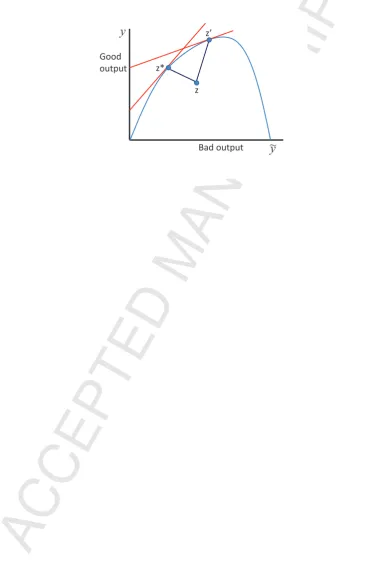
Rather than assume fixed directions, in this paper we compute optimal directions
that are consistent with PM and CM. In Fig. 1, a firm increases a good output and
reduces a bad output by moving from z to z∗, the PM point. This is consistent with
the traditional assumptions, where the directions for the good output and bad output
are positive and negative, respectively. However, the signs of optimal directions may
be quite different. In Fig. 1, if a firm moved from z to the point of PM at z′, from
(2) the directions (gy,gy˜) are both positive since the good output and the bad output
would both increase. One can easily substitute ˜xor xfor ˜yand obtain similar results.
An electric utility subject to the first-order conditions for PM may maximize profits by
increasing good outputs, increasing some inputs to produce the additional good outputs,
decreasing regulated bad outputs, and increasing unregulated bad outputs due to the
increase in good outputs. Thus, we impose no a priori sign restrictions on the optimal
direction of any input or output.
The input and output DDF are easily obtained as special cases of the technology
DDF. The output DDF changes good and bad outputs in the direction (0,0,gy,g˜y), for
a given level of inputs in order to move to the frontier of T(ω, τ, t). The input DDF
changes good and bad inputs in the direction (gx,g˜x,0,0), for a given level of good and
bad outputs in order to move to the frontier of T(ω, τ, t).
3
Econometric Formulation
3.1 The Technology Directional Distance System and the Translation
Restrictions
Assume that we have panel data for firmi(i= 1, . . . ,N) in time periodt(t= 1, . . . , T)
on all inputs and outputs. We then formulate our technology DDF as a quadratic
function of x,x˜,y,y˜, τ, andt as:
− →
DT(xit,x˜it,yit,y˜it;τit, t) = N ∑
n=1
γn(xn,it) + M ∑
m=1
γm(ym,it) + J ∑
j=1
γj(˜xj,it) + L ∑
l=1
γl(˜yl,it)
+ 1 2 N ∑ n=1 N ∑
n′=1
γnn′(xn,it)(xn′,it) +
1 2 J ∑ j=1 J ∑
j′=1
γjj′(˜xj,it)(˜xj′,it)
+ 1 2 M ∑ m=1 M ∑
m′=1
γmm′(ym,it)(ym′,it) +
1 2 L ∑ l=1 L ∑
l′=1
+ J ∑ j=1 N ∑ n=1
γjn(˜xj,it)(xn,it) + M ∑ m=1 N ∑ n=1
γmn(ym,it)(xn,it)
+ L ∑ l=1 N ∑ n=1
γln(˜yl,it)(xn,it) + M ∑ m=1 J ∑ j=1
γjm(ym,it)(˜xj,it)
+ L ∑ l=1 J ∑ j=1
γjl(˜yl,it)(˜xj,it) + L ∑ l=1 M ∑ m=1
γlm(˜yl,it)(ym,it)
+
N ∑
n=1
γnt(xn,it)dt+ M ∑
m=1
γmt(ym,it)dt+ J ∑
j=1
γjt(˜xj,it)dt
+
L ∑
l=1
γlt(˜yl,it)dt +
T ∑ t=1 γtdt+ N ∑ n=1
γnτ(xn,it)τit
+
M ∑
m=1
γmτ(ym,it)τit+ J ∑
j=1
γjτ(˜xj,it)τit
+
L ∑
l=1
γlτ(˜yl,it)τit +γττit, (20)
wheredtis a year dummy. We later accept the null thatdtandτitenter (20) linearly using
a likelihood ratio test at the .05 level. Hence, we drop all interaction terms involving
these variables from this equation.10
We can now restate the first-order conditions for PM, (12)-(15), in terms of the
parameters of the quadratic DDF for each good input price equation as
pn,it/ϱ=γn+ N ∑
n′=1
γnn′(xn′,it) + J ∑
j=1
γjn(˜xj,it) + M ∑
m=1
γmn(ym,it)
+
L ∑
l=1
γln(˜yl,it), (21)
for each good output price equation as
pm,it/ϱ=− [
γm+ M ∑
m′=1
γmm′(ym′,it) + J ∑
j=1
γjm(˜xj,it) + N ∑
n=1
γmn(xn,it)
+
L ∑
l=1
γlm(˜yl,it) ]
, (22)
for each bad input price equation as
pj,it/ϱ=γj+ J ∑
j′=1
γjj′(˜xj′,it) + N ∑
n=1
γjn(xn,it) + M ∑
m=1
γjm(ym,it)
10F¨are and Lundberg (2005) prove that only two functional forms have a second-order Taylor series
+
L ∑
l=1
γjl(˜yl,it), (23)
and for each bad output price equation as
pl,it/ϱ=γl+ L ∑
l′=1
γll′(˜yl′,it) + J ∑
j=1
γjl(˜xj,it) + N ∑
n=1
γln(xn,it)
+
M ∑
m=1
γlm(ym,it). (24)
The restrictions guaranteeing the translation property in (3) are imposed
paramet-rically on (20) and on (21)-(24).11 To derive these restrictions for an input, an output,
and a technology DDF, we generalize Hudgins and Primont (2007) by adding bad inputs
and bad outputs. To simplify notation, let ˜z= (x,x˜,y,y˜).First, assuming a quadratic
functional form for the technology DDF:
− → DT(˜z) =
W ∑
w=1
γwzw˜ +
W ∑
w=1
W ∑
w′=1
γww′zw˜ z˜w′, (25)
where w= 1, . . . , W, W =M +N +J +L. To determine the appropriate parametric
restrictions that guarantee the translation property incorporating g, we note that the
translation property requires that
− →
DT(˜z+αg;g) =
W ∑
w=1
γw(˜zw+αgw)
+ W ∑ w=1 W ∑
w′=1
γww′(˜zw+αgw)(˜zw′ +αgw′)
=
W ∑
w=1
γwz˜w+ W ∑
w=1
W ∑
w′=1
γww′z˜wz˜w′−α. (26)
3.2 The Stochastic Framework with Shadow and Latent Prices
3.2.1 Stochastically Imposing the Translation Property Restrictions
Generalizing Hudgins and Primont (2007), we derive the following parametric
re-strictions to stochastically impose the translation property in (26) for the technology
11An alternative to the quadratic is the logarithmic transcendental technology translation function
DDF:
M ∑
m=1
γmgm+ L ∑
l=1
γlgl+ N ∑
n=1
γngn+ J ∑
j=1
γjgj =ϑo,
M ∑
m=1
γmn′gm+ L ∑
l=1
γln′gl+ N ∑
n=1
γnn′gn+ J ∑
j=1
γjn′gj =ϑ, ∀n′,
M ∑
m=1
γmm′gm+ L ∑
l=1
γlm′gl+ N ∑
n=1
γm′ngn+ J ∑
j=1
γjm′gj =ϑ, ∀m′, (27)
M ∑
m=1
γj′mgm+ L ∑
l=1
γj′l′gl+ N ∑
n=1
γj′ngn+ J ∑
j=1
γjj′gj =ϑ, ∀j′,
M ∑
m=1
γl′mgm+ L ∑
l=1
γll′gl+ N ∑
n=1
γl′ngn+ J ∑
j=1
γjl′gj =ϑ, ∀l′,
where ϑo ∼ N (−1, c2) and ϑ ∼N (0, c2),N is the normal density, and c = 10−4 to keep the variance small around zero. The stochastic restrictions in (27) are, in fact,
semi-informative priorsplaced upongandγ, a vector of allγwparameters. These parameters
are estimated jointly, as explained below. In a more traditional, non-Bayesian approach,
one would set ϑo =−1, ϑ= 0.
To obtain the corresponding restrictions for the input and output DDF models,
simply eliminate the summation terms for the outputs and the inputs, respectively. For
the technology DDF model, we have imposed symmetry for all the double-subscripted
coefficients for all inputs and outputs. Note that the introduction of parameters to
measure the direction for each input and output occurs only through the translation
property restrictions.
3.2.2 Modeling ω
Assuming now that production is a function of inputs, outputs, vintage and a
Hicks-neutral productivity shock, ω, the resulting profit function obtained from (11) is
π=π(py,p˜y,px,px˜, ω;g, τ, t) =π(p, ω;g, τ, t). (28)
By definition, πis non-decreasing, monotonic inω. Strengthening this condition to
posi-tive monotonicity ofπinω, we can write the inverse function forωasω =f(p, π;g, τ, t).
0 =−→DT(x,x˜,y,y˜;g, τ, t) +vit+ωit−uit, (29)
where the stochastic part is comprised of an idiosyncratic i.i.d. term,vit, which has zero
mean,ωit, and a one-sided component,uit. Whilevitreflects errors in optimization due to
random events beyond the control of the firm (such as weather),uit reflects firm-specific
inefficiencies that may vary over time. We generalize the productivity component, ωit,
by including ωi,t−1, which is lagged ωit,and utilizing p∗it, where the star indicates that
latent prices replace missing prices:
ωit=f(ωi,t−1,p∗it, πit;g, τit, t) +εit,1 (30)
and we must obtain an approximation to the unknown functional form f(·). We further
specify that
log(uit) =γ1+γ2ωit+γ3ωi,t−1+γ4logui,t−1+γ5t+d′itγo+Z′i,t−1δ+εit,2, (31)
where dit denotes firm dummies, and Zi,t−1 contains lagged values of all inputs and
outputs.
We now consider different approximations of (30). To obtain a
translog-neural-network approximation, let zit= (ωi,t−1,p∗it, πit;g, τit, t). Then
f(zit) =ao+a′zit+12z′itAzit+ G ∑
g=1
λgφ (
z′itbg )
, (32)
where the activation functionφ(κ) = 1+exp(1 −κ),−∞< κ <∞. As a second alternative,
we use a second-order approximation:
f(zit) =ao+a′zit+12z′itAzit. (33)
As a third alternative, we use the Fourier approximation:
f(zit) =ao+a′zit+ 12z′itAzit+ ∑Φ
ϕ=1 {
u0ϕ+ 2∑Jℓ=1 (
uℓϕcos(ℓk′ϕzit) +vℓϕsin(ℓk′ϕzit) )}
, (34)
where kϕis a multi-index, Φ is a number determined by dim(zit),J is the order of the
expansion, and u0ϕ, uℓϕ, vℓϕare unknown parameters. The multi-indices are constructed
using the following rules: i) the zero vector and any kϕ whose first non-zero element
is negative are deleted; ii) Every index with a common integer divisor is also deleted.
Gallant (1982) shows that A = −∑Φϕ=1u0ϕkϕk′ϕ. Notice that we can leave A
unre-stricted and obtain a different Fourier approximation. We use the same re-scaling as in
Gallant (1982) and Feng and Serletis (2009) with the exception that we do not use logs.
be achieved through a common scale in zit. Finally, we can employ a full third-order
approximation:
f(zit) =ao+ b ∑
i=1
aizit+ b ∑
i=1
b ∑
j=1,i≤j
bijzitzjt+ b ∑ i=1 b ∑ j=1 b ∑
k=1,i≤j≤k
cijkzitzjtzkt, (35)
where bis the number of elements in zit.
We perform posterior analysis with all these specifications, which are flexible enough
to cover nearly every empirical case. For any model with parameters θ ∈ Θ ⊆ Rdθ,
including any latent variables in the model, denote the prior by p(θ), the likelihood by
L(θ;Y) for dataY and the posterior byp(θ|Y). We know
p(θ|Y) = L(θ;Y)p(θ)
p(Y) , (36)
where the marginal likelihood is
p(Y) = ∫
ΘL
(θ;Y)p(θ)dθ. (37)
For two different models, say 1 and 2, we define the Bayes factor in favor of model 1 and
against model 2 as:
BF1:2= p1(Y)
p2(Y)
. (38)
The Bayes factors, in our application, are reported in Table 2. These results clearly favor
the third-order approximation in (35). All of our results will, therefore, be conditional
on the selection of this functional form for the productivity equation.
The computation of the marginal likelihood is an involved operation. Here, we
compute it using the importance sampling techniques in Perrakis, Ntzoufras and Tsionas
(2014).
We also treat firm-specific directions,gi, as latent variables and assume the following
prior:
gi ∼NN+M+J+L(¯g,Σg), (39)
where ¯gdenotes the prior mean vector whose elements consist of reasonable prior beliefs
(namely, -1 for all inputs and the bad outputs and +1 for the good outputs) and Σg is
constructed so as to reflect reasonable deviations from these prior beliefs. Below we find
that the posteriors are highly insensitive to variations in these priors.
Having estimated productivity (ωit), we compute PC = ∂ω∂tit and EC = ∂u∂tit, using
equations (30) and (31). Then TC = PC−EC. For more details on computing these
quantities, see Grosskopf (2003). We also compute returns to scale (RTS) as the sum of
3.2.3 Shadow Prices
To incorporate shadow prices as the relevant prices for the firm we write:
ps n ϱs =
∂−→DT (z;g)
∂xn , n= 1, ..., N, (40)
psm ϱs =−
∂−→DT (z;g)
∂ym
, m= 1, ..., M, (41)
ps j ϱs =
∂−→DT (z;g)
∂x˜j
, j= 1, ..., J, (42)
psl ϱs =
∂−→DT (z;g)
∂y˜l
, l= 1, ..., L, (43)
with ϱs =∑Mm=1psmgm−∑Nn=1psngn− ∑J
j=1psjgj− ∑L
l=1pslgl, where the superscript s
denotes shadow (or perceived) prices to the firm. The shadow prices satisfy the
first-order conditions, which are used to complete the system, since we have many endogenous
variables but only one DDF equation. Shadow prices are the relevant prices for the
shadow-profit-maximizing firm. Actual prices potentially differ from shadow prices by
an amount ξq, q=n, m, j, l:
psn=pn+ξn, n= 1, ..., N, (44)
psm =pm+ξm, m= 1, ..., M, (45)
psj =pj +ξj, j= 1, ..., J, (46)
psl =pl+ξl, l= 1, ..., L. (47)
The variableξit is latent, where we assume the following prior:
ξit= [ξ′N,ξM′ ,ξ′J,ξ′L]′ ∼NN+M+J+L(0,Ω), (48)
where ξN = [ξn,it, n = 1, ..., N]′, ξM = [ξm,it, m = 1, ..., M]′, ξJ = [ξj,it, j = 1, ..., J]′,
ξL= [ξl,it, l= 1, ..., L]′, and whereΩis unknown.
error terms vq, q=n, m, j, l, as:
pn=ϱs(p, g, ξ)·∂ ⃗DT(z;g) ∂xn −
ξn+vn, n= 1, . . . , N, (49)
pm=−ϱs(p, g, ξ)·
∂ ⃗DT(z;g)
∂ym −
ξm+vm, m= 1, . . . , M, (50)
pj =ϱs(p, g, ξ)·
∂ ⃗DT(z;g)
∂xj˜ −ξj+vj, j = 1, . . . , J, (51)
pl=ϱs(p, g, ξ)·
∂ ⃗DT(z;g)
∂y˜l −
ξl+vl, l= 1, . . . , L, (52)
where ϱs(p, g, ξ)=(ϱ(p, g) +∑Mm=1ξmgm−∑nN=1ξngn−∑Jj=1ξjgj −∑Ll=1ξlgl )
, the
vectorξ= (ξN,ξM,ξJ,ξL), and the vectorp= (pN,pM,pJ,pL). We can normalize the
first element of ξN to zero, since we can only identify relative price distortions.12
Assuming that we have data on prices for all inputs and outputs, estimating all of the
normalized price equations in (12)–(15) together with the DDF would generate a
singu-larity in the covariance matrix of the residuals. This occurs since the normalized price
equations sum to 1 for any value ofg (as is seen from adding (12)-(15) with appropriate
changes in sign and comparing to (16) ). The choice of which price equation to drop
does not impact the results. The technology system is the DDF in (20) substituted into
(29) and N+M+J+L−1 of the price equations in (49)–(52), subject to imposition of
the restrictions in (27). Relative to one normalized input or output efficiency parameter,
we can estimate both input and output price efficiencies by estimating this system, since
all the price equations are included.
3.2.4 Completing the System using Reduced-Form Equations
Assume now a worse-case scenario where we lack prices and alternative valid
instru-ments for the endogenous bads, ˜x and ˜y, so that we are unable to identify the DDF
using equations like (51) and (52). Assume further that we are unable to generate latent
prices for ˜xand ˜y. We can still identify the technology DDF. First we create a system of
equations consisting of (20) substituted into (29) andN+M−1 of the price equations
in (49) and (50), subject to the restrictions in (27). Then we complete this system by
including reduced-form equations for ˜x and ˜y following standard LIML practices as in
12This occurs since PM means that the firm chooses absolute levels of outputs given CM, which
Pagan (1979). The input and output DDF systems would be constructed analogously.
The explanatory variables for these equations are prices of the good inputs and good
outputs, firm dummies, and time dummies. See Appendix B for further details.
3.2.5 Completing the System using Latent-Price Equations
Frequently, actual prices for inputs and outputs are missing. With rare exceptions,
prices for good inputs are confidential for privately-owned, unregulated firms. While data
on prices and quantities of good inputs and outputs are typically reported by regulated
electric utilities, the federal government currently allows many utilities to redact data on
wages. Publicly-available data sources intermittently report prices from thin tradable
permit markets for the regulated bad outputs that we examine, sulfur dioxide (SO2)
and nitrogen oxide (NOx). No reliable prices exist for the unregulated pollutant that we
model, carbon dioxide (CO2). Further, prices of bad inputs are missing for all firms. In
theory one could estimate prices for sulfur, a bad input, which is chemically bound to
coal and oil, which are good fuel inputs. However, this would require the use of hedonic
methods, which are infeasible due to data confidentiality.13
In place of missing actual prices, we can sample prices from their conditional
poste-riors generated by their FOCs to generate latent pricesp∗j andp∗l for ˜xand ˜yto replace
the missing pj and pl in (51) and (52), respectively. Then we can estimate a complete
(fully-identified) system comprised of (20) substituted into (29) and (49)–(52), subject
to (27).14
Assuming that input prices are unobserved and, therefore, generated as latent
vari-ables requires stochastic assumptions. Of course, these assumptions have to be consistent
with what is known about the sector under study and the nature of sectoral input prices.
Let p∗ = [p∗l, l = 1, . . . , L;p∗j, j = 1, . . . , J]. Assume there is a Q ×1 vector of
predetermined variables fit, so that E(p∗it,h|fit, ζh) = fit′ζh for h = 1, . . . , J +L where
13In a competitive market, the delivered price of coal is a function of the Btu/ton, the percent
sul-fur/ton, and transportation charges. Given this information, a hedonic regression would yield the implicit price of the percent sulfur/ton. Unfortunately, the DOE publishes data on all these variables except for transportation charges, which are confidential. A way around this would be to obtain data on the mine-mouth price/ton, which could be regressed on Btu/ton and percent sulfur/ton. Again unfortunately, complete mine-mouth data on price/ton linked to a specific mine and utility is confidential.
14One can apply this approach if prices are also missing for elements ofxandyby simply generalizing
ζh, h= 1, . . . , J +L areQ×1 parameter vectors. Define Fit=IJ+L⊗fit so that
p∗it=Fitζ+ϵit, ϵit ∼NJ+L(0,Σp∗). (53)
Thus, the predetermined variables are in Fit.
This can be written in the standard multivariate regression form asp∗=Fζ+ϵ. For
a particular observation we assume
p∗it|Fit, ζ ∼NJ+L(Fitζ,Σp∗), (54)
where ζ = [ζ1′, . . . , ζJ′+L]′ is Q′ ×1 where Q′ = (J +L)Q. As we lack specific prior
information, we assume:
p(ζ,Σp∗)∝fN,J+L(ζ; ¯ζ,V¯ζ)· |Σp∗|−(J+L+1)/2, (55)
wherefN,J+L(ζ; ¯ζ,V¯ζ) denotes a (J+L)−dimensional normal density with mean vector
¯
ζ = 0J+L and covariance ¯Vζ = 104IJ+L. Relative to the previous approach, we now
have to draw from three additional conditional posterior distributions, viz.:
p∗|ζ,Σp∗, . . . ,
ζ|p∗,Σp∗, . . . ,
Σp∗|p∗, ζ, . . . .
(56)
All three additional conditional posterior distributions are in standard form.
Stan-dard results yield the following:
ζ|· ∼NQ′(ˆζ,Vˆ), (57)
where ˆζ = (F′(I⊗Σ−p∗1)−1F )−1
F′(I⊗Σp−∗1)−1p∗ and ˆV = (
F′(I⊗Σ−p∗1)−1F )−1
. For
the covariance matrix we have:
p(Σp∗|·)∝ |Σp∗|−(nT+J+L+1)/2exp (
−tr ¯AΣ−p∗1 )
, (58)
where ¯A= (p∗−Fζ)′(p∗−Fζ).
Assuming the covariance matrix of errors in (51) and (52) is ˜Σ we obtain that
p∗it|· ∼NJ+L(¯pit,V¯p∗), (59)
where ¯pit = (Σ−p∗1 + ˜Σ−1)−1(Σ−p∗1Fitζ+ ˜Σ−1G˜it) and ¯Vp∗ = (Σp−∗1+ ˜Σ−1)−1, where G˜it
denotes the RHS of (51) and (52).15
15Coupled with (27), the price equations in (49)–(52) satisfy the order condition for identification.
3.3 Measurement of Allocative Inefficiency and its Resource Implica-tions
Using (49)–(52) we can measure allocative inefficiency (AI) as the sum of the error
in each input price equation times its corresponding quantity plus the sum of the error
in each output price times its corresponding quantity all divided by ϱ(p, g) (defined in
(16)):
AIit=
N ∑
n=1
ξn,itxn,it+ M ∑
m=1
ξm,itym,it+ J ∑
j=1
ξj,itx˜j,it+ L ∑
l=1
ξl,ity˜l,it
/ϱ(p, g). (60)
To reiterate, this measure depends on the errors from (49)–(52) weighted by
corre-sponding quantities. Since we interpret ϱ as the change in profits due to an incremental
improvement in the production technology, we can decompose ϱ into two parts: that
due to reducing price inefficiency and that due to reducing technical inefficiency. The
numerator of AIit is the former component.
To account for parameter uncertainty,AIit is averaged across Markov Chain Monte
Carlo (MCMC) draws in standard Rao-Blackwell fashion. For each MCMC draw, AIit
in (60) can be transformed as AIfit := AIit−min{AIit}. Allocative efficiency (AE) is
then computed as
AEit = 100−AIfit. (61)
Since we make this computation for each MCMC draw, the probability of any one firm
being fully efficient is very small. Our procedure allows us to resolve the standard
problem of relative efficiency estimation by using our variant of the corrected ordinary
least-squares technique in a Bayesian framework.
We also compute the estimated percent change in input usage for inputs and outputs
due to the firm producing at profit-maximizing levels based on market prices rather than
profit-maximizing levels based on shadow prices. For each of equations (49)–(52) we
solve the linear system for each draw of parameters and latent variables, which include
the estimated value of ξ. A solution zs∗,o is obtained for iteration s, s = 1, . . . , S, for
all observations o = 1, ...,NT. This measures the optimal level of inputs subject to
market prices, since the solved equations are in terms of these prices. The amounts z
are the current optimal amounts of input usage subject to shadow prices. Then we take
the Monte Carlo average z∗,o = S−1∑Ss=1zs∗,o to account for parameter uncertainty.
3.4 Posterior Predictive Measure of Cost-Minimization versus Profit Maximization
As indicated above, one can obtain the CM model by estimating the DDF with only
the good and bad input price equations. This entails estimation of (20) substituted into
(29), (49), and (51), where (27) is imposed during our MCMC iterations.
We wish to be able to compare the CM model to the PM model in terms of their
predictive abilities. Suppose all T observations (say yi ∈ ℜT ) of a certain utility
i ∈ {1, . . . ,N } are omitted from the dataset Y so the new dataset is Y−i. The new
posterior is p(θ(i)|Y−i) and the posterior predictive distribution for the ith utility is:
p(˜yi|Y−i) = ∫
p(˜yi|θ(i), Y−i)p(θ(i)|Y−i)dθ(i). (62)
We are interested in the posterior distribution of the absolute prediction error:
AP E = ∫
ℜT |
yi−y˜i|p(˜yi|Y−i)dy˜i. (63)
This can be computed with a simple Monte Carlo simulation:
A. Obtainθs
i, s= 1, ..., S using MCMC.
B. Draw ˜ys
i, s= 1, ..., S from the likelihood, viz., the distribution ofyi givenθ(si).
C. ComputeAP E ≃S−1∑S
s=1|yi−y˜is|.
This can be obtained for both the CM and PM models. We use as a predictive measure
the ratio:
R= AP EP M
AP ECM
. (64)
In Fig. 13 we present predictive R for our sample.
Apparently, the vectoryi must include only the endogenous variables that are
com-mon in the two models. A ratio that has most posterior probability mass R <1 would
indicate that the PM model does a better job in terms of posterior prediction. In step
1, the MCMC is implemented using the same size of burn-in and subsequent draws to
convergence as in the original MCMC simulations using the PM and CM model.
3.5 Comparison of PM Models with and without Latent Prices
We compare three shadow-PM models that estimate the DDF together with
also include in all models two good input price equations containing price inefficiency
terms from (49) for capital and energy (dropping that for labor), and two good output
price equations from (50) for residential and industrial/commercial electricity
produc-tion. With Model I, we ignore endogeneity and simply estimate this system without
instruments. With Model II, we identify the DDF using reduced-form equations for the
bad input and the three bad outputs. In Appendix B we explain in more detail the
reduced-form equations, whose explanatory variables are always the prices of the good
inputs and good outputs, firm dummies, and time dummies.
For Model III we identify the DDF by utilizing the specification for Model II, but
replacing the reduced-form equations with latent price equations from (52) for the two
bad outputs, SO2 and NOx, which are regulated. To determine which variables should
be included in (53), we argue that in equilibrium, the price of each regulated bad output
for the firm should equal its marginal cost of control (which should also equal the price of
an emissions permit if the emission constraint is binding). The marginal cost of control
of each bad output is a function of exogenous prices of inputs used to control that bad
output: the prices of capital, labor, and energy.16
Thus, for Model III, we estimate latent prices for SO2 and NOx as functions of firm
dummies, time dummies, vintage, and the prices of the good inputs, which compriseFit
in (53). We do not include a first-order price equation for sulfur, since it is purchased
jointly with the good input, energy, and we lack the data to compute the negative hedonic
price of sulfur as discussed above. Also, we omit the price equation for CO2, since it
is an unregulated pollutant with zero price to the firm. We complete this system by
specifying reduced-form equations for the endogenous variables, the quantities of sulfur
and CO2. The translation property restrictions for a technology DDF from (27) are
substituted into all equations except for the reduced-form ones. Estimating the DDF in
conjunction with first-order price equations in terms of shadow prices means that the
directions are estimated subject to PM conditions (satisfied with near equality). In this
sense, the estimated directions are optimal. We summarize Bayes factor comparisons of
our models in Fig. 2 discussed below.
We follow the practice of computing and reporting predictive Bayes factors instead
of reporting a single Bayes factor for the entire sample since the possibility always exists
16Our data contains an overall price for each good input, but does not provide separate prices for the
that some observations are particularly influential in driving the Bayes factor in favor
of a particular model. For our data, this does not appear to be the case.
4
Econometric Implementation
4.1 Data
The sample consists of an unbalanced panel, subject to attrition, of at most 77
privately-owned electric utilities (whose names are available upon request from the
au-thors) operating in the U.S. over the period 1988-2005, for a total of 1201 observations.
This data set is 80% longer than that used by AT, which runs from 1988-1997, thereby
omitting a period when many states restructured (deregulated) the generation and
de-livery of electricity. Approximately 11% of our observations are for periods of
restruc-turing.17 A number of firms either merged or sold their assets and dropped out of the
sample from 1998 onward. A balanced panel would have yielded 1386 observations.
Since technologies for nuclear, hydroelectric, and internal combustion differ from
that of fossil-fuel-based steam generation and because steam generation dominates total
production by investor-owned utilities during the time period under investigation, we
limit our analysis to this component. We include a full set of 77 firm-specific dummies
and omit the intercept in the DDF (20).
We model the use of three good inputs (energy, labor, and capital) and one bad input
(sulfur) to produce two good outputs (residential and industrial/commercial electricity)
and three bad outputs, SO2, CO2, and NOx. FromFederal Energy Regulatory
Commis-sion (FERC) Form 1 (1988-2005) we obtain the quantity of energy in total Btu of fuel
consumed and the quantity of labor as the number of full-time plus one-half the number
of part time employees. In this form, utilities report total capital expenses as the
dol-lars of interest plus depreciation paid by each utility for the sum of production capital
and pollution-control capital. From this same form, we decompose total generation into
residential and industrial/commercial generation by multiplying total steam output by
the percent of sales revenue in each category.
17For a summary of the goals from restructuring the electricity utility industry see Borenstein and
We also calculate prices for the good inputs and good outputs. The price of energy
is computed as a weighted average of the cost per million Btu of each fuel, taken from
Department of Energy Information Administration (EIA) Form 767 Boiler Files. The
price of labor is the wage rate, defined as the sum of salaries and wages charged to electric
operation and maintenance, divided by the number of full-time plus one-half the number
of part-time employees taken from FERC Form 1 (1988-2005). The price of capital
is the yield of the firm’s latest issue of long-term debt adjusted for appreciation and
depreciation of capital using the Christensen-Jorgenson (1970) cost of capital formula.
These data were taken from FERC Form 1 (1988-2005) and Moody’s Public Utility
Manual (1988-2005). The prices of residential and industrial/commercial production
are derived as total revenues in each category divided by total sales in that category,
where the data are taken from FERC Form 1(1988-2005).
Data are available on the quantities, but not prices, for the bad input (sulfur)
con-sumed and all bad outputs generated by the firm. These data are obtained from the
EIA Form 767 Boiler Files.
We computeτ (vintage) using the weighted-average age in years for the firm’s capital,
where weights are computed using the firm’s kilowatt-hour (kWh) output, taken from
FERC Form 1 (1988-2005)). This variable and the time dummies are found to be
separable from the other inputs and outputs.
In rare cases we encountered missing data for some variables. Whenever necessary we
accounted for such data by either using the value of the previous period or the average
of the previous and the subsequent period, depending on how related variables changed.
Consumption of total kWh by industrial/commercial customers (66%) was
consider-ably larger than that of residential users (34%) over the sample period. Over the years
1988-1998, total generation remained relatively constant for our sample firms.
How-ever, in 1999 total kWh production began a steady decline through the year 2005. For
our sample, SO2/kWh has fallen by about 35% over the sample period in response to
the increasingly tight emission restrictions under the SO2 cap-and-trade system. While
NOx/kWh has fallen slightly, CO2/kWh has risen significantly, since this pollutant is
unregulated. All continuous variables are standardized to eliminate variation due to
4.2 Satisfying Properties D1-D8
As indicated above, we satisfy the translation property of the DDF, D1, by imposing
on each estimated model the restrictions in (27). The restriction D1 implies D2 for our
estimated system. To see this, first impose the restrictions in (27) on (25) (with zero on
the left-hand-side in order to guarantee frontier efficiency), using ϑo = −1, ϑ = 0, and
scale g byλ. We obtain
0 =−→DT(z+λα˜g;g) = −→DT(z;g)−λα,˜ (65)
where ˜αis the new estimated distance (which obtains after scalinggbyλ). This implies
that
˜
α =λ−1−→DT(z;g), (66)
which says that the new estimated distance, ˜α, equals λ−1 times the original distance,
which is a function of the originalg. A similar demonstration can be made for the input
and output models. We randomly test for concavity, D3, and find that it is satisfied
99% of the time. Non-negativity, D4, is imposed after estimation for all observations
via a normalization of the fitted DDF. The monotonicity properties–D5-S, D6-S, D7-W,
and D8-W–are satisfied for nearly all of the data via the MCMC estimation process, as
explained in the following subsection.
4.3 Statistical Inference in the PM and CM Systems
Our implementation of MCMC relies on a burn-in or transient phase whose length is
determined by using Geweke’s diagnostic (1992). In preliminary experiments with
vari-ous priors, the length of the transient phase ranged from 250,000 to 500,000 iterations.
For the baseline prior we used 500,000 burn-in draws followed by another million draws
which we use to compute marginal posterior densities and statistics for the functions of
interest.
We include a restructuring dummy and also consider the interactions of the
restruc-turing dummy with all first-order terms. Although the restrucrestruc-turing dummy itself is
significant with a p-value of .0031, a traditional F-test of the interactions as a whole has
a p-value of 0.230. This is really a Bayesian F-test which averages across all MCMC
draws.
we impose the monotonicity constraints at the means of the variables (which are
nor-malized to zero) and also at a number of points whose distance from the mean is r.
Since the data are normalized to have unit standard deviation, values of r up to 3 are
considered.
Pertaining to all monotonicity properties, the number of violations for the baseline
prior is very similar to that for the other priors. Without any restrictions, we have
68 violations. When the restrictions are imposed at the mean we have 31. When the
restrictions are imposed at the mean plus a point which is r = 0.5 units away from
the mean we have 11 violations. Imposing the restrictions with r = 2 we have zero
violations at the posterior mean of the parameters and a maximum of 2 violations
across all MCMC draws. We employ this value forr in the results reported below. The
imposition of monotonicity constraints is done using standard rejection techniques.
Our figures and tables pertain only to the shadow-PM system, with the exception of
Fig. 13, which indicates that PM is superior to CM. Table 1 summarizes our
identifica-tion strategies for Models I-III. In Appendix B we explain our use of a Fourier expansion
to generate reduced-form expressions used in Models II and III. Based on Bayes factors,
increasing the number of terms beyond three provides little improvement. Hence, we
employ three terms in our expansion. Figs. 2a and 2b summarize the log of the
pre-dictive Bayes Factors against Models I and II and in favor of Model III. Panel 2a (2b)
compares the models by omitting utilities (time periods). Clearly Model III is superior
based on Bayes factors.
Table 2 reports Bayes factors for different specifications of the productivity equation
(30) relative to the linear model, which we employ as model 2 in (38). Throughout the
paper, we employ the third-order specification, since it clearly dominates with a Bayes
factor of 12.55.18
Figs. 3a and 3b present posteriors of the optimal directions of inputs and outputs
for Model III. The mean directions for capital, labor, and residential generation are
negative, with posterior means of about -.4, -.65, and -.7, respectively. The mean
di-18Doraszelski, U. and J. Jaumandreu (2013) avoid assuming that all prices are exogenous by omitting
rection for energy is positive, with a posterior mean of about .4. Further, the mean
direction for the other good and bad outputs are positive. The largest of these is for
industrial/commercial output with a mean of about .35. The positive mean direction
for energy and the negative mean direction for residential generation are the opposite
signs of what is normally assumed. However, since energy is an input substitute and
industrial/commercial generation is an output substitute, their signs are reasonable. In
addition, the positive directions for industrial/commercial output, NOx,and SO2
emis-sions are consistent with the assumption that the bads are weakly disposable relative
to industrial/commercial output. Model misspecification would occur if one arbitrarily
assigns directions for bad outputs and all inputs of -1 and directions for good outputs of
+1 or requires that industrial/commercial output and the bad outputs have directions
with opposite signs.
Given estimated optimal-PM directions for measuring distances from the frontier, in
Fig. 4 we present the posterior density of TE for models I-III. Models I and II indicate
mean TE of about .75 and .65, respectively. With Model III, TE is about .85.
Fig. 5 provides for Model III the posterior percentage price distortions (relative
to actual prices) for good inputs and good outputs. The posterior means are small
and negative for all good inputs. From equation (49) the negative price distortions for
inputs indicate that their shadow prices are less than their actual prices. Specifically, the
average shadow price of capital is less than its market price due to super-normal rates
of return allowed in many rate-of-return regulated regimes, which dominate our sample.
This result is consistent with those of other studies of electric utilities referenced above.
From equation (50), somewhat larger positive mean price distortions for good outputs
imply that their shadow prices are slightly greater than their actual prices.
Fig. 6 shows for Model III the posterior percent price distortions (relative to latent
prices) for bad outputs, computed using (52). Mean price distortions are small and
positive for both bad outputs, indicating that shadow prices of the bad outputs exceed
their market prices.
In Fig. 7, for Models I-III we provide the posterior densities of AE computed from
equation (61) for all inputs and outputs. Mean AE for Models I-III is about .85, .66,
and .64, respectively.
In Fig. 8 we provide for Model III the posteriors of the percent changes in the usage
on actual (market) prices rather than profit-maximizing levels based on shadow prices.
We use the methodology described in section 3.3 above. The computed percent change
for a given input or output is a function of marginal rates of transformation and price
changes of all other inputs and outputs, through the solution of a system of equations.
Thus, the percent changes in usage are not linearly related to individual price distortions.
The mean posterior changes in usage are -.04 and -.07 for capital and labor, respectively,
and .05 for energy. The mean posterior changes for good and bad outputs range from
.02 to .04. All of these distortions are relatively small.
Fig. 9 provides posterior densities for RTS, PC, TC, and EC for Model III. The
posterior mean of RTS is about .94, indicating slightly decreasing returns to scale. The
posterior mean of EC is slightly negative and its posterior distribution is somewhat less
disperse than are those of PC and TC. The posterior mean of TC is slightly greater than
.01 and the posterior mean of PC is slightly less than .01.
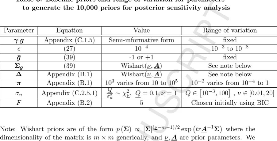
Table 3 indicates the range in 10,000 priors used for posterior sensitivity analysis.
Fig. 10 reports the resulting posteriors for inputs and outputs for Model III. We focus on
changes in the posteriors of inputs and outputs relative to the baseline prior. To minimize
computational costs of this posterior comparison for each of the 10,000 different priors,
we use Sampling-Importance-Resampling (SIR) following Smith and Gelfand (1992) and
Rubin (1987). Given a set of posterior draws{β(s), s= 1, ..., S}for a model with a given baseline prior, say po(β), approximate draws from the same model with an alternative
prior p(β) can be obtained using the SIR algorithm. This attaches weights, Υs = p(β(s))
po(β(s)), to the original draws and resampling is used with these normalized weights avoiding the reuse of MCMC19. All sensitivities are quite small.
Fig. 11 reports the sensitivity of changes in posterior means for structural parameters
of Models I-III to 10,000 different priors. Since the use of SIR does not require new
MCMC computations, it is particularly suited to large-scale prior sensitivity analysis
as in our case. The 10,000 different priors are generated from the baseline prior of
each parameter or block using the hyperparameters of these priors. If the vector of
hyperparameters is collectively denoted by δ∈R∆ new priors are generated usingδ∗ =
δ+κ where κis uniformly distributed in [−B1, B2]∆.
We set B1 = B2 = 10 for hyperparameters that can be defined over the real line
and B1 = 0.001, B2 = 10 for positive hyperparameters. Performing the same sensitivity
analysis experiment when only the priors for the structural parameters are allowed to
change, the changes in posterior means are modest, suggesting that posterior MCMC is
quite robust.
After estimating the shadow PM model, we compute for Model III the posterior
means of relative shadow prices over time for bad outputs from equation (52). As
re-ported in Fig. 12, these prices all decline over time, consistent with historically declining
costs of pollution control. The relative prices of SO2 and NOx are consistent with
esti-mates of control costs from the Integrated Environmental Control Model (Rubin, 2009).
In order to compare the predictive accuracy of the shadow-CM and shadow-PM
models, we compute the marginal posterior of the predictive measures of R. For five
randomly chosen utilities, provided in Fig. 13, R values range from zero to .5. The mean
values range from approximately .01 to about .1, indicating that the shadow-PM model
is strongly preferred to the shadow-CM model.
Finally, in Figs. 14-15 and Table 4 we report for Model III the partial elasticities of
ω in (30) with respect to ωt−1,px,py, π, τ and t. When implementing (32)–(35) we do
not impose monotonicity of profits with respect toω. However, we find that the required
monotonicity is satisfied for 99% of our observations.
Laggedω is the most important variable affecting ω with a positive elasticity of .43.
ReducingpE is the second most important variable with an elasticity of -.41. Reductions
in pK and pL are more important than an increase in the prices of residential and
industrial production. Profits have a very small but positive effect on productivity. All
elasticities except for those of t and τ are significant at the .05 level using a two-tailed
test, indicating little affect of time itself or the aging of capital stock.
5
Conclusions
Using a Bayesian appproach, our contributions to the productivity literature are
fourfold. First, we estimate unique optimal-PM directions for each good input, each
good output, and all regulated bad outputs. Second, we allow the potential endogeneity
of all inputs and outputs. This entails identifying the DDF by assuming a data generating
process for the latent prices as instruments to replace missing prices for the regulated bad
outputs. Then we estimate the DDF jointly with the first-order price equations derived
sulfur, and the uncontrolled pollutant, CO2, are identified using reduced-form equations.
We also estimate the corresponding CM model. Third, we avoid the typical assumption
that firms respond to actual prices by estimating firm-specific shadow prices. Fourth, we
generalize and provide an alternative to the approaches of OP (1996) and LP (2003). We
accomplish this by treating all input and output quantities as potentially endogenous
and deriving productivity as a function of lagged productivity, profits, vintage, time,
and the prices of good inputs and outputs. From this function, we compute TC, EC,
PC, and partial elasticities.
Using MCMC methods, we generate posterior densities for the parameters and latent
variables of our system using an unbalanced panel of 77 U.S. electric utilities for the years
1988-2005. Using Bayesian criteria, the shadow PM model is superior to the shadow CM
model in terms of predictive ability. Optimal directions subject to shadow PM differ
from their typically assumed values (-1 for all bad outputs and all inputs, and +1 for
good outputs). Estimated price distortions for the good inputs indicate that efficient
levels of usage are slightly lower for capital and labor but are moderately higher for
energy. Mean PC is slightly less than .01. The major factors augmenting productivity
are an increase in lagged productivity and a reduction in energy prices. Changes in
posterior means of the structural parameters and the directions are highly insensitive to
a wide range of different priors.
References
Ackerberg, D. A., Caves, K., Frazer, G., 2015, Identification properties of recent pro-duction function estimators Econometrica 83, 2411-51.
Atkinson, S.E., Halvorsen, R., 1976, Interfuel Substitution in Steam-Electric Power Generation. Journal of Political Economy 84, 959-78.
Atkinson, S.E., Halvorsen, R., 1980, A test of relative and absolute price efficiency in regulated utilities, Review of Economics and Statistics 62 (1), 81-88.
Atkinson, S. E., Tsionas, M., 2016, Directional Distance Functions: Optimal Endoge-nous Directions. Journal of Econometrics 190, 301-314.
Borenstein, S., Bushnell, J., 2015, The U.S. electricity industry after 20 years of re-structuring. Annual Review of Economics 7, 437-463.
Caves, D.W., Christensen, L. R., Diewert, W. E., 1982a, The economic theory of index numbers and the mesurement of input, output, and productivity. Econometrica 50, 1393-1414.