Multi objective, multi level, multi stakeholder considerations for airport slot allocation

(1)

1

“Multi-objective, multi-level, multi-stakeholder

considerations for airport slot allocation”

Author:

Fotios Katsigiannis

Supervised by:

Prof. Konstantinos G. Zografos

As a requirement for the module:

MSCI650 - MRes in Management Science Dissertation

Lancaster University Management School

(2)

2

Acknowledgements

I would first like to thank my supervisor Professor Konstantinos G. Zografos. His door

was always open for me whenever I faced challenges with my research. He allowed this

thesis to be my own work but kept me in the right track by providing valuable

comments, ideas and directions.

I would also like to acknowledge Dr. Jamie Fairbrother for granting me access to his

single airport optimisation framework and providing feedback on the algorithmic parts

of my work. Without his input, the quality of this document would not be the same.

I owe a big thanks to my colleague Ramin Raeesi for our endless discussions on various

research topics and ideas, and his insightful comments on the writing of this thesis.

Finally, I must express my profound gratitude to my parents Thanasis and Katerina and

my girlfriend Maria for tolerating my stressful behaviour and encouraging me during

the research and composition of this thesis. Through our talks, my sleepless nights and

anxieties faded away. Thank you.

My studentship and the work reported in this thesis have been supported by UK’s

Engineering and Physical Sciences Research Council (EPSRC) and Lancaster

University Management School through the Programme Grant EP/MO20258/1

“Mathematical models and algorithms for allocating scarce airport resources (OR

MASTER)”.

The author

(3)

3

Abstract

(4)

4

1. Introduction

IATA’s forecast has revealed that air passenger demand will double by 2036 reaching almost 7.8 billion passengers (IATA, 2018a). At the same time, airport capacity remains as one of the main hazards to European air connectivity that will lead to a supply-demand imbalance gap of more than 160 million passengers in 2040 (EUROCONTROL, 2018). In addition, the expansion of existing infrastructure is subject to geospatial, political and financial constraints, which render its implementation rather slow. Therefore, current airport capacity has to be optimally managed to minimise airline and passenger disruption caused by congestion. To do so, IATA has developed a comprehensive policy framework, which provides to congested airports a common tool to distribute airport capacity. This framework is expressed through the worldwide slot guidelines (WSG) as described in IATA (2018b). The current practice is mainly carried out by schedule coordinators, who make use of expert-systems software (e.g. Condor and Score GDC). However, researchers addressing the problem from the economics and the operations research standpoint have highlighted that current practice can be further ameliorated.

The research on airport demand-management mechanisms may be classified into two main categories: (a) pure economic and (b) administrative. (a) mainly focuses on the creation of economic tools (e.g. slot auctions and congestion pricing schemes) while (b) addresses the problem through mathematical programming mechanisms which attempt to model the current regulatory framework and slot priorities. For more information, the reader may refer to the review papers of Gillen et al. (2016) and Zografos et al. (2017b).

Administrative airport slot scheduling has been acknowledged by researchers as an effective airport congestion mitigation technique (Gillen et al., 2016; Zografos et al., 2017b). By taking into account the complex decision process, the literature in the slot allocation has recently adopted a multi-objective decision-making direction, as well as some cunning modelling possibilities. Such modelling considerations allow the inclusion of various rules and priorities when solving for the optimal airport slot schedule. Yet, several policy sections and problem characteristics remain unaddressed.

1.1. Motivation and contributions

The first contribution of this document stems from the analysis of IATA’s WSG, coupled with the critical review of the existing literature (Sections 2 and 3). This step allowed the identification of research gaps that are not currently considered in the literature.

Secondly, the models presented in Section 4 and the solution approach of Section 5 manage to consider some policy rules that have been neglected in previous research attempts. For example, alternative weighted schedule displacement cost functions may incorporate punctuality and year-round operations considerations as specified in IATA’s rules [Section 8.3.6. of IATA (2018b)]. In addition, simple constraint expressions can address section 8.3.5.4. of IATA’s WSG by introducing an upper bound to the maximum displacement occurring for new entrants’ requests.

(6)

6

present a tri-objective administrative mathematical tool, which considers simultaneously three objectives and provides trade-off analysis among them. In brief, the proposed model builds on previous research and formulations so as to propose a tri-objective approach which minimises schedule and maximum displacement while simultaneously considering demand-based fairness as described by Fairbrother and Zografos (2018a). This extends the objective considerations of previous research attempts as none of them has solved for three objectives in parallel.

Concerning the solution approach (Section 5), this paper moves beyond the modelling phase as it proposes a solution approach that is coherent to the current slot guidelines and objectives ensuring schedule acceptability among the different slot priorities. The notion of inter-level tolerance is also introduced since our solution algorithm allows weakly dominated or dominated solutions at the upper slot priorities (e.g. historic) in order to reap better results at the lower levels (new entrants, others). The idea for this approach is based on Stackelberg games and multi-level programming and proves that existing solution approaches (e.g. hierarchical) do not report the most beneficial set of equally efficient schedule alternatives. Given the decision-planning horizon (tactical-strategic), the proposed solution algorithm takes advantage of the value range and the nature of the objectives to provide trade-off solutions, satisfying the operational needs of airlines and some basic IATA policy rules.

Finally, we highlight the potential synergies between MOO and multi-attribute decision making (MADM) techniques by proposing two bi-stage solution approaches which can enhance the current models by allowing the consideration of additional objectives (e.g. CO2 and noise emissions). We highlight our arguments by providing two illustrative examples.

The remainder of the paper is organised in 7 sections. Section 2 presents an overview of the slot allocation process as defined in IATA (2018b). In Section 3, the reader may find a compact, critical literature review that pinpoints modelling gaps in the existing multiple objective slot allocation applications. In addition, Sections 4 and 5 include the proposed models and the description of the prescribed solution approach. Section 6 provides an exploratory data analysis on the case study’s data and discusses the computational results and their potential impact on current practice. In Section 7, we discuss through some simple examples the potential synergies of multi-attribute and multi-objective decision-making techniques in the context of airport slot scheduling. Finally, Section 8 summarises the findings of this work and indicates valuable paths for future work. The document comes with an acronym table (Table 1) explaining some of the most frequent terminology abbreviations used in this paper.

Acronym Explanation

AHP Analytical Hierarchy Process

IATA International Air Travel Association

MADM Multiple Attribute Decision Making

MOO Multiple Objective Optimisation

PSO Public Service Obligations

SCC Schedule Coordination Conference

SSIM Standard Schedules Information Message

[image:6.595.89.510.565.704.2]

WSG World Schedule Guidelines

(7)

7

2. IATA’s slot allocation process

For the past 40 years, the worldwide slot guidelines have been used to alleviate the shortage of global airport capacity in a fair and transparent way. The slot allocation process is the dominant airport demand management mechanism being applied by more than 200 airports of whom more than half are situated in Europe (IATA, 2018c). To further understand the complex decision process, as well as the benefit of our model, this section includes an overview of IATA’s slot allocation process.

In the European Union, each member state is responsible for the airports that lie within their borders. Under this specification, each member state carries out an annual capacity assessment so as to determine whether its airports are subject to capacity shortages. If there is no short-term solution, then the airport may be characterised either as a Level 2 or as a Level 3. Level 2 airports (schedule facilitated)may experience occasional congestion during some operational days, which can be resolved by mutual schedule adjustments by the appointed facilitator and the carriers [Section 4 of IATA (2018b)]. However, in Level 3 airports (schedule coordinated) the situation is more complicated because demand for airport infrastructure is greater than airport capacity in the given period and mutual resolution attempts cannot be made [Section 5.1 of IATA (2018b)]. Once an airport is characterised as “coordinated”, the national aviation authority has to appoint a slot coordinator who should enact independently, neutrally and transparently [Section 5.2 of IATA (2018b)]. The main duties of the coordinator are to [Section 5.5 of IATA (2018b)]:

i) allocate slots to carriers based on the scheduling parameters (e.g. declared capacity) and the slot coordination guidelines and criteria;

ii) communicate to the interested parties the coordination parameters (e.g. coordination time interval), the local guidelines and regulations as well as any additional criteria;

iii) inform each airline about their allocated slots and the list of the remaining slots at the airport;

iv) monitor cancellations on historic1_{slots and the planned versus the actual use of slots} for the application of the use-it-or-lose-it rule2_{[Section 8.6 of IATA (2018b)]; and}

v) identify slot misusing.

It is obvious that the scheduling and coordination parameters are significant for the designation of the initial slot pool as they define the airport capacity and the number of movements that may be scheduled during each coordination interval, hence defining the initial slot pool. Once finalised, the coordinator has to communicate the initial slot pool to the airlines. Respectively, the airlines based on their commercial interests submit their requests for the next scheduling period. The requests are submitted bi-annually before the summer and winter Schedule Coordination Conferences (SCC) [Section 2.2 of IATA (2018b)] using the IATA Standard Schedules Information Manual (SSIM) message format.

Airline requests may fall into two main typologies: series of slots and individual slots. If an airline intends to operate a slot more than five times per scheduling period, then it should submit

a series of slots request. A series request is characterised by the effective period of operation and the time and day of operation. For example, from the 15th_{of July to the 31}st_{of September,} every Tuesday at 14:05. Once all the requests are received by the coordinator, then he is responsible to carry out the initial slot allocation and distribute the slot pool to the airlines

1_{The Historics baseline date as well as the use-it-or lose-it-rule determine historic precedence. Ad hoc} operations are not eligible for historic precedence [Section 8.7 of IATA (2018b)].

(8)

8

according to the slot allocation principles described in sections 8 and 9 of IATA (2018b). At this stage, the only slot typology that is considered is slot-series (Zografos et al., 2012). On the contrary, individual slots may be requested up to a few days before the actual day of the operations subject to the approval of the coordinator.

Following the initial slot allocation, during the SCC the interested stakeholders (e.g. coordinators, airport and airline representatives, coordination committee etc.) meet and discuss beneficial adjustments to the draft schedule prepared by each coordinator. Such adjustments mainly serve the resolution of timing conflicts of connecting flights. In the post conference activity, the carriers should decide whether it is appropriate to operate each slot and may retain, return or modify it. In case new or modified requests cannot be accommodated, then the coordinator should offer the available slot that is closer to the requested [Section 9.13 of IATA (2018b)].

The models presented in the following sections, concern the initial slot allocation, which largely defines the effectiveness of the SCC and the overall effectiveness of the airport schedule. The guidelines and the criteria of the initial slot allocation process are discussed and presented in the following section.

2.1. The initial slot allocation criteria and guidelines

The rules included in this section can be mainly found in section 8 of IATA (2018b). The principles, priorities and criteria described, aim to serve the interests of the travelling public, the airlines and the other participating actors. In addition, they ensure a fair and transparent treatment of all airlines boosting competition and ensuring airport connectivity (IATA, 2018c). Principles and general priorities

The coordinators should firstly take into account the slot allocation principles [Section 8.1.1 of IATA (2018b)], which provide definitions of historic precedence, series of slots etc. In continuation, the general priorities apply [Section 8.2 of IATA (2018b)]. At this point, the series of slots have a higher priority than ad hoc services and other operations. This part of the document is inherently incorporated to the initial slot allocation process, as it is only the series of slots that are considered in this stage.

Primary criteria

(9)

9 Additional criteria

Following the initial criteria, the additional rules ensure other operational objectives such as flight connectivity between airports, competition as well as the requirements of the travelling public and the local community [Sections 8.4.1.a-e of IATA (2018b)]. In brief, slots with a larger effective period of operation should have priority (8.4.1.a.) while the type of service and market should be prioritised based on the interests of the airport and the local community (8.4.1.b.). In addition, coordinators should take into account competitive factors (when rejecting slot requests) and curfews at other airports (8.4.1.c.d.). Finally, the requirements of the shippers and passengers must be met as far as possible (8.4.1.e.).

Displacement criteria

Given that all the additional criteria are considered, and the time requested by the airline is not available, the coordinators should displace the airline’s slots based on the principles described in sections 9.9.3.a-f of IATA (2018b). According to this part of the document, new offers should not be made placing the carrier in a less favourable position than the one currently held. Therefore, offers should be made either within the requested and the historic time (9.9.3.a.), or within the specified flexibility limits (9.9.3.b.). However, the disclosure of flexibility preference data should not place carriers in a disadvantageous position (9.9.3.d.). Carriers may also communicate their willingness to accept counter offers if the requested time is not available (9.9.3.c.). The last two parts of this section dictate that frequent services should not get different service times unless allowed by the airlines (9.9.3.e) and that for paired requests (having an arrival and departure time requested) the turnaround time has to be respected avoiding additional ground times (9.9.3.f).

Punctuality and performance

Even though historic slot rights are granted based on the use-it-or-lose-it rule (usage above 80%), the performance and usage of all slot types is assessed by the Slot Performance Committee and it is monitored at the SCCs bi-annually. As specified in section 8.9 of IATA’s WSG, intentional slot misuse may result in lower priority for future slot requests for each carrier, while sanctions may also apply. In any case, the allocation of the slots happens after the consultation of the Coordination Committee or the Slot Performance Committee, which determine for each series of slots the percentage of slots that were operated in a benevolent way.

Local guidelines - Public service obligations (PSO)

(10)

10

the work of Bråthen and Eriksen (2018). Obviously, similar regulatory frameworks may exist in other areas of the world3_.

Decision horizon

A point which is currently overlooked, is the decision horizon in which the slots are allocated. Currently, it is believed to be six months. Conversely, by closely examining the deadlines disclosed in the first pages of IATA (2018b), we understand that the time that the coordinator has to allocate the slots is far less than that. Namely, in IATA (2018b) it is mentioned that airlines must submit their requests 33 days before the SCC (19th_-21st_{of June 2018). Once} airlines have submitted their requests (e.g. no later than 17th_{of May), the coordinators have to} carry out the initial slot coordination up to 12 days before the SCC (e.g. no later than 7th_{of June} 2018). That means that the coordinators have 22 days at their disposal to draft the initial slot schedule. Therefore, the decision timeframe is of tactical rather than strategic nature. Henceforth, this factor may act as a constraint to the timeframe of the solution approaches considering IATA’s WSG.

Having provided an analytical overview to the regulatory framework of the initial slot allocation process, we may now present an explanation of the SSIM format and action codes in which slots are submitted during initial slot submission deadline (-33 days from the SCC).

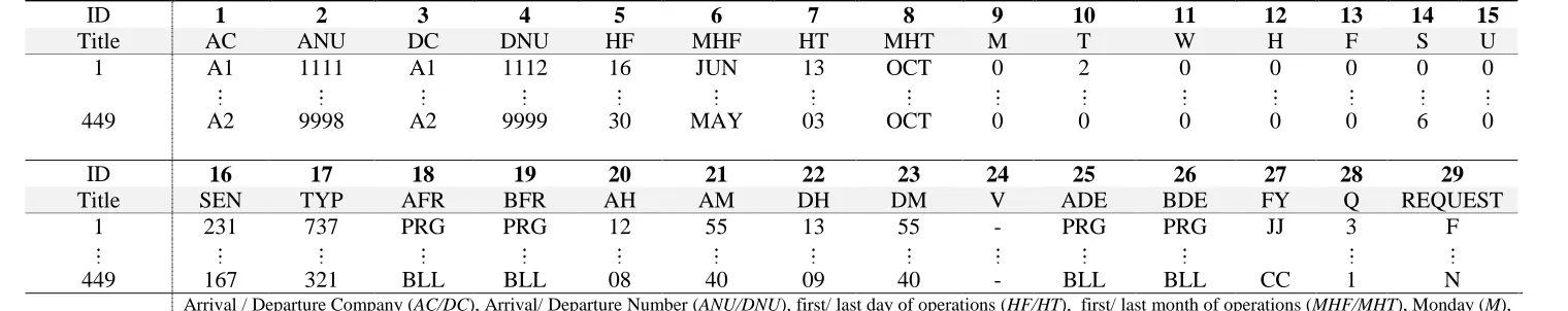
2.2. The SSIM slot request format

The most crucial input in the initial slot allocation process is the slot requests themselves. To better understand the factors that are taken into account during the decision process, there is need to provide the information that the coordinator has in his disposal when drafting the slot schedule. To do so, we will provide a compact guide on the standard SSIM format in which requests are submitted.

Under the SSIM protocol, each airline sends a message to the slot coordinator with all the requests that it wants to submit to the current airport. The message is composed by three main parts: the message header, the message body (flight detailed request) and the footnotes. The header contains four pieces of information in the following format:

 The first three characters are the type of request (e.g. SCR: slot clearance request/reply);

 Another three characters represent the scheduling season indicator (e.g. S19: Summer 2019);

 The following five characters are the day that the message was sent (12AUG :12/08); and

 The last three characters define the airport to which the airline sends the message (e.g. LHR: London Heathrow)

Consequently, an example SSIM header would be: SCR S19 12AUG LHR.

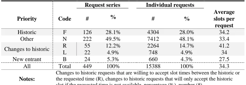
The second component of the SSIM is the flight detail lines which is the main body of the request. Each line represents a slot request and may have multiple pieces of information. Requests can be submitted as arrivals, departures or as paired requests having both an arrival and a departure slot. Once all airlines send their requests to the airport, the coordinator extracts the flight detail lines and creates a table with all the slot requests submitted to the airport. In addition, in the ‘REQUEST’ column the coordinator includes action codes characterising the

(11)

11

priority type of each request (column 29). An example of such a table as well as an explanation of each column is given in Table 2. Likewise, the dataset that was used for our computational study (Section 6) is of similar form to Table 2.

The action codes (column 29 of Table 2) used by the coordinator to classify the requests may take the following values:

• A: acceptance of an offer – no further improvement desired; • B: new entrant request;

• F: historic request;

• L: change to historic which will accept only the requested or the historic slot; • N: new request which is not entitled of new entrant status;

• R: change to historic request which will accept any slot between the requested and the historic slot times;

• I: change to historic slot extending to a year-round operation; • Y: new slot request willing to operate as a year-round operation; and • V: new entrant request extending a year-round operation.

(12)

12

ID 1 2 3 4 5 6 7 8 9 10 11 12 13 14 15

Title AC ANU DC DNU HF MHF HT MHT M T W H F S U

1 A1 1111 A1 1112 16 JUN 13 OCT 0 2 0 0 0 0 0

449 A2 9998 A2 9999 30 MAY 03 OCT 0 0 0 0 0 6 0

ID 16 17 18 19 20 21 22 23 24 25 26 27 28 29

Title SEN TYP AFR BFR AH AM DH DM V ADE BDE FY Q REQUEST

1 231 737 PRG PRG 12 55 13 55 - PRG PRG JJ 3 F

N

449 167 321 BLL BLL 08 40 09 40 - BLL BLL CC 1

Notes:

[image:12.842.46.806.172.323.2]

Arrival / Departure Company (AC/DC), Arrival/ Departure Number (ANU/DNU), first/ last day of operations (HF/HT), first/ last month of operations (MHF/MHT), Monday (M), Tuesday (T), Wednesday (W), Thursday(H), Friday (F), Saturday (S), Sunday (U), Seats Expected (SEN), type of aircraft (TYP), airport of origin (AFR), last stopover airport (BFR), Arrival/Departure Hour (AH/DH), Arrival/ Departure Minute (AM/DM), Overnight indicator (can be 1 or 2 if the aircraft will depart after one or two days and ‘-‘ if it departs the same day) (V), next stopover airport (ADE), destination airport (BDE), Service codes for the arrival and departure flights (FY where J/F: schedule passenger/ cargo flight, C/H: chartered passenger/cargo flight, P: positional, X: technical, D: general or private, N: Business aviation/ air taxi), frequency indicator (Q), request priority action code (R).

(13)

13

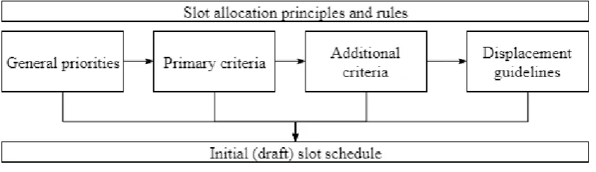
2.3. Summary

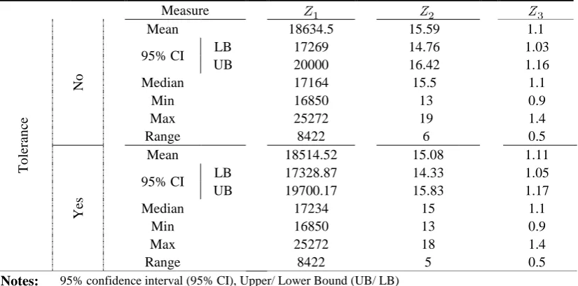
The aforementioned guidelines compose a structured sequence of criteria and priorities that is depictured in Figures 1 and 2. Figure 1 groups the criteria at a higher level while Figure 2

presents a more detailed picture. In detail, Figure 2 is a schematic representation of the rules and priorities ordered hierarchically based on the verbal expressions given in the updated version of IATA’s WSG.

From both graphs, we understand that the complexity of the focal decision context as well as the inherent hierarchies that lie within the framework itself demand the consideration of all the rules and priorities when attempting to prescribe a mathematical model aiding in the current slot allocation process.

[image:13.595.90.509.129.250.2]

Moreover, even though PSO route priority is not explicitly included in IATA’s WSG, it has to be considered because local or regional guidelines prevail IATA’s rules. Therefore, such routes constitute an additional priority which is hierarchically superior to historic slots and has to be allocated before them [Article 9 of the Council Regulation No 95/93 (1993)].

Figure 1: Overview of the initial slot allocation rules

[image:13.595.104.501.325.536.2]

(14)

14

3. Previous related work

This section includes a critical discussion on the multi-objective slot scheduling models that consider the IATA’s regulatory framework (Figure 2). As mentioned before, the majority of the most congested airports follow IATA’s world schedule guidelines (WSG) to manage airline demand for their resources. In contrast, the airports lying within the U.S [except for John F. Kennedy International Airport (JFK), LaGuardia Airport (LGA), and Ronald Reagan Washington National Airport (DCA)] do not follow this set of rules. In this work, we will only examine multi-objective models, which consider airport operations under IATA’s WSG. Administrative slot scheduling was firstly addressed via integer programming in Zografos et al. (2012). Since then, researchers have contributed to this stream of research by considering multiple objectives and modelling additional rules and specificities of the regulations. The existing MOO models may be divided based on the decision context that they consider. The majority of MOO formulations consider IATA’s WSG while a few of them address the U.S decision-making context (Jacquillat and Odoni, 2015; Jacquillat and Vaze, 2018; Pyrgiotis and Odoni, 2015). IATA based models attempt to solve the slot allocation problem for the whole scheduling period while considering series of slot requests and as many of IATA’s WSG as the can. Nevertheless, the US-based models consider individual slot requests and only solve for a single day of airport operations. At this point, it is worth mentioning that the former model typology has attracted greater research effort because of the modelling difficulties (slot priorities, series of slots etc.) and its widespread usage by the majority of the most congested airports. A more general review of the total corpus of the MOO slot scheduling models was presented by Katsigiannis (2018a).

The models presented and discussed in this work, take into account IATA’s WSG decision context. Through the cross-tabulation of the relevant literature (Table 3), we understand that models with such policy considerations are rather recent and limited (Fairbrother and Zografos, 2018a, 2018b; Ribeiro et al., 2018; Zografos and Jiang, 2016; Zografos et al., 2017a). By examining Table 3, we conclude that there are still exist some sections of the policy framework that have not been addressed either because of the modelling and computational hazards or because of the lack of information, data and systematic consideration of the policy framework. To provide a brief discussion on the relevant models, we will analyse the existing literature on a chronological order. Firstly, the paper of Zografos and Jiang (2016) proposed two bi-objective models which minimise two different schedule displacement metrics along with a fairness index. In detail, they introduce a measure of fairness, which is expressed via the proportion of displacement that each airline experiences in relation to the number of requests that it submits. If the fairness index is different from one, then the airline experiences disproportional schedule delay (higher or lower) to the number of requests that it makes. In the second formulation that they provide, they introduced a weighted displacement metric capturing the size of the operating aircraft and the flight distance (short haul, long haul). The incorporation of such weights allows the model to address the needs of the travelling public as flights with longer distance and more passengers receive a relative priority on the schedule displacement objective.

(15)

15

slot priority, i.e. considering historic, new entrant and other requests sequentially. To do so, they update the slot pool once all the slots in each priority level are allocated. Their solution approach generates the set of efficient solutions at each level and proceed to the lower levels based on that setting.

By attempting to address more of the IATA’s rules and priorities, Ribeiro et al. (2018) provided a more realistic formulation considering additional criteria. In brief, they explicitly considered the “changes to historic slots” as a different priority, providing a more accurate definition of

the slot-pool and the following slot types (new entrant and other requests). In addition, they modelled the displacement criteria described in section 9.9.3 of IATA’s WSG. As for the considered objectives, they formulated the problem as a quart-objective weighted cost function minimising the number of rejected slots, the maximum and schedule displacement objectives and the number of violated slot assignments. The weights of the objective function mimic the lexicographic optimisation method, thus prioritising the objectives. Their model was tested on data obtained from two medium-sized Portuguese airports. However, the case study did not allow the consideration of the rejected slots objective as the requests and the capacity did not result in slot rejections.

Regarding the solution approach, the paper of Ribeiro et al. (2018) employs a different method than previous research. Instead of restricting the remaining capacity, they solve the problem for each priority level lexicographically. This approach is better suited to the nature of the problem as it captures to a certain extent the multi-level, hierarchical interdependencies existing between the different types of slots. Albeit, a major drawback of their approach is that the objective function is not suitable for the commensurable nature of the criteria. This argument stems from two major points. Firstly, the criteria are not expressed with the same measurement scales (e.g. maximum and total displacement) and the weights are not normalised (they are all significantly greater than one). Secondly, the lexicographic-like approach explicitly considers the preferences of the decision maker(s) when providing the weights for the objectives. At the same time, it does not provide a systematic way of exploring the total set of efficient solutions. Finally, during the analysis of their results, the authors only provide bi-objective trade-off analyses rather than a quart or tri-objective approach.

As we have schematically demonstrated in Figure 2, fairness, transparency and non-discriminatory considerations are omnipresent in the slot allocation decision process. In this context, Fairbrother and Zografos (2018a) built on the work of Zografos and Jiang (2016) and introduced a demand based fairness index which considers the peak requests of each of the airlines. Therefore, this index is equal to one when an airline receives proportional delays to the peak requests that it makes. The authors moved beyond the proposal of this objective and constructed a budget mechanism that allows airlines to distribute the total displacement of their flights based on their own preferences. This attempt is one step closer to the operational needs of airlines but is limited by the absence of preference data.

(16)

16

increased number of decision variables and constraints. Second are the flexibility range parameters which are applied uniformly to all requests. This is something that contradicts the specifications of the IATA guidelines as each airline should provide its own flexibility range for each of their slots. Finally, it is not clear how schedule displacement is calculated since flexibility acts like an allowable slack which is not counted in displacement cost functions. In any case the disclosure of flexibility information should not put airlines in an unfavourable market condition. Hence, differentiated flexibility bounds for each airline and linear functions of disutility could account for this policy requirement.

At this point it is worth mentioning that there is another stream of research which addresses airport slot scheduling at the airport-network level, hence capturing slot complementarities among inter-connected airports. In this stream of research, two multi-objective approaches exist (Corolli et al., 2014; Pellegrini et al., 2017). The model of Corolli et al. (2014) minimises the schedule displacement as well as the expected queuing delays, while the model of Pellegrini et al. (2017) has cost functions minimising the costs of violated slots and the displacement of coupled or independent slots accordingly. Even though this stream of research is of great interest, the models above are not tabulated in Table 3 since the scope of this work focuses on the single airport level.

To summarise, the existing attempts capture many modelling aspects of the focal problem. Albeit, there still exist research gaps and opportunities, which can be addressed that fall into four main categories:

i) Modelling of the unaddressed regulations and priorities;

ii) Suggesting additional or alternative cost functions and constraints that are more accurate, efficient or model additional aspects of the problem;

iii) Simultaneous optimisation of more objectives; and

iv) Devising solution approaches that can capture the interdependencies between the different decision levels (slot hierarchies).

(17)

17

Primary criteria Duration Additional criteria Displacement criteria Fairness Flexibility PSO routes

Model 8.3.2 8.3.3 8.3.4,

8.3.5 8.3.6 8.4.1.a 8.4.1.b. 8.4.1.c.

8.4.1.d,

9.7.3.d 8.4.1.e 9.9.3.a 9.9.3.b 9.9.3.c 9.9.3.d 9.9.3.e 9.9.3.f

5.5.1.a, 8.1.1.j

8.3.6.1-2, 9.7.3.b

CR 95/93 (1993) Zografos

and Jiang (2016)

     * _ _ _ _ _ _ _ _* _ _ _ _

Zografos et al. (2017)

             * _ _ _ _

Ribeiro et

al. (2018)           

* _ _ _* _ _ _ _

Fairbrother and Zografos

(2018a)

             * _ _ _ _

Fairbrother and Zografos

(2018b)

          * _ _* _ _ _ _* _

Addressed _ _ _ _ _ * _ _ _ _ _ _ _* _ _ _ _* _

Notes:

Historic slot requests (8.3.2.), Changes to historic slots (8.3.3.), New entrants rules (8.3.4., 8.3.5.), Year round operations (8.3.6.), Effective period of operation (8.4.1.a.), Type of service and market (8.4.1.b.), Competitive factors when rejecting slots (8.4.1.c.), Curfews (8.4.1.d., 9.7.3.d.), Requirements of shippers and travellers (8.4.1.e.), offers shall not place airlines in less favourable conditions than the ones held (9.9.3.a.), acceptable/ unacceptable offers (9.9.3.c.), consistent turnaround times (9.9.3.f.), flexibility sections (9.9.3.b., 9.9.3.d. 9.9.3.e.), addressed/ accurately addressed (/), not addressed (), * partially considered, Fairness stands for transparency and non-discrimination of airlines.

(18)

18

4. Slot allocation models with multiple objectives and multi-level considerations.

In this section, we present a tri-objective slot allocation model that considers efficiency (schedule and maximum displacement) and fairness objectives. Our model builds on previous research by incorporating the modelling capabilities of various models already existing in the literature. For instance, the base problem is adapted from the formulation of Zografos et al. (2012), while the fairness cost function that we consider has already been defined in the literature by Fairbrother and Zografos (2018a). Yet the following formulation is the first to model all the objectives simultaneously, thus being able to provide trade-off analysis among them. Moreover, in 4.2 we propose and prove that the tri-objective slot allocation problem (TOSAM) can be modelled as a multi-level problem. The originality of this approach stems from the fact that no other research considers the slot allocation problem in a multi-level manner. This consideration extends and formalises current modelling and solution approaches and may potentially sparkle new research trends and interests.

4.1. A Tri-Objective Slot Allocation Model (TOSAM)

Models addressing the IATA’s WSG decision context have to account for series-of-slots requests as per Section 2. Moreover, the decision-planning horizon is set to be the whole scheduling period, rather than a single day. The backbone of the presented model is a modified version of the work of Zografos et al. (2012), however some modifications are made serving computational efficiency and the incorporation of the multi-objective considerations. In the following subsections we present the notation required (input data sets, parameters, decision variables) so as to better understand the main body of the model (equations 4.1.- 4.8.).

4.1.1. Formulation

Input data sets

set of airlines denoted by ;

set of request series denoted by ;

set of request series of airline ;

, set of arrival (departure) series; set of paired requests indexed by ; set of days in scheduling season denoted by ;

set of days that slot m is to operate;

set of capacity time scales indexed by ;

set of time intervals per day based on scale indexed by , s;and set of movement types denoted by .

Input parameters

- requested time for slot series ;

- , as peak times

Fairbrother and Zografos (2018) define periods of duration where airline demand exceeds airport capacity;

(19)

19

- capacity for movement for period on day based on time scale ;

- ; and

- , the proportion4_{of peak requests}

of airline . Decision variables

-

Base Constraints

Constraints (4.1) ensure that each of the slots will be allocated to a time. Moreover, constraints (4.2) are rolling capacity constraints for each type of movement i.e. arrival, departures, or total movements. The last type of constraints (4.3) are turnaround time constraints which define that the time difference between two paired requests should not be less than the initially requested difference between them (minimum turnaround time) and larger than a specified limit. In the absence of preferences regarding the maximum turnaround time, its value can be set equal to an operationally viable value or infinity.

Please note that the precedence constraints defined in Zografos et al. (2017, 2012) are not required as the programmatic parsing of the input data renders them redundant.

Cost functions

Where:

,and;

Expression (4.4) states that all objectives are minimised. Equations (4.5) and (4.6) define the schedule and maximum displacement cost functions. Equation (4.7) defines the third objective

4_{Fairbrother and Zografos (2018) refer to this index as contribution of airline to congestion.}

(4.1) (4.2) (4.3)

(4.4)

(20)

20

of the proposed model expressing the maximum deviation of the fairness index ( from 1. When the fairness index is equal to one, then the proportion of displacement allocated to airline is completely analogous to its contribution to congestion. If equation (4.8) is less than one, then airline is experiencing less displacement in relation to the peak requests that it has submitted. Obviously, for values of above one, the displacement that the airline will experience is greater than the proportion of its requests at peak times. Therefore, objective function is minimised as we would like expression (4.8) to take values close to zero. ε-type constraints

Scalar approaches may result in reduced computational times, but they cannot generate satisfactory portions of the efficient solutions’ set. In addition, commensurable objectives which are not expressed in the same units should receive either normalised or justifiable weights (Takama and Loucks, 1981). Therefore, there is need to modify the base problem described in above to incorporate those two problem characteristics.

The state of the art in tri-objective solution algorithms employ expanded, generalised variants of the ε-constraint method (Haimes, 1971). Especially, they constrain the objective values of two of the three cost functions by using a list of upper bounds while optimising the third objective (Boland et al., 2017). In order to employ such solution algorithms two of the objectives have to be expressed in the form of linear constraints. By taking advantage of the scales of the objectives, we chose to re-model cost functions and . That is because the width of their efficient solution values is smaller than that of the total displacement. For example, fairness stops being a binding objective for values above 1.5 (where the carriers receive 2.5 times less or more displacement than their peak requests), while maximum displacement cannot exceed the total duration of the number of time intervals within a day. On the contrary, the range of is by far greater even by the product of the widths of the other two objectives.

Given all the above, objectives and can be written linearly with the use of expressions (4.9 – 4.12).

Constraints (4.9 - 4.10)5_{ease the definition of the maximum displacement objective (} _{) by} limiting it under while constraints (4.11- 4.12) help bound the fairness objective ( ) under

.

5_{It is easier for pre-solving to compute tighter bounds on the variables that are in the constraints. With} the formulations that currently exist in the literature, solvers may struggle to find solutions.

(4.9) (4.5) (4.10) (4.5)

(21)

21

Having provided the formulation of our base model, we may now suggest some additional modelling considerations that capture some of IATA’s WSG requirements, which have not yet been addressed.

4.1.2. Alternative weighted schedule displacement functions

In this subsection, we introduce two novel weighted models that manage to model performance and punctuality [Sections 8.4.1.b and 8.9. of IATA (2018b)] and prioritise year-round operations [Section 8.3.6. of IATA (2018b)].

4.1.2.1. Introducing punctuality and performance considerations

Performance and slot misuse have yet to be addressed in the literature. As described in Section 2.1, airlines’ ill slot performance and slot misuse may result in sanctions and lower slot priorities. Slot monitoring is conducted in a long-term manner in order to give to airlines the opportunity to correct their performance regarding each slot in following seasons. The irregularities that the committees responsible detect, mainly fall into the following three categories (COHOR, 2018):

 Flights that are operated without allocated slots;

 Flights operated in different conditions than those specified in the allocated slot; and  Unused slots which deprive the airport of valuable capacity resources.

To consider the latter two, we may take advantage of the slot utilisation ratio ( ) provided by the Slot Performance Committee that monitors and determines slot usage before the SCCs. At the same time the punctual flight operations serve the interest of the travelling public and the shippers [Section 8.4.1.b of IATA (2018b)].

Therefore, given that there are historic records of airline requests, let:

- be the set of scheduling seasons up to the current scheduling season that airline holds slot , starting from season and it is indexed by ; - : be the utilisation ratio of slot at scheduling season ;

- ; and

- be the set of requests at period j and the set of requests by airline a submitted at period .

Then the performance index of each airline at the current scheduling period is:

Then and the relative performance index for airline may be calculated as follows:

The practical meaning of equation (4.13) is that for all the slots that airline is currently holding, we calculate the historical performance and we divide it by the number of periods that the airline operated the slot . As for equation (4.14), we divide the (4.13) (4.5)

(22)

22

historical performance of the airline by the average performance of all airlines operating in the airport. Therefore may take values based on the following expression:

Due to the fact that equation (4.14) is a relative measure, it takes into account the overall historical slot usage in the current airport, accounting for disruptions occurring to all airlines operating in the airport. Hence, it penalises airlines that faced internal disruptions that were mainly caused by ill managerial or operational planning (e.g. poor maintenance). In addition, the index may capture inter-seasonal slot misuse and penalise airlines that constantly underperform. Please note that the provided formulation may even account for shared operations as can be equal to one for more than one values of .

Given those updated modelling considerations, the objective function for total displacement is modified as per (4.16):

This formulation attempts to facility an airline efficiency-based airport resource allocation that takes into account historic slot usage.

4.1.2.2. Introducing year-round and effective period priority considerations

Another modelling gap stems from the absence of prioritisation for year-round requests and services that have larger effective periods. Section 8.3.6. of IATA (2018b) states that year-round requests of all priority types should get priority over other requests of the same priority. Moreover, requests covering longer periods of operations should receive larger priority [Section 8.4.1.a. of IATA (2018b)].

To capture those two specifications, we have to introduce the service continuity index denoted by the Greek letter σ (sigma), described in expression (4.17) along with some extra input sets and parameters.

Let:

- be the set of days that slot is to operate in the scheduling season having days and being the effective period that the slot will operate. - is the number of weeks in the scheduling season; and

- .

Then the service continuity index for slot is:

To explain (4.17) in non-technical terms, if the request is due for a year-round operation then it receives two times the weight that a single period request of the same duration would receive. The right part of the index is the effective period index. This sub-index is a fraction consisting of the number of weeks that a slot is requested for divided by the number of weeks of the scheduling period .

(4.15) (4.5)

(4.16) (4.5)

(23)

23

An updated version of the schedule displacement objective accounting for service continuity would be:

4.2. A multi-level optimisation framework in tri-objective slot allocation modelling

Multilevel decision-making is inspired by game theory and especially by the Stackelberg leadership model (Stackelberg, 2011). Multi-level programming techniques are used in order to address the compromises that are needed to be made between the interactive decision entities which compose a hierarchical organisation or decision process (Lu et al., 2016). The compromises and the tolerance of the upper decision entities increase the welfare output of the system since the aggregate benefit of the individual cost functions is larger than optimising the upper decision levels without foreseeing the benefit of the lower decision entities (Tesoriere, 2017).

To provide some insights and definitions from multi-level decision-making, we will refer to the decision entities of the upper and lower levels as leaders and followers. The decisions of the different entities are applied sequentially with each of them optimising their respective cost functions independently. The architecture of this decision process implies that the leader has priority when determining his own decision, while the followers react and constrain their decision having perfect information (full knowledge) of the decisions of the leaders. Even though leaders’ movements and decisions greatly affect followers’ decision space, the decisions of the followers’ do not explicitly affect the feasible decision space of the leaders. The hierarchical decision structure described above, appears in various real-world management problems. A potential application of multi-level programming would be to model the airport slot allocation with IATA’s hierarchies as a multi-level problem.

CLAIM 1.

The airport slot allocation decision-making process defined by IATA’s slot priorities is a multi-level problem and can be modelled as one.

Proof.

By accepting that Claim 1 holds, we may continue by providing a multi-level formulation of the focal problem. We already mentioned that the requests submitted for each slot-scheduling season might fall into four main priority types: historic, changes to historic, new entrant and other requests. Therefore, the set of the requests is a union of all the requests belonging to those priorities. Following the notation in section 4.1 let:

- be the set of priorities denoted by where and

stand for historic, changes to historic, new entrant and other series of requests respectively. Then, the whole set of requests can be expressed as: ;

(1) The decision process is composed by interacting decision making units with a hierarchical structure, i.e. slot priorities;

(2) The decisions executed by the following levels are defined after and only after the decisions of the leading levels;

(3) For each level, the objectives are optimised independently without considering following levels’ actions, yet following levels are constrained by the decisions of the leaders; and

(4) The influence of the decisions of the leading levels is reflected in the feasible and decision spaces of the lower levels.

(24)

24

- is the set of levels, which are leaders to including . - is the set of levels, which are followers to including . - be a vector of decision variables defined at level , where is the cardinality of the set of requests of priority and the feasible space of the variables;

- be

the vector of the cost functions of level ;

-The expression of the vector-valued cost functions’ criterion space for all four levels

is with being

the feasible criterion space ;

- is the set of constraints of level

- are the constraint conditions of the

four levels with being the number of constraints for all four levels; and

- be the restricted feasible design space of the decision variables of level based on additional constraints on the decision variables, such as upper and lower bounds on the ε-type constraints of Section 4.1.

Given the above notations, we may now provide a general definition of the ML-TOSAM. DEFINITION 1.

For

the ML-TOSAM is defined as follows:

(historic level)

Subject to:

Where for each given by the historic level, solve the problems of the second, third and fourth following priorities.

(changes to historic level)

Subject to:

Where for each , given by the historic and changes to historic level, solve the problems of the third and fourth following levels.

(new entrant level)

Subject to:

Where for each , , given by the historic, changes to historic and the new entrants level, solve the problems of the third and fourth following levels.

(other level)

Subject to:

(4.19.a) (4.5) _(4.19.b) (4.5)

(4.19.c) (4.5) (4.19.d) (4.5)

(4.19.e) (4.5) (4.19.f) (4.5)

(25)

25

Please note that the hierarchical structure in Definition 1 is typical of nested multi-level programming. ML-TOSAM can be also written in a condensed, recursive algorithmic manner (Algorithm 1).

Algorithm 1:The recursive ML-TOSAM

The generic definition of the ML-TOSAM allows us to define the solution concepts

that occur from its recursive formulation in Algorithm 1. The definitions and solution

concepts are an attempt to extend a similar tri-level single-objective formulation

proposed by Lu et al. (2012).

DEFINITION 2.

The solution concepts of the ML-TOSAM are defined as per (i)-(x).

(i) The constraint region of the quart-level problem is:

(ii) The feasible decision space of level which has followers and leaders is generally defined:

(iii) The feasible decision space of the changes to historic level (second) for each set of decision variables given by the historic level is:

(iv) The feasible set of decision variables of the new entrant level (third) for each set of decision variables given by the historic and changes to historic levels is:

(v) The feasible set of the other level (fourth) for each set of decision variables given by the historic, changes to historic levels and new entrant levels is:

input:

output: list of multi-level trade-offs

Define:recursive ML-TOSAM ( )

; # List of solutions is initialised as empty

if Γ then

Stop; # termination of Algorithm 1

else:

for each repeat:

; ;

recursive ML-TOSAM ; # move to the next level

return ;

recursive ML-TOSAM ( );

(26)

26

(vi) The rational reaction of the other (fourth) level:

Which practically means that the only reaction that others may have is the minimisation of the values of their objectives based on the feasible decisions of the leading levels.

(vii) The rational reaction of the new entrants (third) level is:

Equivalently, the reaction of the model at the new entrants level is to minimise its own objective function based on the leading levels’ (historic, changes to historic) decision variables and the rational reaction set of the lower levels (other).

(viii) The rational reaction of the changes to historic (second) level is defined accordingly:

Where the reaction of the model at the changes to historic level is to minimise its own objective function subject to its feasible space, based on the leading level’s (historic) decision variables and the rational reaction set of the lower levels (other, new entrants).

(ix) The inducible region (Chang and Luh, 1982) of the quart-level problem is:

The leader can only assume (induce) the followers’ behaviour since he has limited (implicit) information. The inducible region of the ML-TOSAM is the values (inducible values) that belong to the rational reaction set of the changes to historic level and result to feasible decision variable values for all following levels (feasible for the bottom level). The definition of the inducible region is essential in order to yield the necessary and sufficient conditions for the optimal solution.

(x) The efficient trade-off set for the quart-level problem is:

(27)

27 4.2.1. Discussion

The multi-level formulation provided in (4.2) indicates that in order to find the most beneficial schedules, there is need to consider all the feasible combinations of the decision variables that yield minimum values for the objectives of each level. Moreover, we chose to address explicitly the historic slot priority to provide a robust modelling framework. We mention that because in cases where the capacity of the airport is inferior to the capacity during the previous scheduling season, it will be meaningful to solve for this priority level as well. Obviously, in the general case where the capacity remains the same, the historic slots will be allocated having zero displacement. In any case, our modelling framework allows the consideration of both options. Multilevel optimisation models are not malleable by standard mixed integer programming techniques and software. Moreover, there are no universal efficient algorithms that can aid in their solution (Cappanera and Scaparra, 2010). The exploration of all feasible points even for the single objective problem is a rather demanding task in terms of computational demands having a complexity of . In the literature, quart-level, multi-objective models are treated via fuzzy, heuristic or goal programming solution approaches (Sakawa and Nishizaki, 2012), which can be also applied for the solution of the ML-TOSAM. However, in the future, with the technological progression and the upgrades of standard computational machines, it would be interesting to see exact methods implementing and solving the ML-TOSAM.

In the next section, we present a recursive search algorithm along with some hybrid quasi-exact solution approaches which constrain the feasible space of each decision level, thus resulting in reduced computational times and complexity abiding by the decision horizon’s requirements. The proposed solution approaches exploit the slot hierarchies in order to reduce the number of follower’s strategies to be evaluated.

5. Solution approach

Multi-level approaches explore greater proportions of the feasible decision space but come with increased computational complexity. This issue can be resolved by restricting the feasible space of each level with sensible constraints according to the operational requirements of the real-world problem (e.g. upper bound to the maximum displacement objective, or a threshold to fairness). Yet, one issue renders the solution generation more difficult; in multi-level approaches the generation of Pareto optimal solutions is more complex.

To tackle this issue, in the following sections we will try to respond to the following questions: How to produce efficient solutions that capture the compromises of the leading decision entities? Can we produce multi-level, multi-objective efficient solutions? How can we reduce the feasible space of the decision levels without losing meaningful solutions?

5.1. Preface and definitions

(28)

28 DEFINITION 3.

The TOSAM of decision level is , where is restricted by a set of constraints and is a vector of three linear functions such that

with being the feasible set in the criterion space. Please observe that the objective functions are now defined only based on the decision variables of the current level. That is because in the solution approaches that we will present (except for Algorithm 2), we allocate only the slots of the current decision level, who are considered fixed in the following decision levels. That is a hybrid approach between the hierarchical solution algorithm of Zografos et al. (2012) and the multi-level formulation of Section (4.2). To apply a genuine multi-level solution approach, for each level we should allocate all slots, yet calculating the objective values only for the slots belonging to the current priority level. Based on this setting, by adjusting the notion of Pareto (non-dominated) efficiency to our problem typology we get:

DEFINITION 4.

We will refer to solutions as weakly efficient, if there is no other such that . Given that is weakly efficient, then is a level-based weakly nondominated point.

DEFINITION 5.

For solutions that there is no other point such that

, we will refer to them as level-based Pareto optimal (or efficient or non-dominated). Obviously if is Pareto optimal then is a nondominated

point.

PROPOSITION 1.

For a level , if , and is nondominated point then all the aggregate solutions given by lower levels based on this point, are nondominated points based on level .

Proof. Follows immediately by Definitions 4 and 5. DEFINITION 6.

For each rolling solution of levels, that is a nondominated solution based on level , then the schedule-wide solution is nondominated based on level .

PROPOSITION 2.

For a level , if all the solutions given by , are dominated points then all schedule-wide solutions containing are level-based dominated.

Proof. Proposition 2 is proved by contradiction to Definition 6. PROPOSITION 3.

For a level , if , and is a nondominated point and all

are dominated, then all schedule-wide solutions containing this point are

nondominated points based on level .

Proof. Follows immediately by Definition 6.

(29)

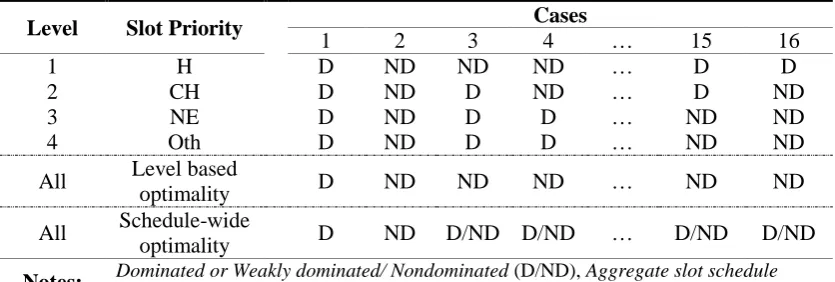
29

different decision entities. The table concludes that the only occasion to have a dominated level-based schedule-wide solution is to have dominated solutions for each of the levels (Proposition 2). Meanwhile, all other scenarios where there is at least one nondominated level, yield scheduling solutions which are level-based nondominated. To explain, even if schedule-wide objective values are not Pareto optimal, we do not know the priority that the decision maker(s) assign to each decision entity. Under this prism, even dominated solutions may be meaningful if the objective values of a level abide by the stakeholders’ needs.

However, given that the slot typologies are already prioritised by the hierarchical allocation, we may assume that the goal of the problem is the generation of all schedule-wide Pareto efficient solutions no matter what the Pareto status of the levels is. By building on previous arguments, we address this setting in Proposition 4.

PROPOSITION 4.

If a schedule-wide solution has for all nondominated points , then it is a nondominated aggregate (or schedule-wide) solution.

Proof. The result follows immediately by Definition 6 and Proposition 3.

Obviously, if a schedule-wide solution results for some , in level-based nondominated points , then it is not necessarily a Pareto optimal schedule-wide solution as there may exist other solutions resulting in the same or better objective values. Therefore, the set of level-based non-dominated solutions is a superset of the schedule-wide nondominated solutions. As a result, in order to parse the whole Pareto frontier, we have to generate the level-based Pareto frontier and then filter out dominated and weakly dominated schedule-wide (aggregate) solutions. This idea sparkled the conceptualisation of the solution algorithms devised in Section 5.2.

Level Slot Priority Cases

1 2 3 4 … 15 16

1 H D ND ND ND … D D

2 CH D ND D ND … D ND

3 NE D ND D D … ND ND

4 Oth D ND D D … ND ND

All Level based

optimality D ND ND ND … ND ND

All Schedule-wide

optimality D ND D/ND D/ND … D/ND D/ND

[image:29.595.89.507.178.319.2]

Notes: Dominated or Weakly dominated/ Nondominated_{considering all levels}_{(Schedule-wide)} (D/ND), Aggregate slot schedule

(30)

30

5.2. Solution algorithms

The solution approaches that we propose in this section are quasi-exact in the sense that they do not examine the entire decision space. They do so by taking advantage of the multi-level modelling in order to introduce additional bounds to the objectives of each level, hence considering additional policy rules. Moreover, they are hybrid as they employ a hierarchical approach similar to current practice (Ribeiro et al., 2018; Zografos et al., 2012), yet they allow compromise at the upper decision entities.

Algorithm 2 can employ any efficient tri-objective solution algorithm to find the non-dominated points for each level ( by allocating all the slots while considering in the objective functions

input:

output: Y # set of efficient multi-level trade-offs

1 # data structure with Pareto solutions of all levels

# data structure with utopian and negative utopian solutions of all levels for each objective

2 3

4 for repeat:

5 ; # Add the nondominated points of γ to Λ

6 for repeat:

7 for repeat:

8 ;

10 if then: # is the value of for level γ

11 ;

12 if

13 ;

15 # maximum values of objectives for level γ

16 # minimum values of objectives for level γ

17

18 Define: recursive ML-search ( )

19 if Γ then:

20 Stop; # termination of Algorithm 2

21 else:

25 ;

; 26

27 if then:

28 ;

29 if is feasible then:

30

31 return ;

32 recursive ML-search ( , = cap);

33 recursive ML-search (

Notes:

# stands for comments on the algorithmic process; in bold are common algorithmic functions; solution of the tri-objective slot allocation model with rolling capacity , priority requests , and equality constraints for the three objectives respectively

.

Multi objective, multi level, multi stakeholder considerations for airport slot allocation