Variable sized uncertainty and inverse problems in robust optimization

Variable-Sized Uncertainty and Inverse

Problems in Robust Optimization

Andr´

e Chassein

and Marc Goerigk

1_{Fachbereich Mathematik, Technische Universit¨at Kaiserslautern, 67653 Kaiserslautern,} Germany

2_{Department of Management Science, Lancaster University, Lancaster LA1 4YX, United} Kingdom

Abstract

In robust optimization, the general aim is to find a solution that performs well over a set of possible parameter outcomes, the so-called uncertainty set. In this paper, we assume that the uncertainty size is not fixed, and instead aim at finding a set of robust solutions that covers all possible uncertainty set outcomes. We refer to these problems as robust optimization with variable-sized uncertainty. We discuss how to construct smallest possible sets of min-max robust solutions and give bounds on their size.

A special case of this perspective is to analyze for which uncertainty sets a nom-inal solution ceases to be a robust solution, which amounts to an inverse robust optimization problem. We consider this problem with a min-max regret objective and present mixed-integer linear programming formulations that can be applied to construct suitable uncertainty sets.

Results on both variable-sized uncertainty and inverse problems are further sup-ported with experimental data.

Keywords: Robustness and sensitivity analysis; uncertainty sets; inverse optimiza-tion; optimization under uncertainty

1 Introduction

Robust optimization has become a vibrant field of research with fruitful practical appli-cations, of which several recent surveys give testimonial (see [ABV09, BTGN09, BBC11, GYd15, GS16, CG16b]). Two of the most widely used approaches to robust optimiza-tion are the so-called (absolute) min-max and min-max regret approaches (see, e.g., the

∗

Email: [email protected] †

classic book on the topic [KY97]). For some combinatorial optimization problem of the form

(P) min ctx:x∈ X ⊆ {0,1}n

with a set of feasible solutionsX, let U denote the set of all possible scenario outcomes for the objective function parameter c. Then the min-max counterpart of the problem is given as

min x∈Xmaxc∈U c

t_x

and the min-max regret counterpart is given as

min

x∈Xreg(x,U)

with

reg(x,U) := max c∈U c

t_x−opt(c)

whereopt(c) denotes the optimal objective value for problem (P) with objective c. In the recent literature, the problem of finding suitable sets U has come to the focus of attention, see [BS04, BPS04, BB09]. This acknowledges that the set U might not be “given” by a real-world practitioner, but is part of the responsibility of the operations researcher.

In this paper we consider the question how robust solutions change when the size of the uncertainty set changes. We call this approach variable-sized robust optimization and analyze how to find minimal sets of robust solutions that can be applied to any possible uncertainty sets. This way, the decision maker is presented with candidate solutions that are robust for different-sized uncertainty sets, and he can choose which suits him best. Results on this approach for min-max robust optimization are discussed in Section 2.

The notion of variable uncertainty has also been used in [Pos13], but is different to our approach: In their paper, the size of the uncertainty set depends on the solutionx, i.e., U =U(x), while we use size parameter that does not depend on x. Further related is the notion of parametric programming (see, e.g., [Car83]). Our approach can be seen as being a parametric robust optimization problem.

one can check which parts of a solution are particularly fragile, and strengthen them further. This approach is presented for min-max regret in Section 3.

Our paper closes with a conclusion and discussion of further research directions in Section 4.

2 Variable-Sized Min-Max Robust Optimization

In this section, we analyze how optimal robust solutions change when the size of the uncertainty set increases. We assume to have information about the midpoint (nominal) scenario ˆc, and the shape of the uncertainty set U. The actual size of the uncertainty set is assumed to be uncertain.

More formally, we assume that the uncertainty set is given in the form

Uλ ={ˆc}+λB

whereBis a convex set containing the origin and ˆc >0 is the midpoint of the uncertainty set. The parameter λ≥0 is an indicator for the size of the uncertainty set. Forλ= 0, we haveU0={ˆc}, i.e., the nominal problem, and forλ→ ∞ we obtain the extreme case

of complete uncertainty.

We consider the min-max robust optimization problem

min x∈Xmaxc∈Uλ

ctx. (P(λ))

The goal of variable-sized robust optimization is to compute a minimal set S ⊂ X such that for any λ≥0, S contains a solution that is optimal forP(λ). Note that for λ= 0, setS must contain a solution ˆx that is optimal for the nominal problem. By increasing

λ, we trace how this solution needs to change with increasing degree of uncertainty. Section 2 is structured as follows. In Section 2.1, we demonstrate the close relation between the variable-sized robust problem and a bicriteria optimization problem. We consider different shapes for setB in Section 2.2 and discuss the resulting variable-sized robust optimization problems. In Section 2.3, we transfer the general results of the previous section to the shortest path problem. We end the discussion of the shortest path problem with a case study.

2.1 Relation to Bicriteria Optimization

We reformulate the objective function ofP(λ):

max c∈Uλ

ctx= ˆctx+ max c∈λBc

t_{x= ˆc}t_{x+ max}

˜

c∈B λ˜c

t_{x= ˆc}t_x+λmax

˜

c∈B ˜c t_x=f

1(x) +λf2(x)

where f1(x) = ˆctx and f2(x) = maxc∈Bctx. Note that both functions are convex. It is immediate that the variable-sized robust optimization problem is closely related to the bicriteria optimization problem:

min x∈X

f1(x)

We define the map F : X → _R2

+, F(x) = (f1(x), f2(x))t which maps every feasible

solution in the objective space. Further, we define the polytope V = conv({F(x) :x ∈ X }) +R2+. We call a solutionx∈ X anefficient extreme solutionifF(x) is a vertex ofV.

Denote the set of all efficient extreme solutions withE. We call two different solutions

x6=x0 equivalent ifF(x) =F(x0). Let Emin ⊂ E be a maximal subset such that no two

solutions of Emin are equivalent. The next lemma gives the direct relation betweenEmin

and the variable-sized robust optimization problem.

Lemma 1. E_min is a solution of the variable sized robust optimization problem. Proof. We need to prove two properties:

(I) For everyλ≥0 there exists a solution inEmin which is optimal forP(λ).

(II) E_min is a smallest possible set with property (I).

(I) Letλ≥0 be fixed. We transfer the problemP(λ) in the objective space. The optimal value of P(λ) is equal to the optimal value of problem O(λ) since each optimal solution of this problem is a vertex ofV.

min

v∈V v1+λv2 (O(λ))

Let v∗ be the optimal solution ofO(λ). By definition, E_min contains a solution x∗ with

F(x) =v∗, i.e., an optimal solution for P(λ).

(II) Note that there is a one-to-one correspondence between vertices ofV and solutions in E_min. Since for each vertex v0 of V a λ0 ≥0 exists such that v0 is optimal for O(λ), it follows that E_min is indeed minimal. Note that it is important to ensure that E_min

contains no equivalent solutions.

Different methods are known to computeEmin. The complexity of these methods depends

linearly on the size of Emin. To find an additional efficient extreme solution a weighted

sum problem of the form minx∈Xf1(x) +λf2(x) needs to be solved. In the following, we

denote by T the time which is necessary to solve the nominal problem minx∈XcTx and

by T0 the time that is necessary to solve a weighted sum problem. Note that iff2(x) is

linear inx,O(T0) =O(T). We restate the following well known result (see e.g. [Mor86]).

Lemma 2. Emin can be computed in O(|Emin|T0).

Using Lemma 1, we can transfer this result to the variable-sized robust problem.

Theorem 3. The variable-sized robust problem can be solved in O(|E_min|T0).

2.2 General Results

We assume that B is the unit ball of some norm. An overview of different norms and the corresponding functions maxc∈Uλc

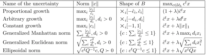
Name of the uncertainty Normkck Shape ofB maxc∈Uλc

t_x Proportional growth maxi |c_ˆci_i|

×

di , di>0

×

t_x+λdt_x Constant growth maxi|ci|

×

Generalized Manhattan norm P

i

|ci|

di , di >0 {c: P

i

|ci|

di ≤1} ˆc

t_x+λmaxid ixi Generalized Euclidean norm

q P

i c2

i

di, di >0 {c: P

i c2

i

di ≤1} ˆc

t_x+λqP

idix2i Ellipsoidal norm pct_Q−1_{c, Q0 {c:c}t_Q−1_{c≤1} ˆc}t_x+λp

xt_Qx

Table 1: Overview of different shapes for the uncertainty setU_λ.

information about different shapes for uncertainty sets and the resulting robust objective function we refer to [BTdHV15].

We add to the first three cases the suffix growth since the setsB have the form of a hyper box and, hence, each cost coefficient grows linear inλand independent from the other coefficients. For proportional growth the coefficients ci grow proportional to the nominal cost vector ˆc, for arbitrary growth each cost coefficient ci has its own growth speed di, and for constant growth all cost coefficients grow at unit speed. For the last three cases setB has a more complex structure, we name them by the norm definingB. The generalized Euclidean norm leads to an ellipsoidal uncertainty set which is axis aligned. Whereas the more general ellipsoidal norm leads to an ellipsoidal uncertainty set with arbitrary rotation.

For proportional growth it is immediate that a nominal solution ˆxwhich is optimal for cost vector ˆcis optimal for anyλ≥0. Hence, the optimal solution for the variable-sized robust optimization problem consists of a single element,S ={xˆ}.

Note that the case of constant growth leads to the concept ofL1-regularization, which

is closely related to the well known Lasso method (we refer to [BBC11] for a discussion of Lasso and robust optimization).

Consider function f2(x) = maxc∈BcTx for constant growth (f2(x) = kxk1) and for

the generalized Manhattan norm (f2(x) = maxidixi). Since we consider combinatorial optimization problems we conclude that|{f2(x) :x∈ X }| ≤nfor both cases. Note that

this gives an direct bound for the number of efficient extreme solutions|Emin| ≤n. We

summarize these findings in the next two theorems.

Theorem 4. The variable-sized robust optimization problem with constant growth can be solved in O(nT) and |S| ≤n.

Theorem 5. The variable-sized robust optimization problem with the generalized Man-hattan norm can be solved in O(nT0) and |S| ≤n.

Lemma 6. Let f1(x), f2(x)≥0 ∀x∈ X. Each efficient extreme solution of

min x∈X

f1(x) p

f2(x)

(P1)

is an efficient extreme solution of

min x∈X

f1(x)

f2(x)

. (P2)

Proof. We define the mapscd:X →R2, cd(x) = (f1(x), f2(x)) andcd0 :X →R2, cd0(x) = (f1(x),

p

f2(x)). Further denote by Cmin = minx∈Xf1(x) and Dmin = minx∈Xf2(x).

Let x0 be an efficient extreme solution of P1. If cd(x0)1 =Cmin orcd(x0)2 =Dmin, it is

straightforward to show thatx0 is also efficient extreme forP2. Hence, we assume in the

following thatcd(x0)1 > Cminandcd(x0)2 > Dmin. We assume, for the sake of

contradic-tion, that x0 is not an efficient extreme solution ofP2. This means that two other

solu-tionsx1, x2∈ X and anα∈[0,1] exists such thatαcd(x1)1+(1−α)cd(x2)1=cd(x0)1 and

αcd(x1)2+ (1−α)cd(x2)2≤cd(x0)2. It follows thatαcd0(x1)1+ (1−α)cd0(x2)1 =cd0(x0)1

and αcd0(x1)2+ (1−α)cd0(x2)2 ≤ p

αcd(x1)2+ (1−α)cd(x2)2 ≤ p

cd(x0₎

2 =cd0(x0)2,

since the square root is a concave and monotone function. This yields the desired con-tradiction, sincex0 is an efficient extreme solution for P1.

Note that instead of using the square root function on f2(x) in P1, the proof can be

extended to any increasing, concave function. Observe that ˆctx+λP

idix2i = ˆctx+λdtx, since we consider combinatorial optimization problems. Hence, using Lemma 6 we can solve the variable-sized robust optimization problem with generalized Euclidean norm by computing the set of extreme efficient solutions for the bicriteria optimization problem with objective functions ˆctx and dtx. In this way may found some solutions which are not extreme efficient for the original bicriteria optimization problem with objective functions ˆctx and √dt_{x. After these solutions are removed, we have found the solution} to the variable-sized robust optimization problem with generalized Euclidean norm.

The same approach can be applied in the case of an ellipsoidal norm. In this case, the alternative bicriteria optimization problem has the objective functions ˆcTx and xtQx.

2.3 Application to the Shortest Path Problem

In this section, we transfer the general results from the last section to the shortest path problem. The problem is defined on a graph G = (V, E) with N nodes and M edges. We denote by P the set of all paths from start node s∈ V to end note t ∈ V. For a pathP ∈ P, we writec(P) =P

2.3.1 Constant growth

We consider in more detail the implications of Theorem 4 to the shortest path problem. The corresponding bicriteria optimization problem is

min P∈P

ˆ

c(P)

|P|

Note that it suffices to consider simple paths for this bicriteria optimization problem as we assume that all edge costs are positive. As each simple path contains at most N

edges |P| ∈ {1, . . . , N}, the cardinality of E_min is bounded by N. The computation of this set can be done at once using a labeling algorithm that stores for each pathQfrom

s to v the cost of the path ˆc(Q) and the number of edges contained in the path |Q|. Note that at each node at mostN labels needs to be stored, this ensures the polynomial running time of the labeling algorithm. An alternative approach is to use an efficient procedure to computeEmin (see [Mor86]). Each weighted sum computation corresponds

to a shortest path problem.

Theorem 7. The variable-sized robust shortest path problem for a graph G = (V, E) with |V|=N and |E|=M with constant growth can be solved in O(N M +N2log(N)) and |S| ≤N.

Proof. The nominal problem can be solved by Dijkstra’s algorithm inO(M+Nlog(N)).

2.3.2 Generalized Manhattan norm

We consider in more detail the implications of Theorem 5 to the shortest path problem. The corresponding bicriteria optimization problem is

min P∈P

ˆ

c(P) maxe∈Pde

The setE_minis bounded by the number of different values ofde,e∈E, which is bounded byM. The computation of this set can be done at once using a labeling algorithm that stores for each pathQfromstovthe cost of the path ˆc(Q) and the most expensive edge of Q with respect to cost function d. Note that at each node at most M labels needs to be stored, this ensures the polynomial running time of the labeling algorithm. An alternative approach is to use an efficient procedure to computeEmin(see [Mor86]). If we

use Dijkstra’s algorithm to solve the nominal problem we obtain the following running time.

Theorem 8. The variable-sized robust shortest path problem for a graph G = (V, E) with |V| = N and |E| = M with the generalized Manhattan norm can be solved in

O(M2+N Mlog(N))and |S| ≤M.

2.3.3 Arbitrary Growth

Carstensen presents in her PhD thesis [Car83] bicriteria shortest path problems with two linear objective functions in which |E_min| ∈ 2Ω(log2(N)), which is not polynomial in

N. Further, she proved for acylic graphs that K ∈O(nlog(n)_{) which is subexponential.}

Note that this result can directly been applied to the variable-sized robust shortest path problem with arbitrary growth.

Theorem 9. The variable-sized robust shortest path problem on acyclic graphs with arbitrary growth can be solved in subexponential time and |S| is also subexponential. If we further restrict the graph class of G, the following results can be obtained.

Theorem 10. Let G be a series-parallel graph with N nodes and M arcs. Then, K ≤

M−N+2, and the variable-sized robust shortest path problem can be solved in polynomial time.

Proof. We do a proof by an induction over the depth D(G) of the decomposition tree of graph G. For the induction start, note that ifD(G) = 1, G only consists of a single edge. Hence, there exists exactly one s−t path, which is obviously also an extreme efficient solution. Therefore, K = 1. There are two nodes and one arc, i.e., N = 2 and

M = 1. Hence, K≤M −N + 2 holds.

We distinguish two cases for the induction step:

Case 1: Gis a parallel composition of two series-parallel graphsG1 and G2.

Every path that is an extreme efficient solution for the shortest path problem in graph

Gis then either completely contained inG1 orG2, and, hence, must also be an extreme

efficient solution of the shortest path instance described by G1 or G2. Therefore, the

number of extreme efficient paths in G1 plus the number of extreme efficient paths

in G2 is an upper bound for the number of extreme efficient paths in G. Note that

D(G1) < D(G) and D(G2) < D(G). Hence, we can apply the induction hypothesis to

G1andG2. Denote byKi the number of extreme efficient paths inGi, byNi the number of nodes, and by Mi the number of edges of Gi fori= 1,2. We have that

K ≤K1+K2≤(M1−N1+ 2) + (M2−N2+ 2)

=M1+M2−(N1+N2−2) + 2 =M−N+ 2

Case 2: Gis a series composition of two series-parallel graphs G1 and G2.

Note that for every extreme efficient path, there exists an open interval (λ, λ) such that this path is the unique optimal path with respect to the weight functionλc+ (1−λ)dfor all λ∈(λ, λ). Hence, we can find an ordering of all extreme efficient paths with respect to the λ values. Note that all extreme efficient paths in G must consist of extreme efficient paths ofG1 and G2. The extreme paths of Gcan be obtained in the following

way. We start with the shortest paths with respect tocinG1and G2 and combine these

changes. This change will define a new extreme path. We continue until all extreme paths ofG1 andG2are contained in at least one extreme path. Note thatD(G1)< D(G)

andD(G2)< D(G). Hence, we can apply the induction hypothesis to G1 andG2. Note

that the number of changes is bounded by the number of extreme efficient paths minus 1. Since, for every such change, we get one additional extreme efficient path, we get in total

K ≤1 + (M1−N1+ 2−1) + (M2−N2+ 2−1)

=M1+M2−(N1+N2−1) + 2

=M−N + 2.

Using a similar proof technique we can bound K also for layered graphs. A layered graph consists of a source nodesand a destination nodetand`layers, each layer consists of w nodes. Node s is fully connected to the first layer, the nodes of the ith layer are fully connected to the nodes of the (i+ 1)th layer, and the last layer is fully connected to nodet.

Theorem 11. Let G be a layered graph with ` layers and width w. Then, K ≤

(2w)dlog(`+1)e.

Proof. Without loss of generality we can assume that`= 2k−1 for some k∈_N. Then, the claimed bound simplifies to K ≤ (2w)k. Denote by E(t) the number of extreme efficient paths in G with 2t_{−1 many layers. The base case is given by E(0) = 1, since} the corresponding graph consists of a single edge. To boundE(k) we make the following observation. Eachs−tpath contains a single node j ∈[w] from the middle layer (the middle layer is the (2k−1 −1)th layer). Hence, we can separate all s−t paths into w

disjoint different classes. Let Ej be the number of extreme efficient solutions in each classj∈[w]. The same arguments as in Case 2 in the proof of Theorem 10 can be used to show that Ej is at most the number of extreme efficient paths from sto j plus the number of extreme efficient paths from j to t minus 1. Observe further that all paths from s to a node j on the middle layer and all paths from j to t are contained in a layered graph with widthw and 2k−1−1 layers. Using these arguments we obtain the bound: E(k)≤w(2E(k−1)−1). Using this bound we can derive the claimed bound

K=E(k)≤w(2E(k−1)−1)≤2wE(k−1)≤(2w)kE(k−k) = (2w)k

Remark: The bound proved in Theorem 11 is subexponential for general layered graphs. But if ` orw is assumed to be fixed, the bound is polynomial: Since N ≈`w, w ≈ N

` and `≈ N

w, we have for ` fixed K ∈ O ( N

`)

log(`)

∈ O Nlog(`)

and, conversely, for w

fixedK ∈O(2w)log(Nw)

∈O Nlog(w)+1

Name of the uncertainty Graph type Computation Time Proportional growth General O(T)

Constant growth General O(N T) Generalized Manhattan norm General O(M T)

Arbitrary growth Acylic Subexponential Arbitrary growth Series-parallel O(M T)

Arbitrary growth Layered O((2w)dlog(`+1)eT)

Table 2: Results for the variable-sized robust shortest path problem.

2.3.4 Ellipsoidal Norm

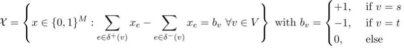
The feasible set of the shortest path problem, i.e. all incidence vectors of s-t paths can be represented in the following way

X =







x∈ {0,1}M : X e∈δ+_(v)

xe−

X

e∈δ−_(v)

xe=bv ∀v∈V







withbv =



 

 

+1, ifv=s

−1, ifv=t

0, else

where δ+(v)(δ−(v)) is the set of are all edges leaving (entering) v. Note that the constraints defining X do not forbid cycles for the s-t paths. Nevertheless, we can use this set for the optimization problem, since all solutions containing cycles are suboptimal. The weighted sum problem which needs to be solved to compute the set of extreme efficient solutions can be represented by the following mixed integer second order cone programming problem.

min ctx+r

s.t. xtQx≤r2 x∈ X

The computational complexity of this problem is NP-complete and even APX-hard as shown in [RCH+16]. Nevertheless, real world instances can be solved exactly using modern solvers.

Before we conclude the section with a case study of the variable-sized robust shortest path problem with ellipsoidal uncertainty, we present an overview of the different results obtained in this section in Table 2.

2.3.5 Case Study

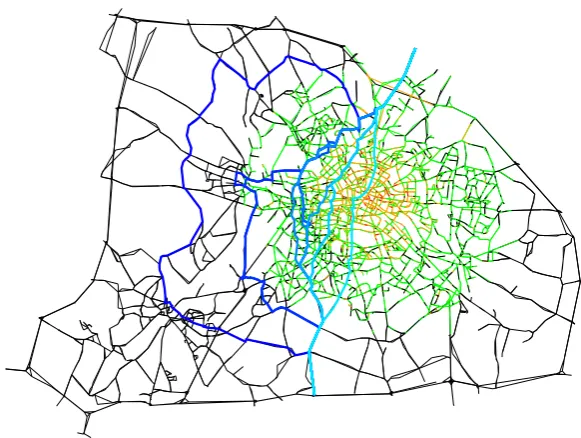
In this case study we consider the problem of finding a path through Berlin, Germany. We use a road network of Berlin which consists of 12,100 nodes and 19,570 edges. The data set was also used in [JMSSM05], and taken from the collection [BG16]. We use the following probabilistic model to describe the uncertain travel times of each road segment.

Figure 1: Berlin case study - Solution of the variable-sized robust shortest path prob-lem. The color of each edge indicates the degree of uncertainty that affects this edge: Black almost no uncertainty, green small uncertainty, orange -medium uncertainty, and red - high uncertainty. The 11 different paths found as solution of the robust problem are drawn in blue: Light blue represents the nominal solution and dark blue the most robust solution.

where ξ ∼ N(0, I) is a k-dimensional random vector which is multivariate normal dis-tributed, L∈_RM×k_{, and ˆc is taken from the data set. Under this assumption c is also} multivariate normally distributed with mean ˆc and variance LLt. Note that the most likely realization of c form an ellipsoid. Protecting against these realizations we obtain an ellipsoidal uncertainty set.

Entries of L are chosen such that the road segments in the center of Berlin tend to be affected by more uncertainty. We compute all solutions to the variable-sized robust problem, solving the resulting mixed integer second order cone programming problem with Cplex v.12.6. Computation times were less than three minutes on a desktop computer with an Intel quad core i5-3470 processor, running at 3.20 GHz. The solution of the variable-sized robust problem contains 11 different paths. These paths are shown in Figure 1.

30000 40000 50000 60000 70000 80000 90000 100000

0 20 40 60 80 100 120 140 160

Nominal cost

Uncertainty level λ

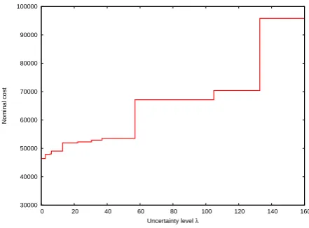
Figure 2: Berlin case study - Robustness chart. The curve indicates the nominal cost of the robust solution for some fixed uncertainty level λ.

In the robustness chart (see Figure 2) it is shown how the nominal cost (ˆctx) of the different compromise solution increase with an increasing level of uncertainty (λ). The chart provides the decision maker with detailed information about the cost of considering larger levels of uncertainty, and shows for how long solutions remain optimal.

We find that variable-sized robust optimization gives a more thorough assessment of an uncertain optimization problem than classic robust approaches would be able to do, while also remaining suitable with regards to computational effort.

3 Inverse Min-Max Regret Robustness

3.1 General Discussion

Having considered variable-sized approaches in the previous section, we now consider the special case of analyzing the nominal solution only.

Let ˆxbe an optimal solution to the nominal problem (P) with costs ˆc, i.e.,

ˆ

x∈arg min{cˆtx:x∈ X }

Note that in this case, ˆx is also an optimizer of the min-max and min-max regret coun-terparts for the singleton set ˆU ={ˆc}, i.e.,

ˆ

x∈arg min

max c∈Uˆ

ctx:x∈ X

and ˆx∈arg minnreg(x,Uˆ) :x∈ Xo.

Firstly, the “size of an uncertainty set” needs to be specified. In this section, we discuss two approaches:

• For uncertainty sets of the form

U(λ) ={c:ci∈[(1−λ)ˆci,(1 +λ)ˆci]},

the parameter λ ∈ [0,1] specifies the uncertainty size, with U(0) = ˆU. We call these setsregular interval sets. Note that this corresponds to proportional growth in the previous section.

• Forgeneral interval uncertainty sets

U(d+, d−) ={c:ci ∈[ˆci−d−i ,cˆi+d+i ]∀i∈[n]}, the size ofU(d+, d−) is the length of intervals |U(d+, d−)|:=P

i∈[n]d

−

i +d

+

i , with

|U |ˆ =|Uˆ(0,0)|= 0.

For general uncertainty sets, there are different ways to distribute a fixed amount of slack d− ≥ 0,d+ ≥ 0, all resulting in the same uncertainty size. Depending on the application, it may be useful to use upper boundsd−≤M− and d+≤M+.

Secondly, one can either look for the uncertainty set of the smallest possible size for which ˆx is not optimal for the resulting robust objective function; or one can look for the largest possible uncertainty set for which ˆx is still optimal in the robust sense. We refer to these approaches as worst-case or best-case inverse robustness, respectively. Our approach may also be used to choose the most robust of several candidate solutions. The problem of finding the best robust solution in a lexicographic sense has also been considered in a different setting in [IT13].

In Section 3.2, we discuss regular interval uncertainty sets, while Section 3.3 presents results on general interval sets.

3.2 Regular Interval Uncertainty Sets

3.2.1 Problem Structure

Note thatreg(x, λ) :=reg(x,U(λ)) is a monotonically increasing function inλfor allx. The following calculations show that reg(x, λ) is a piecewise-linear function in λ.

reg(x, λ) = max c∈U(λ)

ctx−min y∈Xc

t_y

= max

y∈X cmax∈U(λ)c

t_x−ct_y

= max y∈X c(x, λ)

t_{x−c(x, λ)}t_y

= max

y∈X(1 +λ)c

t_x−X

i∈[n]

Here we use that the scenario c ∈ U(λ) maximizing reg(x, λ) is given by c(x, λ)i =

ci(1−λ+ 2λxi). Observe that c(x, λ)ixi = (1 +λ)cixi.

This gives rise to the question: Is there also any difference between worst-case and best-case inverse robustness for regular interval sets? That is, is it possible that a situation occurs as shown in Figure 3, where the regret of the nominal solution becomes larger than the regret of another solution for some λ1, but for another λ2 > λ1, this

situation is again reversed? Here, the best-case robustness approach would yieldλ=λ2

as the largest value of λfor which ˆx is an optimal regret solution. However, the worst-case approach would give λ1 as the smallest value for which ˆx is not regret optimal.

Such a situation can indeed occur, as the following example demonstrates.

Figure 3: Comparison of the regret of two solutions ˆxand x0 for different values ofλ.

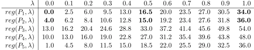
Example 12. Consider the shortest path instance presented in Figure 4. A feasible path starts at node1 and ends at node 6.

Figure 4: A sample shortest path instance with regular interval sets. The label over each edge specifies the midpoint of this edge ˆci.

We describe paths by the succession of nodes they visit. There are five feasible paths in the graph, P1 = (1,2,3,6), P2 = (1,2,4,5,6), P3 = (1,2,4,5,3,6), P4 = (1,4,5,3,6)

λ 0.0 0.1 0.2 0.3 0.4 0.5 0.6 0.7 0.8 0.9 1.0

reg(P1, λ) 0.0 2.5 6.0 9.5 13.0 16.5 20.0 23.5 27.0 30.5 34.0

reg(P2, λ) 4.0 6.2 8.4 10.6 12.8 15.0 19.2 23.4 27.6 31.8 36.0

reg(P3, λ) 13.0 16.2 20.4 24.6 28.8 33.0 37.2 41.4 45.6 49.8 54.0

reg(P4, λ) 10.0 13.0 16.0 19.0 22.8 27.0 31.2 35.4 39.6 43.8 48.0

reg(P5, λ) 1.0 4.5 8.0 11.5 15.0 18.5 22.0 25.5 29.0 32.5 36.0

Table 3: Regret of paths in Figure 4 depending onλ.

A unique minimizer of the nominal scenario (i.e., λ= 0) is the path P1 with a regret

of zero, while path P2 has a regret of four. For λ= 0.5, the regret of path P1 becomes

16.5, but is only 15 for path P2. Finally, for λ= 1, path P1 has a regret of 34, but path

P2 has a regret of 36, i.e., path P2 has the better regret for λ= 0.5, but not for λ= 0

and λ= 1. Also, P1 is indeed the path with the smallest regret for λ= 1.

Note how such an example is in contrast to variable-sized min-max robust optimiza-tion, where a solution that ceases to be optimal for some value λ will not be optimal again for another value λ0 > λ. The above example can also be extended such that a path is optimal on an arbitrary number of disjoint intervals ofλ.

In the following, we analyze the best-case setting in Section 3.2.2 and the worst-case setting in Section 3.2.3. We only focus on analyzing the nominal solution; an extension how this approach can be used to solve the complete variable-sized problem is given in Section 3.2.4.

3.2.2 Best-Case Inverse Robustness

The best-case inverse problem we consider here can be summarized as: Given some solution ˆx, what is the largest amount of uncertainty that can be added such that ˆx is still optimal for the resulting min-max regret problem? The method we present in the following to answer this question can in fact be applied to any solution x ∈ X, in the sense that we find the largest set U(λ) such that x is an optimal regret solution, if it exists.

More formally, the best-case inverse problem we consider here is given as:

max λ

s.t. reg(ˆx, λ)≤reg(˜x, λ) ∀x˜∈ X

λ∈[0,1] wherereg(x, λ) = maxc∈Uλ c

t_x−opt(c)

.

duality is an important tool in classic min-max regret problems, as it allows a compact problem formulation [ABV09]. As an example, we consider the assignment problem in the following. The nominal problem is given by

min X i∈[n]

X

j∈[n]

ˆ

cijxij

s.t. X i∈[n]

xij = 1 ∀j∈[n]

X

j∈[n]

xij = 1 ∀i∈[n]

xij ∈ {0,1} ∀i, j∈[n]

Using thatreg(x, λ) =ct(x)x−opt(c(x)) with

cij(x) =

(

(1 +λ)ˆcij ifxij = 1, (1−λ)ˆcij else

and dualizing the inner optimization problem, we find a compact formulation of the min-max regret problem as follows:

min X i∈[n]

X

j∈[n]

(1 +λ)ˆcijxij−

X

i∈[n]

(ui+vi)

s.t. ui+vj ≤(1−λ)ˆcij + 2λˆcxij ∀i, j∈[n]

X

i∈[n]

xij = 1 ∀j∈[n]

X

j∈[n]

xij = 1 ∀i∈[n]

xij ∈ {0,1} ∀i, j∈[n]

ui, vi≷0 ∀i∈[n]

We now re-consider the inverse problem. Note that to reformulate the constraints

reg(ˆx, λ)≤reg(˜x, λ) ∀x˜∈ X

we can use the same duality approach for the left-hand side (as an optimal solution aims at having this side as small as possible), but not for the right-hand side (which should be as large as possible). Instead, for each ˜x∈ X, we need to provide a primal solution. Enumerating all possible solutions inX as ˜xk,k∈[|X |], the inverse problem can hence be reformulated as

max λ (1)

s.t. X i,j∈[n]

(1 +λ)ˆcijxˆij−

X

i∈[n]

≤ X

i,j∈[n]

(1 +λ)ˆcijx˜kij −

X

i,j∈[n]

((1−λ)ˆcij + 2λˆcijx˜kij)xkij ∀k∈[|X |] (2)

ui+vj ≤(1−λ)ˆcij+ 2λcˆijxˆij ∀i, j∈[n] (3)

λ∈[0,1] (4)

ui, vi ≷0 ∀i∈[n] (5)

xk∈ X ∀k∈[|X |] (6)

Here, the objective function (1) is to maximize the size of the uncertainty set λ. Con-straints (2) model that the regret of ˆx needs to be at most as large as the regret of all possible alternative solutions ˜xk. To calculate the regret of these solutions, additional solutions xk are required. The duality constraints in (3) ensure that the regret of ˆx is calculated correctly.

To solve this problem, not all variables and constraints need to be included from the beginning. Instead, we can generate them during the solution process of the master prob-lem by solving subprobprob-lems that aim at minimizing the right-hand side of Constraint (2). This is a classic min-max regret problem again.

To resolve the non-linearity between xkand λ, we use additional variablesy_ijk :=λxk_ij. The resulting mixed-integer program is then given as:

max λ (7)

s.t. X i,j∈[n]

(1 +λ)ˆcijxˆij −

X

i∈[n]

(ui+vi) (8)

≤ X

i,j∈[n]

(1 +λ)ˆcijx˜kij −

X

i,j∈[n]

(ˆcijxkij+ (2˜xkij −1)ˆcijykij) ∀k∈[|X |] (9)

ui+vj ≤(1−λ)ˆcij + 2λˆcijxˆij ∀i, j∈[n] (10) 0≤y_ijk ≤λ ∀i, j∈[n], k∈[|X |] (11)

λ+xk_ij−1≤yk_ij ≤xk_ij ∀i, j∈[n], k∈[|X |] (12)

λ∈[0,1] (13)

ui, vi≷0 ∀i∈[n] (14)

y_ijk ≥0 ∀i, j∈[n], k∈[|X |] (15)

xk ∈ X ∀k∈[|X |] (16)

For a more general formulation, which is not restricted to the assignment problem, let us assume that X = {x : Ax ≥ b, x ∈ {0,1}n_{} with A ∈}

Rm×n and b ∈ Rm, and that strong duality holds. Then the min-max regret problem with interval sets U_λ can be formulated as

min

x∈X,u∈Y (1 +λ)ˆcx−b

t_u

min-max regret, we can substitute Constraint (9) for

X

i∈[n]

(1 +λ)ˆcixˆi−btu≤

X

i∈[n]

(1 +λ)ˆcix˜ki −

X

i∈[n]

(ˆcixki + (2˜xki −1)ˆciyik) ∀k∈[|X |]

and Constraints (10) for

(Atu)i ≤(1−λ)ˆci+ 2λcˆixˆi ∀i∈[n] with dual variablesui≥0 for alli∈[m].

We conclude this section by briefly considering the case where the original problem (P) does not have zero duality gap. In this case, we rewrite the constraints

reg(ˆx, λ)≤reg(˜xk, λ) ∀k∈[|X |] as

X

i∈[n]

(1 +λ)ˆcixˆi−

X

i∈[n]

((1−λ)ˆci+ 2λcˆixˆi) ¯x`i

≤X

i∈[n]

(1 +λ)ˆcix˜ki −

X

i∈[n]

((1−λ)ˆci+ 2λˆcix˜ki)xki ∀k, `∈[|X |]

i.e., we compute the regret on both sides of the inequality by using all primal solutions as comparison. As before, variables and constraints can be generated iteratively during the solution process. To find the next solution ¯x`, only a problem (P) or the original type needs to be solved.

3.2.3 Worst-Case Inverse Robustness

We now consider the worst-case inverse problem, which may be summarized as: Given some solution ˆx, what is the smallest amount of uncertainty that needs to be added such that ˆx is not optimal for the resulting min-max regret problem anymore?

More formally, the problem we consider can be denoted as:

minλ (17)

s.t. reg(ˆx, λ)≥reg(˜x, λ) +ε (18)

λ∈[0,1] (19)

˜

x∈ X (20)

where ε is a small constant, i.e., we need to find an uncertainty parameter λ and an alternative solution ˜xsuch that the regret of ˜xis at least better by εthan the regret of ˆ

x.

As in the previous section, we use the assignment problem as an example how to rewrite this problem in compact form. As an optimal solution will aim at having the right-hand side of Constraint (37) as small as possible, we use strong duality to write:

s.t. reg(ˆx, λ)≥ X

i,j∈[n]

(1 +λ)ˆcijx˜ij −

X

i∈[n]

(ui+vi) +ε

ui+vj ≤(1−λ)ˆcij + 2λˆcijx˜ij ∀i, j∈[n]

λ∈[0,1] ˜

x∈ X

For the left-hand side of Constraint (18), we need to include an additional primal solution

x0 as an optimal solution for the worst-case scenario of ˆx. Linearizing the resulting products by setting yij := λx0ij and βij := λx˜ij, the resulting problem formulation is then:

min λ (21)

s.t. X i,j∈[n]

(1 +λ)ˆcijxˆij −

X

i,j∈[n]

(ˆcijx0ij+ (2ˆxij −1)ˆcijyij) (22)

≥ X

i,j∈[n]

(ˆcijx˜ij+ ˆcijβij)−

X

i∈[n]

(ui+vi) +ε (23)

ui+vj ≤(1−λ)ˆcij + 2ˆcijβij ∀i, j∈[n] (24)

0≤yij ≤λ ∀i, j∈[n] (25)

λ+x0_ij−1≤yij ≤λ ∀i, j∈[n] (26)

0≤βij ≤λ ∀i, j∈[n] (27)

λ+ ˜xij−1≤βij ≤λ ∀i, j∈[n] (28)

X

i∈[n]

x0_ij = 1 ∀i∈[n] (29)

X

j∈[n]

x0_ij = 1 ∀j∈[n] (30)

X

i∈[n]

˜

xij = 1 ∀i∈[n] (31)

X

j∈[n]

˜

xij = 1 ∀j∈[n] (32)

λ∈[0,1] (33)

x0_ij,x˜ij ∈ {0,1} ∀i, j∈[n] (34)

yij, βij ∈[0,1] ∀i, j∈[n] (35)

Note that this formulation has polynomially many constraints and variables, and thus can be attempted to be solved without an iterative procedure. In general, for a problem with X ={x :Ax≥b, x∈ {0,1}n_{} and the strong duality property, we can substitute} Constraint (23) for

X

i∈[n]

(1 +λ)ˆcixˆi−

X

i∈[n]

(ˆcix0i+ (2ˆxi−1)ˆciyi)≥

X

i∈[n]

and Constraints (24) for

(Atu)i ≤(1−λ)ˆci+ 2ˆciβi ∀i∈[n] with dual variablesui≥0 for alli∈[m].

In the case that problem (P) does not have a zero duality gap, we propose to follow a similar strategy as in Section 3.2.2. That is, we consider constraints

X

i∈[n]

(1 +λ)ˆcixˆi−

X

i∈[n]

(ˆcix0i+ (2ˆxi−1)ˆciyi)

≥ X

i∈[n]

(1 +λ)ˆcix˜i−

X

i∈[n]

((1−λ)ˆci+ 2λcˆix˜i)xki +ε ∀k∈[|X |]

and generate them iteratively in a constraint relaxation procedure. Note that no addi-tional variables are required.

3.2.4 Extension to the Variable-Sized Problem

Recall the relationship between the variable-sized min-max robust optimization problem and a bicriteria optimization problem discussed in Section 2, which allowed us to effi-ciently solve the problem. Unfortunately, such a connection cannot be derived for the variable-sized min-max regret robust optimization problem. Nevertheless, it is possible to compute a solution for the problem, i.e. a minimal set S such that for each λ∈[0,1] there exists a solution x ∈ S which is optimal for the min-max regret problem with uncertainty setU(λ). In the following, we sketch a method that can be used to compute

S.

Let x be a fixed solution. Recall that reg(x, λ) is a piecewise linear function in λ

(see Figure 3). Each linear part of this function corresponds to a solution of the classic optimization problems. Hence, the function can be computed by solving a sequence of classic optimization problem. For an detailed description of the algorithm which computes the piecewise linear function reg(x, λ) we refer to [CG16a]. A brute force method to solve the variable-sized problem is to compute for each solution x ∈ X the functionreg(x, λ). Then, we form the minimum over all these functions, i.e. we compute

F(λ) = minx∈Xreg(x, λ). Note that F is again piecewise linear. Given F, to obtain

solution S of the variable-sized optimization problem is straightforward. Simply chose all solutions which contribute to function F. We can improve this brute force method by iteratively generating function F.

We start with some arbitrary solution x0. We computereg(x0, λ) and set X0={x0}.

Further, we defineF0(λ) = minx∈X0reg(x, λ). The idea is to iteratively increase set X0 until F0(λ) = F(λ) for all λ ∈ [0,1]. To do this, we pick an interval [λ1, λ2] ⊂ [0,1]

for which F0 is linear. Assume thatF0(λ) = mλ+b for all λ∈[λ1, λ2]. To verify that

reg(x, λ)≥mλ+b. This can be done by solving the following optimization problem. min reg(x, λ)−mλ−b

x∈ X

λ∈[λ1, λ2]

Denote by x0 the optimal solution and by f0 the optimal value of this optimization problem. Note that this problem can be transformed to a mixed integer programming problem using strong duality and the same linearization technique as used for prob-lem (7)–(16). Iff0≥0, we have verified thatF0(λ) =F(λ) for allλ∈[λ1, λ2]. Iff0 <0,

we add solution x0 to X0_{, compute reg(x}0_{, λ), and update F}0_{. In both cases, we pick}

a new interval for which we have not yet verified that F0(λ) = F(λ). Note that this process terminates after a finite number of steps with F0=F.

3.3 General Interval Uncertainty Sets

3.3.1 Best-Case Inverse Robustness

We now consider consider general interval uncertainty, where the size of the uncertainty is the summed length of intervals, i.e., the best-case inverse problem we consider here is given as:

max X

i∈[n]

d+_i +d−_i

s.t. reg(ˆx, d+, d−)≤reg(˜x, d+, d−) ∀x˜∈ X

d+_i ∈[0, M_i+] ∀i∈[n]

d−_i ∈[0, M_i−] ∀i∈[n]

whereM_i+,M_i− denote the maximum possible deviations in each coefficient, and

reg(x, d+, d−) = max c∈U(d+_,d−₎c

t_x−opt(c).

By settingM_i+ = 0 orM_i−= 0 for some indexi, we can model that this coefficient may not deviate in the respective direction.

We first consider this setting with the unconstrained combinatorial optimization prob-lem, where X ={0,1}n_.

Let ˆx be optimal for ˆc. Note that for some fixed c, an optimal solution is to pack all items with negative costs. Therefore, we assume

ˆ

xi=

(

1 if ˆci≤0 0 else

Lemma 13. (See [CG17]) LetU =×_i∈[n][ˆci−di,cˆi+di]for the unconstrained combina-torial optimization problem. Then, an optimal solution forcˆis also an optimal solution for the min-max regret problem.

In our setting, this becomes:

Lemma 14. Let U =U(d+, d−). Then, x∗ with

x∗=

(

1 if 2ˆci+d+_i −d−_i ≤0 0 else

is an optimal solution for the min-max regret problem.

Note that there are no other optimal solutions, except for indices where 2ˆci+d+i −d

−

i = 0. We can therefore describe the largest possible uncertainty set such that ˆx remains optimal for the min-max regret problem in the following way:

Theorem 15. Let an unconstrained problem with costˆcbe given. The largest uncertainty set of the formU(d+, d−) such that xˆremains optimal for the resulting regret problem is given by d+ and d− with the following properties:

• If ˆci ≤0, then

d+_i = min{M_i−−2ˆci, Mi+}

d−_i =M_i−

• If ˆci >0, then

d+_i =M_i+

d−_i = min{M_i++ 2ˆc, M_i−}

Proof. Let ˆci ≤ 0 and ˆxi = 1. Using Lemma 14, we choose d+_i and d−_i such that 2ˆci ≤d−_i −d_i+. Settingd−_i =M_i− and solving ford+_i , we findd+_i = min{M_i−−2ˆci, M_i+}. Analogously for ˆci>0 and ˆxi= 0.

Corollary 16. For M_i− = 0 and M_i+ =∞ when xˆi = 1, and M_i− = ∞ and M_i+ = 0 when xˆi = 0, we have

d+_i =−2ˆci for ˆci <0 and d−_i = 2ˆci for ˆci ≥0 and the corresponding uncertainty size is hence |U(d+, d−)|=P

i∈[n]2|cˆi|.

For general combinatorial problems with the strong duality property, we can follow a similar reformulation procedure as described in Section 3.2.2. For the sake of brevity, we only give the final, linearized formulation for X ={x:Ax≥b, x∈ {0,1}n_{} here:}

max X

i∈[n]

s.t.X i∈[n]

(ˆci+d+i )ˆxi−btu

≤ X

i∈[n]

(ˆci+d+_i )˜xki −

X

i∈[n]

(ˆcixki −zik+ ˜xkiyki + ˜xkizki) ∀k∈[|X |]

(Atu)i≤cˆi−d−i + (d

+

i +d

−

i )ˆxi ∀i∈[n] 0≤yk_i ≤d+_i ∀i∈[n],∀k∈[|X |]

d+_i −M_i+(1−xk_i)≤y_ik≤M_i+xk_i ∀i∈[n],∀k∈[|X |] 0≤z_ik≤d−_i ∀i∈[n],∀k∈[|X |]

d−_i −M_i−(1−xk_i)≤zk_i ≤M_i−xk_i ∀i∈[n],∀k∈[|X |]

Axk≥b ∀k∈[|X |]

d+_i ∈[0, M_i+] ∀i∈[n]

d−_i ∈[0, M_i−] ∀i∈[n]

ui ≥0 ∀i∈[m]

yk_i ∈[0, M_i+] ∀i∈[n],∀k∈[|X |]

z_ik∈[0, M_i−] ∀i∈[n],∀k∈[|X |]

xk_i ∈ {0,1} ∀i∈[n],∀k∈[|X |]

3.3.2 Worst-Case Inverse Robustness

We now consider the worst-case inverse problem with general interval uncertainty. It can be denoted as:

min X i∈[n]

d+_i +d−_i (36)

s.t. reg(ˆx, d+, d−)≥reg(˜x, d+, d−) +ε (37)

d+_i ∈[0, M_i+] ∀i∈[n] (38)

d−_i ∈[0, M_i−] ∀i∈[n] (39)

˜

x∈ X (40)

whereεis a small constant, i.e., we need to find uncertainty parameters d+,d− and an alternative solution ˜xsuch that the regret of ˜xis at least better by εthan the regret of ˆ

x.

Note that if ˆxis not a unique minimizer of the nominal scenario, there is an uncertainty set U with arbitrary small size such that ˆx is not the minimizer of the regret anymore. It suffices to increase an element of ˆx, which is not included in another minimizer of the nominal scenario. Hence, this approach is most relevant for unique minimizers of the nominal scenario.

Ax≥b, x∈ {0,1}n_{} is then:}

min X i∈[n]

d+_i +d−_i

s.t. X i∈[n]

(ˆci+d+i )ˆxi−

X

i∈[n]

(ˆcix0i−zi+ ˆxiyi+ ˆxizi)

≥ X

i∈[n]

(ˆcix˜i+βi)−btu+ε

(Atu)i≤ˆci−di−+βi+γi ∀i∈[n]

0≤yi ≤d+_i ∀i∈[n]

d+_i −M_i+(1−x0_i)≤yi≤M_i+x0i ∀i∈[n]

0≤zi≤d−i ∀i∈[n]

d−_i −M_i−(1−x0_i)≤zi ≤Mi−x

0

i ∀i∈[n]

0≤βi ≤d+i ∀i∈[n]

d+_i −M_i+(1−x˜i)≤βi ≤M_i+x˜i ∀i∈[n]

0≤γi≤d−_i ∀i∈[n]

d−_i −M_i−(1−x˜i)≤γi ≤Mi−x˜i ∀i∈[n]

Ax0≥b Ax˜≥b

d+_i , y0_i, βi ∈[0, M_i+] ∀i∈[n]

d−_i , z_i0, γi ∈[0, M_i−] ∀i∈[n]

ui ≥0 ∀i∈[m]

x0_i,x˜i ∈ {0,1} ∀i∈[n]

3.4 Computational Insight

3.4.1 Setup

In this section we consider best-case and worst-case inverse robustness as a way to find structural insight into differences of robust optimization problems.

To this end, we used the following experimental procedure. We generated random as-signment instances in complete bipartite graphs of size 15×15 (i.e., there are 225 edges). For every edgee, we generate a random nominal weight ˆceuniformly in{0, . . . ,20}. We generated 2,500 instances this way.

Additionally, for each instance, we create 500 min-max regret problems with randomly generated symmetric interval uncertainty within the same maximum range [0,20] of possible deviations. Each min-max regret instance is solved to optimality using the compact formulation based on dualizing the inner problem. Additionally, we calculate the objective value of the nominal solution for each min-max regret instance.

To solve optimization problems, we used Cplex v.12.6 on a computer with a 16-core Intel Xeon E5-2670 processor, running at 2.60 GHz with 20MB cache, and Ubuntu 12.04. Processes were pinned to one core.

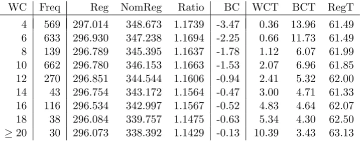
3.4.2 Results and Discussion

We present key values for worst-case inverse problems in Table 4. We categorized in-stances according to the objective value ”WC” of the worst-case problem. The smallest observed objective value was 4, and the largest was 28 (the value 2 could not be achieved, as we required the difference between regret values to be at least 1).

Column ”Freq” denotes how often an objective value was observed over the 2,500 instances. Columns ”Reg” and ”NomReg” show the average optimal regret, and the average regret of the nominal solution within each instance class, respectively. In column ”Ratio”, the ratio between these two values is given. Column ”BC” shows the average best-case inverse value for problems within each class. The BC values are given as the negative difference to the maximum BC value, which is 9000 (i.e., smaller BC values mean that the largest possible interval uncertainty for which the nominal solution is also the optimal solution for the regret problem is smaller). ”WCT” and ”BCT” show the average time to solve the worst-case and the best-case inverse problems in seconds, respectively. ”RegT” is the average time to solve the 500 min-max regret problems we generated per instance and is also given in seconds.

WC Freq Reg NomReg Ratio BC WCT BCT RegT

4 569 297.014 348.673 1.1739 -3.47 0.36 13.96 61.49 6 633 296.930 347.238 1.1694 -2.25 0.66 11.73 61.49 8 139 296.789 345.395 1.1637 -1.78 1.12 6.07 61.99 10 662 296.780 346.153 1.1663 -1.53 2.07 6.96 61.85 12 270 296.851 344.544 1.1606 -0.94 2.41 5.32 62.00 14 43 296.754 343.172 1.1564 -0.47 3.00 4.71 61.33 16 116 296.534 342.997 1.1567 -0.52 4.83 4.64 62.07 18 38 296.084 339.757 1.1475 -0.63 5.34 4.30 62.50

≥20 30 296.073 338.392 1.1429 -0.13 10.39 3.43 63.13 Table 4: Statistics for worst-case inverse problems.

solution improves for larger values of WC. As the nominal solution is sometimes used as the baseline heuristic for solution algorithms (see, e.g., [CG15]), this may lead to structural insight on the performance of such algorithms for different instance classes.

The computation time for WC increases with the resulting objective value, while computation times for BC decreases for the respective instance classes. WC and BC values are connected, with instances having small WC values also tending to have large BC values. That is, if only little uncertainty is required to disturb the nominal solution, then the largest possible uncertainty set for which it is optimal also tends to be smaller. Our results do not show a significant increase in computation time for RegT, depending on WC.

Summarizing, we find that the WC value is able to categorize instances according to the relative performance of the nominal solution. While the ratio of NomReg and Reg is easier to compute than WC, if offers structural insight on why these instances behave differently, and can be used to structure benchmark sets as an example application.

4 Conclusion and Further Research

In classic robust optimization problems, one aims at finding a solution that performs well for a given uncertainty set of possible parameter outcomes. In this paper, we considered a more general problem where we assume only the shape of the uncertainty set to be given, but not its actual size.

The resulting variable-sized min-max robust optimization problem is analyzed for different uncertainty sets, and results are applied to the shortest path problem. In a brief case study, we demonstrated the value of alternative solutions to the decision maker, which can be found in little computation time.

As a special case of variable-sized uncertainty, we considered inverse problems with min-max regret objective. To solve such problems, mixed-integer programming formu-lations were derived. Inverse robust optimization can also be applied to give structural insight to robust optimization instances, which was demonstrated with experimental data.

Our research is the first of its kind, with possible applications in decision support, sensitivity analysis, and benchmarking.

References

[ABP09] B. Alizadeh, R. E. Burkard, and U. Pferschy. Inverse 1-center location problems with edge length augmentation on trees. Computing, 86(4):331– 343, 2009.

[ABV09] H. Aissi, C. Bazgan, and D. Vanderpooten. Min–max and min–max re-gret versions of combinatorial optimization problems: A survey. European Journal of Operational Research, 197(2):427 – 438, 2009.

[AO01] R. K. Ahuja and J. B. Orlin. Inverse optimization. Operations Research, 49(5):771–783, 2001.

[BB09] D. Bertsimas and D. B. Brown. Constructing uncertainty sets for robust linear optimization. Operations Research, 57(6):1483–1495, 2009.

[BBC11] D. Bertsimas, D. Brown, and C. Caramanis. Theory and applications of robust optimization. SIAM Review, 53(3):464–501, 2011.

[BG16] H. Bar-Gera. Transportation network test problems, http://www.bgu.ac.il/∼bargera/tntp/, accessed 06/2016.

[BPS04] D. Bertsimas, D. Pachamanova, and M. Sim. Robust linear optimization under general norms. Operations Research Letters, 32(6):510 – 516, 2004.

[BS04] D. Bertsimas and M. Sim. The price of robustness. Operations Research, 52(1):35–53, 2004.

[BTdHV15] A. Ben-Tal, D. den Hertog, and J. Vial. Deriving robust counterparts of nonlinear uncertain inequalities. Mathematical Programming, 149(1):265– 299, 2015.

[BTGN09] A. Ben-Tal, L. El Ghaoui, and A. Nemirovski.Robust Optimization. Prince-ton University Press, PrincePrince-ton and Oxford, 2009.

[Car83] P. J. Carstensen.The complexity of some problems in parametric linear and combinatorial programming. University of Michigan, 1983.

[CG15] A. Chassein and M. Goerigk. A new bound for the midpoint solution in minmax regret optimization with an application to the robust shortest path problem. European Journal of Operational Research, 244(3):739–747, 2015.

[CG16a] A. Chassein and M. Goerigk. Compromise solutions for robust combi-natorial optimization with variable-sized uncertainty. Technical report, arXiv:1610.05127, 2016.

[CG17] A. Chassein and M. Goerigk. Minmax regret combinatorial optimization problems with ellipsoidal uncertainty sets.European Journal of Operational Research, 258(1):58–69, 2017.

[CN03] E. Carrizosa and S. Nickel. Robust facility location. Mathematical Methods of Operations Research, 58(2):331–349, 2003.

[GKR12] J. Gorski, K. Klamroth, and S. Ruzika. Generalized multiple objective bottleneck problems. Operations Research Letters, 40(4):276–281, 2012.

[GS16] M. Goerigk and A. Sch¨obel. Algorithm engineering in robust optimization. In L. Kliemann and P. Sanders, editors, Algorithm Engineering: Selected Results and Surveys, volume 9220, pages 245–279. Springer, 2016.

[GYd15] B. L. Gorissen, ˙I. Yanıko˘glu, and D. den Hertog. A practical guide to robust optimization. Omega, 53:124–137, 2015.

[Heu04] C. Heuberger. Inverse combinatorial optimization: A survey on problems, methods, and results.Journal of Combinatorial Optimization, 8(3):329–361, 2004.

[IT13] D. A. Iancu and N. Trichakis. Pareto efficiency in robust optimization. Management Science, 60(1):130–147, 2013.

[JJNS16] P. Jaillet, S. D. Jena, T. S. Ng, and M. Sim. Satisficing awakens: Mod-els to mitigate uncertainty. Technical report, Massachusetts Institute of Technology, 2016.

[JMSSM05] O. Jahn, R. H. M¨ohring, A. S. Schulz, and N. E. Stier-Moses. System-optimal routing of traffic flows with user constraints in networks with con-gestion. Operations research, 53(4):600–616, 2005.

[KY97] P. Kouvelis and G. Yu. Robust Discrete Optimization and Its Applications. Kluwer Academic Publishers, 1997.

[Mor86] H. I. Mordechai. The shortest path problem with two objective functions. European Journal of Operational Research, 25(2):281–291, 1986.

[NC15] K. T. Nguyen and A. Chassein. The inverse convex ordered 1-median prob-lem on trees under chebyshev norm and hamming distance.European Jour-nal of OperatioJour-nal Research, 247(3):774 – 781, 2015.

[Pos13] M. Poss. Robust combinatorial optimization with variable budgeted uncer-tainty. 4OR, 11(1):75–92, 2013.

[RCH+_{16] B. Rostami, A. Chassein, M. Hopf, D. Frey, C. Buchheim, F.}