Modeling and Numerical Simulation of Ammonia Synthesis Reactors Using Compositional Approach

ISSN Online: 2160-0406 ISSN Print: 2160-0392

DOI: 10.4236/aces.2018.83009 Jul. 23, 2018 124 Advances in Chemical Engineering and Science

Modeling and Numerical Simulation of

Ammonia Synthesis Reactors Using

Compositional Approach

Diogo Silva Sanches Jorqueira

, Antonio Marinho Barbosa Neto

,

Maria Teresa Moreira Rodrigues

1_{Department of Chemical Systems Engineering, Campinas University, Campinas, Brazil} 2_{Simworx, Engineering, Research & Development, Campinas, Brazil}

Abstract

Ammonia synthesis reactors operate in conditions of high pressure and high temperature. Consequently, the flow inside these reactors always presents in-teraction between components in the feed mixture. A modeling accounts these interactions with pressure, temperature and the molar fraction is essen-tial to converter simulation more realistic. The compositional approach based on cubic equations of state provides the influences of the component of a gas mixture using mixing rules and binary interaction parameters. This multi-component description makes the model more robust and reliable for proper-ties mixture prediction. In this work, two models of ammonia synthesis reac-tors were simulated: adiabatic and autothermal. The fitted expression of Singh and Saraf was used. The adiabatic reactor model presented a maximum rela-tive error of 1.6% in temperature and 11.4% in conversion while the auto-thermal reactor model presents a maximum error of 2.7% in temperature, when compared to plant data. Furthermore, a sensitivity analysis in input va-riables of both converter models was performed to predict operational limits and performance of the Models for Ammonia Reactor Simulation (MARS).

Keywords

Cubic Equation of State, Adiabatic Converter, Autothermal Converter, Temkin-Pyzhev Expression

1

.

Introduction

In ammonia synthesis, fixed bed reactors are always used. Only one reaction

oc-curs in the gas phase using iron catalyst particles [1] [2], as described in

Equa-tion (1).

How to cite this paper: Jorqueira, D.S.S., Neto, A.M.B. and Rodrigues, M.T.M. (2018) Modeling and Numerical Simulation of Ammonia Synthesis Reactors Using Com- positional Approach. Advances in Chemical Engineering and Science, 8, 124-143.

https://doi.org/10.4236/aces.2018.83009

Received: June 18, 2018 Accepted: July 20, 2018 Published: July 23, 2018

Copyright © 2018 by authors and Scientific Research Publishing Inc. This work is licensed under the Creative Commons Attribution International License (CC BY 4.0).

http://creativecommons.org/licenses/by/4.0/

D. S. S. Jorqueira et al.

DOI: 10.4236/aces.2018.83009 125 Advances in Chemical Engineering and Science

2 2 3 3

N 3H 2NH , Δ o 45.94 kJ mol of NH

r

H

+ ↔ = − ₍₁₎

The reaction is exothermic in pressures from 150 to 300 atm, due to the de-crease in mole numbers. Moreover, the temperature range is 600 to 800 K. After all, even with an exothermic reaction, the reaction rate in converters must be high. The High Pressure and High Temperature (HPHT) conditions in gas phase make properties in reactive fluid temperature vary too much along the conver-ter. Some examples are density, fugacity, chemical activity and heat capacity.

The mathematical modeling of ammonia converters uses experimental rate

expressions. They generally contain partial pressures [1] or chemical activities

[2] in formulation. One of the first models was presented by the authors Emmett

and Kummer [3]. They used Temkin and Pyzhev expression [1] to obtain

expe-rimental and predicted data. Moreover, they proposed the formulation of a reac-tion rate using fugacity and not partial pressures.

After a few years, many researchers continued to use Temkin and Pyzhev rate

in their calculations [4] [5] [6] [7]. However, in 1964, Nielsen and collaborators

proposed modifications in reaction rate [8]. They verified that chemical activities could be included in the rate model.

Dyson and Simon [2] also used chemical activities in their work. They also

proposed a kinetic correction factor to a heterogeneous reaction. Many studies continued to use Dyson and Simon expression, with small modifications. Many presented good validation with plant data and were focused on optimization analysis [9]-[15].

However, in previous publications, the fugacity coefficients were derived from a correlation that they varied with temperature and pressure, but not

composi-tion [9]-[15]. The implications are that the chemical activity does not change

with molar and mass fraction variations inside the reactor. Moreover, the mass, energy and momentum balances provided remarkable composition variations, even with only one reaction. This effect is more pronounced when fluid presents differences in molar weight (which is the case of ammonia production).

Therefore, a more sophisticated model can be used to provide a multicom- ponent description. This method is the principle of the compositional approach: the reactant fluid present changes of properties influenced not only by pressure and temperature but also by composition and intermolecular forces. The last and more important part is computed due to mixing rules in cubic EoS calculations. Furthermore, two facts reinforce the use of a compositional approach in ammo-nia synthesis: 1) the molecules in the gas phase are smaller and 2) the high- pressure deviates gas from ideal treatment, approximating gas molecules.

As most of substances are non-polar (except for NH3) and gases are at HPHT

conditions, the Peng-Robinson (PR) and Soave-Redlich-Kwong (SRK) cubic EoS are chosen to model the system. Therefore, the EoS approach will replace the previous activities used in reaction rate. As discussed above, these models present a more reliable theory and a molecular formulation.

DOI: 10.4236/aces.2018.83009 126 Advances in Chemical Engineering and Science

with plant data (adiabatic and autothermal); use a fitted reaction rate using a compositional approach; solve mass, energy and momentum balances in PFR model in steady-state and present a study of parametric sensitivity in input va-riables of ammonia converters.

2

.

Mathematical Background

2.1

.

Thermodynamic Modeling

The SRK [16] and PR [17] cubic EoS are the two most widely used cubic

equa-tions in the process industry. According to Ahmed [18], the general form of

two-parameter cubic EoS is shown at Equation (2).

(

)(

)

RT a

p

v b v δb v δ b

= −

− + + (2)

For the results of this work, only PR-EoS was used, with the parameters

0.5 1 1 2

δ

2 1 2

δ

( )

ap A

RT

= ₍₃₎

bp b

RT

= ₍₄₎

pv Z

RT

= ₍₅₎

and substituting into Equation (2), as described at Barbosa Neto [19], the

impli-cit form of the cubic EoS, in the compressibility factor Z, is obtained:

(

)

(

) (

)

(

)

3 2 2

1 2 1 2 1 2

2 1 2

1 1 1

1 0

Z B Z A B B B Z

AB B B

δ δ δ δ δ δ

δ δ

 

+_ + − − _ +_ + − + + _

 

−_ + + _= (6)

The van der Waals one-fluid mixing rules are used for the energy A, and for

the volume B, parameters of the EoS, are expressed by Equations (7) and (8),

re-spectively.

1 1

nc nc i j ij i j

A y y A

= =

=

∑∑

1

nc i i i

B y B

=

=

∑

The parameter Aij, in the Equation (7), is calculated from Equation (9).

(

)

ij i j ij

A = A A −k (9)

The terms Ai and Bi are defined by Equations (10) and (11), respectively. The

factor m(ωi) is given in the literature [17]. Values of Ωa and Ωb changes with

EOS.

( )

(

)

2 1 1

ri

i a i ri

ri

p

A m T

T ω

 _{  }

= Ω _{  } + − _

  (10)

ri i b ri p B T   = Ω  

D. S. S. Jorqueira et al.

DOI: 10.4236/aces.2018.83009 127 Advances in Chemical Engineering and Science

The expression shown at Equation (12) for fugacity coefficients is obtained.

( ) (

)

(

)

2

2

ln 1 i ln i i ln

i Z B_B Z B A_{B A} B_{B Z}Z B_B

ψ δ ϕ δ  +       = − _{ }− − −_{ } − _{  } ∆ +  

      (12)

With ∆ = −δ δ1 2 and

1

nc

i i j j

i A y

ψ

=

=

∑

The fugacity and activity are also important for reaction rate used. They are given in Equations (14) and (15).

i i i

f =ϕy P ₍₁₄₎

i i i

i

ref ref

y P f a

P P

ϕ

= = (15)

Other important properties are the heat capacities, which are given in Equa-tions (16) and (17). More details are found in Tosun [20].

ig res

p p p

C =C +C ₍₁₆₎

ig res

v v v

C C= +C ₍₁₇₎

2.2

.

Rate Expression

The rate used in ammonia reactors of this research was made by Singh and Saraf

[9], as given in Equation (18). We compute the chemical activities predicted by a

suited thermodynamic model. The previous works presented fugacity coeffi-cients given correlations [2].

3 2 3 2 3 2 1 2 3 NH H 10 2

NH N 2 3

NH H

163422

4.11 10 exp eq

a a

r K a

RT a a

α −α

 _{   } 

−

 _{  }

= × _{ } _ _ −_ _

 

 _{     } (18)

The rate given in Equation (18) is pseudo-homogeneous. Nielsen and colla-borators provided a suitable range for ammonia rate expressions: 640 to 770 K

and 150 to 310 atm [8]. Therefore, it was corrected by an effectiveness factor η

for a heterogeneous reactor, as shown in Equation (19) and Table 1.

2 2 2

2 3 3

0 1 2 N 3 4 N 5 6 N

b bT b x b T b x b T b x

η

To summarize this section, the equilibrium constant (Keq) in Equation (19) is

found in correlation given by Gillespie and Beattie [21].

Table 1. Coefficients for Equation (19) [2].

P (atm) b0 b1 b2 b3 b4 b5 b6

150 −17.539 0.0769 6.901 −1.083 × 10−4 _{−26.425 4.928 × 10}−8 _38.937

225 −8.213 0.0377 6.190 −5.355 × 10−5 _{−20.869 2.379 × 10}−8 _27.880

DOI: 10.4236/aces.2018.83009 128 Advances in Chemical Engineering and Science

2.3

.

Mass, Momentum and Energy Balances (Adiabatic Reactors)

In the adiabatic operation of ammonia reactors, the volume of control increases its temperature using only the heat of reaction. However, this operation is not possible in one converter. The reactor volume must be separated into several reactors, as given in Figure 1.

The mass balance in one reactor is expressed only regarding nitrogen conver-sion (Equations (20) and (21)) because only one reaction takes place in converter

[2]. The only difference between the following relations is the area of reactor.

Therefore, the coordinates can be done in length L or volume V.

3 2 2 NH N 0 N d d 2 Ar x L F η

= ₍₂₀₎

3 2 2 NH N 0 N d d 2 r x V F η

= ₍₂₁₎

Equations (22) and (23) express the energy balances. As the reactor is at high

pressure, the estimation of Cp is essential. Moreover, the heat of reaction is

computed according to correlation [21].

(

)

η

(

)

Besides, as reactor contains catalyst particles, there is a pressure loss along the

converter. It is estimated using the Ergun Equation [22], as expressed in

Equa-tion (24). However, this relaEqua-tion is only for dP computations in length L. For dV computations, the pressure loss dP/dV is set to zero [9].

(

)

(

)

3 2 3

150 1 1.75 1

d

d p p

u u

P

L d d

ε µ ε ρ

ε ε

− −

= − ₍₂₄₎

2.4

.

Mass, Momentum and Energy Balances (Autothermal

Reactors)

The autothermal reactor uses the energy released by a reaction to heat the reac-tant gas. It operates with countercurrent flow, and it is divided into several tubes, as given in Figure 2. The catalyst is inside the tubes, while the cooling gas increases its temperature along the converter.

D. S. S. Jorqueira et al.

DOI: 10.4236/aces.2018.83009 129 Advances in Chemical Engineering and Science

Figure 2. Scheme of an autothermal reactor [23].

The mass balance and pressure loss in the autothermal converter do not change compared to the adiabatic model. The difference is in the temperature: now we have the reactant gas (that increases its temperature by the reaction and is cooling by cooling gas) and the cooling gas (that always increases its tempera-ture). The energy balances are given in Equations (25) and (26) (for length vari-ations) and Equations (27) and (28) (for volume varivari-ations). The minus sign in Equations (26) and (28) is related to countercurrent operation.

(

)

(

)

3

NH

d

d _{mix mix}

g r

p p

UA T T

Ar H

T

L mC mC

η −∆ ′ −

= −

(25)

(

)

d

d _mix

g g

p

UA T T T

L mC

′ − = −

(26)

(

)

(

)

3

NH

d

d _{mix mix}

g r

p p

Ua T T

r H

T

V mC mC

η −∆ ′ −

= −

(27)

(

)

d

d _mix

g g

p

Ua T T T

V mC

′ − = −

(28)

3

.

Methodology

3.1

.

Solution of ODEs System

DOI: 10.4236/aces.2018.83009 130 Advances in Chemical Engineering and Science

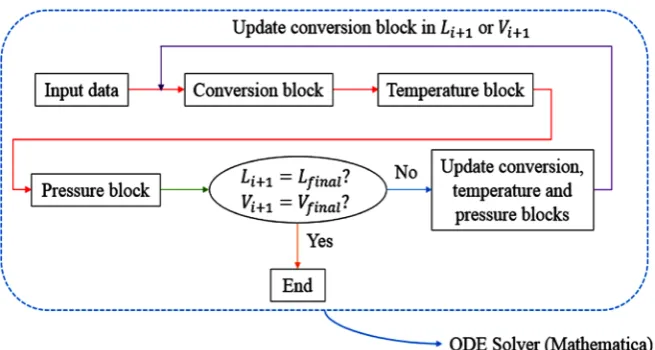
Another challenge is the interdependence of variables in differential equa-tions. Therefore, the code was made using a modular structure in Wolfram Ma-thematica® Programming Language. Moreover, our algorithm is called MARS (Models for Ammonia Reactor Simulation).

The variables of interest in both models are the outlet temperature, pressure, and composition. The thermodynamic module computes the thermodynamic and transport properties; the kinetic module calculates the reaction rate and another module joins all the previous in a numerical method to solve the bal-ances. As the problem is solved in one dimension, the stopping-criteria is the end of the reactor, as expressed in Figure 3.

3.2

.

Variation of

α

in Reaction Rate

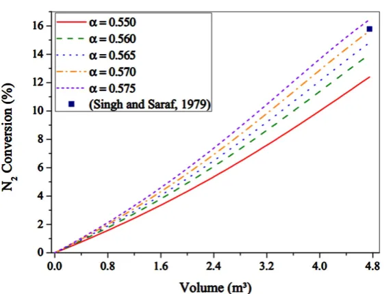
As discussed before, the chemical activities originally are computed using a cor-relation—Singh and Saraf Rate (Equation (18)). However, when using the mul-ticomponent approach, it is expected that chemical activity decreases, due to compositional interactions. Therefore, the reaction rate computed also decreases its value. So, the kinetic factor α is fitted in MARS. The fit is made according to an adiabatic reactor in the literature [9]. Only the first bed is calculated in

tem-perature and conversion. Table 2 shows the parameters for this reactor.

Figure 4 presents the N2 conversion variation in an adiabatic converter with α

alterations.

Figure 3. Flowchart for calculation of reactor.

Table 2. Input parameters and plant data for the 1st reactor [9].

Parameter Value Parameter Value Parameter Value Exp. Data Value

2 N

y 0.2219 yNH3 0.0546 Tin (K) 658.15 Tout1 (K) 780.15

2 H

y 0.6703 yAr 0.0256 Pin (atm) 226 xN out12 (%) 15.78

3 NH

D. S. S. Jorqueira et al.

DOI: 10.4236/aces.2018.83009 131 Advances in Chemical Engineering and Science

Figure 4. Conversion profile in first bed using α variations at MARS (EoS approach).

The outlet conversion increases when α rises because the reaction rate is

higher. Moreover, at α = 0.570, the model does well in predicting the outlet

con-version. Therefore, the original value of α = 0.550 in Singh and Saraf rate [9]

should be replaced by α = 0.570 when using the compositional approach from

now on. The conversion was chosen because it is the variables which have more effect on output composition and its error is more significant than temperature.

4

.

Results and Discussions

For validations in adiabatic and autothermal models, the relative error was cal-culated as expressed in Equation (29). In the case of multiple reactors, the max-imum relative error will be taken.

data data

error

data

plant simulation

rel 100

plant

−

= ₍₂₉₎

Even with a suitable numerical method and a robust code, validations of

reac-tors models are necessary. The RKF method and α = 0.570 are selected for Singh

and Saraf modified rate. Furthermore, calculates an adiabatic reactor containing three fixed beds in series and an autothermal converter. Both models are reliable compared to plant data.

4.1

.

Model Validation

4.1.1. Adiabatic Reactor

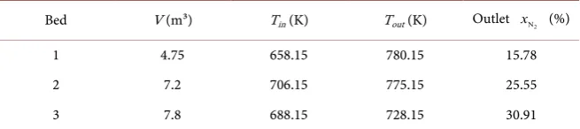
In adiabatic case, we have three reactors in series. The first bed is computed in a variation of α. Therefore, all inlets parameters remain the same. The only addi-tional information for simulation is the inlet temperature of the second and third reactors and their respective volume, as given in Table 3.

Figure 5 shows the temperature profile obtained. In this, the highest errors in

DOI: 10.4236/aces.2018.83009 132 Advances in Chemical Engineering and Science

Figure 5. Plant data and MARS EoS model temperature profile (adiabatic reactor).

Table 3. Plant data for three adiabatic beds in series [9].

Bed V (m³) Tin (K) Tout (K) Outlet xN2 (%)

1 4.75 658.15 780.15 15.78

2 7.2 706.15 775.15 25.55

3 7.8 688.15 728.15 30.91

place where the rate has its highest values. Therefore, it can provide more errors compared to the others. However, in the second and third converters, the simu-lated temperature gives good results compared to plant data. In all simulations of the adiabatic arrangement, 74 iterations are required with RKF. It is a good

result compared if the 4th _{Order Runge-Kutta with fixed step size was used (with}

50 iterations at each reactor, for example).

In addition, Table 4 presents the relative errors of temperature. It proves a

good comparison between MARS and plant data (Singh and Saraf, 1979) [9].

The maximum error of temperature reached by other authors was less than 6% (Singh and Saraf, 1979) [9].

Even with good results in temperature predictions, the conversion is another crucial variable. The composition of the reactor depends on conversion, after all.

Furthermore, it is more sensitive to variations than temperature. Figure 6 shows

the conversion profile computed by MARS.

In Figure 6, the highest error in conversion occurred in the third reactor. The

first and second converters presented a good agreement with plant data. The main error in the third reactor is the previous errors inherited by the first and second reactors (the error was propagated). Moreover, the final converter is where the reaction rate presents the smallest value. The relative errors in

conver-sion are summarized in Table 5. To summarize, even with the difference in

D. S. S. Jorqueira et al.

DOI: 10.4236/aces.2018.83009 133 Advances in Chemical Engineering and Science

Figure 6. Plant data and MARS EoS model conversion profile (adiabatic reactor).

Table 4. Comparison between outlet temperature in plant data and the MARS model.

Bed ToutPlant (K) ToutMARS (K) Rel Error (%)

1 780.15 768.04 1.55

2 775.15 773.14 0.26

3 728.15 730.46 0.32

Table 5. Comparison between outlet conversion in plant data and the MARS model.

Bed xN out Plant2 (%) xN out MARS2 (%) Rel Error (%)

1 15.78 15.64 0.88

2 25.55 26.64 4.27

3 30.91 34.42 11.36

simulation, because the temperature is usually the control variable in ammonia reactors. Errors in literature reached less than 0.5% [9].

4.1.2. Autothermal Reactor

The autothermal converter has the reactor parameters given in Table 6. In this

type of converter, the temperature is measured in several points of the reactor.

In Figure 7, differences are noted between simulation and plant data for

reac-tant gas temperature inside reactor. First, only at the end of the autothermal reactor are the differences significant. These occur due to a change of dynamics in the ODE system.

However, the maximum temperature point is well predicted, which reinforces the method’s effectiveness. The maximum relative error was 2.7% in the end of reactor, due to high nonlinearity of equations.

DOI: 10.4236/aces.2018.83009 134 Advances in Chemical Engineering and Science

Figure 7. Comparison between the MARS EoS model and plant data

(auto-thermal reactor).

Table 6. Input parameters for autothermal reactor [9].

Parameter Value Parameter Value Parameter Value

2 N

y 0.2190 yAr 0.0360 V (m3) 4.07

2 H

y _0.6500 m (kg/s) 6.038 a' (m2_/m3_{) 10.29}

3 NH

y _0.0520 Tin (K) 694.15 U (W/m2∙K) 465.2

4 CH

y _0.0430 Pin (atm) 279

Table 7. Relative errors in reactant gas temperature in autothermal reactor [9].

V (m3_{) T}

plant (K) Rel. Error (%) V (m3) Tplant (K) Rel. Error (%)

0 694.15 0.00 2.21 781.15 0.01

0.17 716.15 1.47 2.54 771.15 0.17

0.51 759.15 1.78 2.88 756.15 1.27

0.85 789.15 1.05 3.22 748.15 1.28

1.19 799.15 0.07 3.56 733.15 1.68

1.53 796.15 0.46 3.90 719.15 1.84

1.87 787.15 0.56 4.07 711.15 2.66

proves the reliability of the MARS model for the autothermal reactor. Other au-thors reached 3.2% of maximum relative difference in temperature, which was an acceptable value [9].

4.2

.

Sensitivity Analysis

D. S. S. Jorqueira et al.

DOI: 10.4236/aces.2018.83009 135 Advances in Chemical Engineering and Science

adiabatic model, the analysis is realized in three reactors in series. The inlet temperature was varied. Then, the effects on temperature, conversion and effec-tiveness factor profiles were detected in each case. While, in the autothermal model, the heat exchange coefficient was varied, with the same detections on output of reactor. The variations were computed in length L.

4.2.1. Adiabatic Reactor

Figure 8 presents the adiabatic reactors flowchart and dimensions. In all the

analysis, the reactor consists of 3 beds, with indirect cooling. The values of vo-lume and length were estimated using literature [9] [12].

In adiabatic operation, only the inlet temperature of the 1st _{reactor is varied.}

The temperatures Tin2 and Tin3 maintain the same values (as given in Table 8).

Moreover, the RKF method with variable step size is used for numerical simula-tion.

The inlet temperature effect along converter temperature is given in Figure 9.

Analyzing the Figure 9, we can note that the lowest inlet temperature (Tin =

643.15 K) gave the highest profiles along second and third reactors. After all, smaller temperatures provide smaller rates, which give minor conversions.

Therefore, after first reactor, more N2 can be converted, giving a more

accen-tuated profile (Tin = 643.15 K).

On the other hand, high inlet temperatures present high reaction rates,

con-verting more N2 in the first bed. However, it becomes more difficult to react in

the second and third converters. Therefore, the temperature rise is not so signif-icant as in smaller Tin values, even with high rates. In the three cases, the number of iterations during the converging process is similar.

Figure 8. Flowchart for adiabatic beds parametric sensitivity.

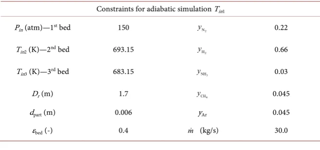
Table 8. Parameters for inlet temperature variation in adiabatic model (643.15 K, 663.15

K and 683.15 K).

Constraints for adiabatic simulation Tin1

Pin (atm)—1st bed 150 yN2 0.22

Tin2 (K)—2nd bed 693.15 yH2 0.66

Tin3 (K)—3rd bed 683.15 yNH3 0.03

Dr (m) 1.7 yCH4 0.045

dpart (m) 0.006 yAr 0.045

DOI: 10.4236/aces.2018.83009 136 Advances in Chemical Engineering and Science

Figure 9. Temperature profiles in beds (Tin = 643.15 K, 663.15 K and 683.15 K).

Another essential measure inside our reactor is the composition. As there is only one reaction, the conversion profile gives the other molar fractions

indi-rectly. For the inlet temperature variation case, Figure 10 shows the conversion

profile.

In Figure 10, it is noted that larger inlet temperatures give higher N2

conver-sions. However, a high Tin does not guarantee to elevate conversions, because the reaction is exothermic. After all, the reaction is reversible, and high temper-atures provide low equilibrium conversion. Moreover, the highest rise in con-versions occurs in the first bed. It can be seen that the growth of conversion be-tween interval of 683.15 K and 663.15 K is smaller than 663.15 K and 643.15 K. Therefore, there is a limit to the Tin value.

Figure 11 shows the effectiveness factor profiles. As inlet temperature

in-creases, η factor also increases. This occurs due to a higher reaction rate. More-over, the first reactor presents the smaller values of η. After all, the overall con-version is lower in first reactor.

4.2.2. Autothermal Reactor

Figure 12 presents the autothermal reactor flowchart and dimensions.

The parameters for simulation are given in Table 9.

Figure 13 presents the reactant gas temperatures profiles. In this, we note that

the length in the reactor which presents the largest temperature does not change.

However, the maximum temperature value for U = 450 W/m2_{∙K is 753 K, while}

for U = 650 W/m2_{∙K, is 739 K. Moreover, another important value is the final}

value of temperature for the reactant gas at the end of the reactor. For U = 450

W/m2_{∙K, the final T value is 724 K and U = 650 W/m}2_{∙K is 687 K. It takes place}

D. S. S. Jorqueira et al.

DOI: 10.4236/aces.2018.83009 137 Advances in Chemical Engineering and Science

Figure 10. Conversion profiles in beds (Tin = 643.15 K, 663.15 K and 683.15 K).

Figure 11. Effectiveness factor profiles in beds (Tin = 643.15 K, 663.15 K and 683.15 K).

Table 9. Parameters for inlet temperature variation in autothermal model (450, 650 and

850 W/m2_∙K).

Constraints for countercurrent simulation

2 N

y 0.22 nt 250

2 H

y 0.66 Dr (m) 1.5

3 NH

y 0.03 Lr (m) 2.5

4 CH

y 0.045 a' (m2_{/m) 11.78}

yAr 0.045 m (kg/s) 6.0

DOI: 10.4236/aces.2018.83009 138 Advances in Chemical Engineering and Science

Figure 14 presents the conversion profile. When U increases, the final

con-version also increases. It occurs because more energy is removed by the reaction,

decreasing the speed of the reverse reaction. However, U cannot be raised too

much, otherwise the rate would be very low.

The effectiveness factor η profiles are given in Figure 15. As U increases, the

temperature decreases in the reactor, raising equilibrium conversion and η values.

However, in U = 850 W/m2_{∙K, there are errors computing η (higher than 1).}

Figure 12. Adiabatic reactor flowchart and dimensions.

Figure 13. Reactant gas temperature profiles in autothermal reactor (U = 450, 650

and 850 W/m2_∙K).

D. S. S. Jorqueira et al.

DOI: 10.4236/aces.2018.83009 139 Advances in Chemical Engineering and Science

Figure 15. Effectiveness factor profiles in autothermal reactor (U = 450, 650

and 850 W/m2_∙K).

5

.

Conclusions

The compositional modeling using PR cubic EoS was essential to calculate the properties in reactive streams at HPHT conditions during the ammonia synthe-sis reactors simulation. The adiabatic reactor model presented a maximum rela-tive error of 1.6% in temperature and 11.4% in conversion when compared to plant data. In sensitivity study, a value of Tin = 683.15 K gave the highest conver-sion of 25.16%. The autothermal reactor model presented a maximum error of 2.7% in temperature when compared to experimental points. In parametrical

sensitivity, the highest conversion of 37.22% was provided by a value of U = 850

W/m2_{∙K. Therefore, both models proved reliable in simulating ammonia}

reac-tors for the set of data used.

Another improvement of the ammonia synthesis reactor models can be achieved using intraparticle diffusional approach. It computes the effectiveness factor without using an experimental correlation.

Acknowledgements

The authors acknowledge CNPq (Process Number 131744/2016-0) and Unicamp for providing financial support.

References

[1] Temkin, M. and Pyzhev, V. (1939) Kinetics of the Synthesis of Ammonia on Pro-moted Iron Catalysts. Journal of Physical Chemistry,13, 851.

[2] Dyson, D.C. and Simon, J.C. (1968) A Kinetic Expression with Diffusion Correction for Ammonia Synthesis on Industrial Catalyst. Industrial and Engineering Chemistry Fundamentals, 7, 605-610.https://doi.org/10.1021/i160028a013

[3] Emmett, P.H. and Kummer, J.T. (1943) Kinetics of Ammonia Synthesis. Industrial and Engineering Chemistry, 35, 677-683.https://doi.org/10.1021/ie50402a012

DOI: 10.4236/aces.2018.83009 140 Advances in Chemical Engineering and Science Synthesis in Large-Scale Reactors. Chemical Engineering Science, 1, 145-154.

https://doi.org/10.1016/0009-2509(52)87011-3

[5] Baddour, R.F., Brian, P.L.T., Logeais, B.A. and Eymery, J.P. (1965) Steady-State Si-mulation of an Ammonia Synthesis Converter. Chemical Engineering Science, 20, 281-292.https://doi.org/10.1016/0009-2509(65)85017-5

[6] Brian, P.L.T., Baddour, R.F. and Eymery, J.P. (1965) Transient Behaviour of an Ammonia Synthesis Reactor. Chemical Engineering Science, 20, 297-310.

https://doi.org/10.1016/0009-2509(65)85019-9

[7] Murase, A., Roberts, H.L. and Converse, A.O. (1970) Optimal Thermal Design of an Autothermal Ammonia Synthesis Reactor. Industrial & Engineering Chemistry Process Design and Development, 9, 503-513.https://doi.org/10.1021/i260036a003

[8] Nielsen, A., Kjaer, J. and Hansen, B. (1964) Rate Equation and Mechanism of Am-monia Synthesis at Industrial Conditions. Journal of Catalysis, 3, 68-79.

https://doi.org/10.1016/0021-9517(64)90094-6

[9] Singh, C.P.P. and Saraf, D.N. (1979) Simulation of Ammonia Synthesis Reactors.

Industrial & Engineering Chemistry Process Design and Development, 18, 364-370.

https://doi.org/10.1021/i260071a002

[10] Elnashaie, S.S., Abashar, M.E. and Al-Ubaid, A.S. (1988) Simulation and Optimi-zation of an Industrial Ammonia Reactor. Industrial and Engineering Chemistry Re-search, 27, 2015-2022.https://doi.org/10.1021/ie00083a010

[11] Dashti, A., Khorsand, K., Marvast, M.A. and Kakavand, M. (2006) Modeling and Simulation of Ammonia Synthesis Reactor. Petroleum & Coal, 48, 15-23.

[12] Azarhoosh, M.J., Farivar, F. and Ale Ebrahim, H. (2014) Simulation and Optimization of a Horizontal Ammonia Synthesis Reactor Using Genetic Algorithm. RSC Ad-vances, 4, 13419-13429.https://doi.org/10.1039/C3RA45410J

[13] Farivar, F. and Ale Ebrahim, H. (2014) Modeling, Simulation, and Configuration Improvement of Horizontal Ammonia Synthesis Reactor. Chemical Product and Process Modeling, 9, 89-95.https://doi.org/10.1515/cppm-2013-0037

[14] Akpa, J.G. and Raphael, N.R. (2014) Optimization of an Ammonia Synthesis Converter. World Journal of Engineering and Technology, 2, 305-313.

[15] Khademi, M.H. and Sabbaghi, R.S. (2017) Comparison between Three Types of Ammonia Synthesis Reactor Configurations in Terms of Cooling Methods. Chemical Engineering Research and Design, 128, 306-317.

https://doi.org/10.1016/j.cherd.2017.10.021

[16] Soave, G. (1972) Equilibrium Constants from a Modified Redlich-Kwong Equation of State. Chemical Engineering Science, 27, 1197-1203.

https://doi.org/10.1016/0009-2509(72)80096-4

[17] Peng, D.Y. and Robinson, D.B. (1976) A New Two-Constant Equation of State. In-dustrial & Eng. Chemistry Fundamentals, 15, 59-64.

https://doi.org/10.1021/i160057a011

[18] Ahmed, T. (2016) Equations of State and PVT Analysis: Applications for Improved Reservoir Modeling. 2nd Edition, Elsevier, New York.

[19] Barbosa Neto, A.M. (2015) Desenvolvimento de um Simulador PVT Composicional para Fluidos de Petróleo. Masters Dissertation, University of Campinas, Campinas. [20] Tosun, I. (2013) The Thermodynamics of Phase and Reaction Equilibria. Elsevier,

New York.

Ap-D. S. S. Jorqueira et al.

DOI: 10.4236/aces.2018.83009 141 Advances in Chemical Engineering and Science

plied to Ammonia Synthesis. The Energy and Entropy Constants for Ammonia.

Physical Review, 36, 1008-1013.https://doi.org/10.1103/PhysRev.36.1008

[22] Ergun, S. (1952) Fluid Flow through Packed Columns. Chemical Engineering Progress, 48, 89-94.

[23] Edgar, T.F., Himmelblau, D.M. and Lasdon, L.S. (2001) Optimization of Chemical Processes. McGraw Hill Chemical Engineering Series, New York.

DOI: 10.4236/aces.2018.83009 142 Advances in Chemical Engineering and Science

Nomenclature

List of Abbreviations and Acronyms

HPHT High Pressure and High Temperature

PR Peng Robinson

SRK Soave Redlich Kwong

BWR Benedict Webb Rubin

EoS Equation of State

PFR Plug Flow Reactor

i Substance i

List of Symbols

N2 Nitrogen

H2 Hydrogen

NH3 Ammonia

CH4 Methane

Ar Argon

List of Roman Letters

(

)

3

3

NH kmol m s

r ⋅ Ammonia production rate

P (Pa) System pressure in reactor

T (K) System temperature

(

)

J mol K

R ⋅ _{Ideal gas constant}

eq

K Equilibrium constant for ammonia rate

i

y Molar fraction of substance i in reactor

3

m mol

v Molar volume of gaseous system

3

m mol

b Covolume term for cubic EoS

(

)

a ⋅ _{Function of temperature in cubic EoS}

A Mixture term for cubic EoS computing interactions

B Mixture term for cubic EoS computing interactions

ij

A Mixture term for cubic EoS computing interactions

Z Mixture compressibility factor

ij

k Binary interaction parameter

i

r

T Reduced temperature of component i

i

r

P Reduced pressure of component i

Pa

ref

P Reference pressure

Pa

i

f Fugacity of i component in gaseous mixture

i

a Chemical activity of i component in gaseous mixture

J mol

e

g Gibbs excess energy for mixture

(

)

J kg K

mix

p

C ⋅ Mixture heat capacity in mass units

(

)

J mol K

mix

p

C ⋅ _{Real heat capacity at constant pressure of mixture}

(

)

J mol K

res p

C ⋅ _{Residual heat capacity at constant pressure of mixture}

(

)

J mol K

ig p

D. S. S. Jorqueira et al.

DOI: 10.4236/aces.2018.83009 143 Advances in Chemical Engineering and Science

(

)

J mol K

v

C ⋅ Real heat capacity at constant volume of mixture

(

)

J mol K

res v

C ⋅ _{Residual heat capacity at constant volume of mixture}

(

)

J mol K

ig v

C ⋅ _{Ideal gas heat capacity at constant volume of mixture}

0- 6

b b Experimental coefficients for η calculation

2

N

x Nitrogen conversion

m

L Reactor length

3

m

V Reactor volume

i

y Molar fraction of substance i in reactor

J mol

r

H

∆ _{Heat of reaction for ammonia synthesis}

2

No mol s

F Initial molar flow rate of nitrogen in reactor

kg s

m Mass flow inside the reactor

2

m

A Sectional area of the reactor

K

T Reactant gas temperature in reactor models

K

g

T Cooling gas temperature in autothermal reactor

(

)

W m K

U ⋅ Overall heat transfer coefficient in autothermal converter

2

m m

A′ _{Specific heat exchange area in length}

2 3

m m

a′ _{Specific heat exchange area in volume}

m s

u Superficial velocity of gas in reactor

m

p

d Particle diameter

m

h or m3 _{Step size along the reactor in numerical method}

List of Greek Letters

3

mol m

ρ

∆ Constant for cubic EoS (PR or SRK)

1

δ _{Constant for cubic EoS (PR or SRK)}

2

δ _{Constant for cubic EoS (PR or SRK)}

a

Ω _{Constant for cubic EoS (PR or SRK)}

b

Ω _{Constant for cubic EoS (PR or SRK)}

i

ψ _{Mixture factor in cubic EoS for i component}

i

ω _{Acentric factor for i component}

( )

m

ω

i

ϕ _{Fugacity coefficient in gas phase}

η Effectiveness factor inside the catalyst pellet

ε