Comparative Analysis of Velocity Decomposition Methods
for Internal Combustion Engines
Semih Ölçmen1, Marcus Ashford2, Philip Schinestsky1, Mebougna Drabo2
1Department of Aerospace Engineering and Mechanics, The University of Alabama, Tuscaloosa, USA 2Department of Mechanical Engineering, The University of Alabama, Tuscaloosa, USA
Email: [email protected]
Received May 25,2012; revised June 29, 2012; accepted July 25, 2012
ABSTRACT
Different signal processing technique performances are compared to each other with regard to separating the mean and fluctuating velocity components of a simulated one-dimensional unsteady velocity signal comparable to signals ob-served in internal combustion engines. A simulation signal with known mean and fluctuating components was gener-ated using experimental data and generic turbulence spectral information. The simulation signal was genergener-ated based on observations on the measured velocity data obtained using LDV in a motored Briggs-and-Stratton engine at about 600 RPM. Experimental data was used as a guide to shape the simulated signal mean velocity variation; fluctuating velocity variations with specified spectrum and standard deviation was used to mimic the turbulence. Cyclic variations were added both to the mean and the fluctuating velocity signals to simulate prescribed cyclic variations. The simulated sig-nal was introduced as input to the following algorithms: ensemble averaging; high-pass filtering; Proper-Orthogosig-nal Decomposition (POD); Wavelet Decomposition (WD) and Wavelet Decomposition/Principal Component Analysis (WD/PCA). The results were analyzed to determine the best method in correctly separating the mean and the fluctuating velocity information, indicating that the WD/PCA performs better compared to other techniques.
Keywords: Proper-Orthogonal Decomposition; Wavelet Decomposition; Principal Component Analysis; LDV; Signal Processing
1. Introduction
Understanding the nature of turbulence in internal com-bustion engines is important in studying the underlying mechanisms between turbulence and related phenomena, such as noise generation or lean/clean combustion [1]. Combustion quality depends on the turbulent mixing of fuel and air; turbulence defines the flame speed, burning temperature and the emission of pollutants from combus-tion processes. Much research has been undertaken to study the in-cylinder flow fields using many different experimental techniques [2], including hotwire anemom-etry [3], particle tracking velocimanemom-etry (PTV) [4-7], parti-cle image velocimetry (PIV) [7-9] and LDV [10-18]. Among these techniques, LDV has been widely used since LDV can be easily adapted to study flow fields within hard to reach geometries such as the valve exit flow or, the flow inside complex bowl-piston configura-tions [19].
Literature survey indicates that previous research in studying the in-cylinder flow fields is mainly focused on analyzing the data collected in various types of engines using various methods. Erdil et al. [3] used a Ricardo
E6/T variable compression engine under motored condi-tions at 1500 and 2000 RPM and obtained data using hot-wire anemometry for various engine configurations. Data were analyzed using a turbulence filter, ensemble averaging and POD techniques. Roudnitzky et al. [20] applied POD on 2-D time-resolved PIV data obtained in a single transparent cylinder at 1200 RPM to determine the mean component, coherent structures and random Gaussian fluctuations. Fogleman et al. [21] applied the POD technique to datasets obtained in internal combus-tion engines to emphasize the tumble breakdown insta-bility.
calcu-lated using high-pass filtering and WD techniques. An-cimer et al. [23] proposed a WD based noise filtering technique to remove the cyclic variations that can occur in the mean velocity to separate the turbulence and the mean velocity variations. Park et al. [18] report LDV measurements made under motored conditions at 1000 RPM in a single cylinder of a V6 3.1 L optical engine, and analysis made using continuous and discrete WD in addition to ensemble averaging and high-pass filtering techniques.
Söderberg et al. [24] discussed the correlation between the heat release and turbulence measurements obtained near the spark plug by a two-component LDV system on a four valve spark ignition engine using WD technique. Measurements were made in a single-cylinder version of a Volvo engine under skip-fired conditions at about 1500 RPM using five different camshafts. Results indicate that combustion rate increases with increased high turbulence rate and results do not change with the use of different wavelet functions. Sen et al. [25] measured the pressure variation in a four-stroke, single-cylinder Aprilia/Rotax spark ignition engine under six different loading condi-tions to determine the maximum pressure variation in each cycle. The maximum pressure values obtained were then analyzed using Morlet wavelets to determine the periodicity in the signals. The signals were shown to be-come turbulent at lower cycle counts with increased torque loading. Zhang et al. [26] discuss the difficulties involved in describing turbulence by conventional meth-ods and use an RI-spline-6 wavelet to define the unsteady turbulence intensity using data obtained in a constant- volume cylindrical vessel equipped with optical access to measure the unburned flow velocity using the LDV tech-nique and the flame speed. They further study the effect of the turbulence intensity on the turbulent burning ve-locity.
A brief summary of the previous research given with selected references and the references included in these publications indicate that ensemble averaging; high-pass filtering; Proper-Orthogonal Decomposition; and Wave-let Decomposition techniques are commonly used in pre-vious research in comparison to each other without the exact knowledge of the performance of the technique in determining the turbulence. In the present work an un-steady signal generated as sum of the mean and fluctuat-ing parts with known statistics is used to compare differ-ent analysis techniques and evaluate the performance of these methods. The signal was generated based on the single component velocity data obtained in a Briggs- Stratton engine using an LDV probe.
In the following sections first the research outline is given, experimental data obtained in a Briggs-and-Strat- ton engine is briefly described. Section 2 discusses the simulated signal. Section 3 is devoted to describing the
analysis methods. Comparison of the performance of analysis methods is given in Section 4, and conclusions derived from the present work are given in Section 5.
1.1. Research Outline
In the current research a simulated signal representing the velocity signal of an internal combustion engine was used to determine the performance of existing methods in calculating the mean and the fluctuating variations of this signal in time. Research was focused on determining the effects of signal duration and signal amplitude on the performance of the methods.
Simulation signal with prescribed mean and fluctuat-ing variations in time was generated based on sfluctuat-ingle ve-locity component data obtained in a motored engine. A modulated sine wave and multiple Gaussian pulses were used to generate the mean velocity signal. Simulation mean velocity signal amplitude was adjusted such that the arithmetic average of the signal at 1 degree crank angle increments would closely follow the experimental data variation. Low frequency modulations were em-ployed on the mean signal to represent cyclic variations that might be present in the mean velocity during engine operation. Fluctuating velocity signal with a known spectral variation, essentially constant below 100 Hz and varying as f−5/3 above 100 Hz, was generated to mimic the velocity spectra observed in other experimental work [3,27-29]. Amplitude modulations mimicking cyclic variations were also employed in generating the fluctu-ating velocity signal to approximately match the standard deviation variations observed in measured velocity data at different crank angle ranges.
The simulation signal was then used to compare the performance of different existing methods in separating the mean and the fluctuating velocity components from each other, both in the time domain and in the averaged sense. Time-dependent mean and fluctuating velocity information was sought since it was considered that rela-tions between combustion processes and turbulence relevant to engine efficiency would be time-dependent. In order to determine the performance of the methods under different conditions, simulation signal duration and the fluctuating velocity amplitude were parametrically varied. Two scenarios were simulated: 1) Signal duration was changed between 0.6 s and 10.2 s, while the simu-lated fluctuating velocity signal standard deviation, , was essentially kept constant; 2) the signal duration was kept as 1 s, while the fluctuating velocity signal standard deviation was varied between 1
4 and 4 .
determin-ing the correlation coefficient between the mean and the fluctuating velocity signals separately. Correlation coef-ficient values and the fluctuating velocity standard devia-tion calculated by each method were used to determine the best method in separating the mean and the fluctuat-ing velocity components from each other.
1.2. Experimental Data
The unsteady flow simulation signal used in the current paper was based on experimental observations made by the authors using laser-Doppler velocimetry data ob-tained within a motored Briggs and Stratton single-cyl- inder air-cooled engine designed for low emission opera-tion. Engine specifications are given in Table 1. Crank-shaft angular position was determined via BEI H25 in-cremental encoder with 0.05˚ crank angle (CA) resolu-tion. In this paper, 0˚ CA corresponds to top-dead-center (TDC) at the end of the exhaust stroke. Cylinder pressure data were measured with a Kistler 6041A piezoelectric pressure transducer coupled to a Kistler Type 5010 charge amplifier. Engine data were recorded by a Na-tional Instruments USB-6221 data acquisition system. For each test, the engine was motored nominally at 600 RPM (RPM varied between 580 - 610) using its starter and a freshly charged 12V battery continuously replen-ished by a 40 amp charger.
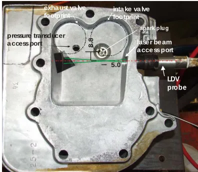
[image:3.595.323.521.85.257.2]The LDV probe and the system used in the present work to collect the data are described in the paper by Esirgemez and Ölçmen [30]. In the present work, single component velocity measurements were made using the two-simultaneous velocity component, miniature LDV probe that was placed in the spark-plug hole of the Briggs and Stratton engine (Figure 1). Data was col-lected by a TSI-FSA-4000 frequency-based processor and reduced by an in-house code to obtain the time varia-tion of a velocity at a locavaria-tion near the spark-plug loca-tion. Probe volume with 70 µm × 70 µm × 1.3 mm size was located 3.6 mm away from the piston when it is at its top-dead-center. Time alignment of the LDV and the engine data was accomplished via an in-house code. Figure 2 shows the experimental data non-dimensional- ized with the maximum value of the ensemble-averaged mean velocity. Positive velocity values indicate flow into the engine, such as the velocity values observed during
Table 1. Briggs and Stratton test engine relevant data.
Model Number 256427
Combustion Chamber Type L Head
Bore [mm] 87.31
Stroke [mm] 66.68
Displacement [cc] 399.3
inta ke va lve footprint exha ust va lve
footprint
spark plug pressure transducer
a ccess port
LDV probe
lase r be am a cce ss port
5.0
8.
8
Figure 1. The combustion bowl, crossing of the schematic laser beams indicate the measurement probe volume. Dis-tances shown have mm units.
the intake stroke (0 - 180 degree range). Experimental data general characteristics were next used to specify the general characteristics of the simulated signal, rather than analyzing the data, similar to the approach taken by Kevlehan et al. [31], where the authors used multiple methods to identify the vortical structures they generated by a test function.
Data was used to calculate the mean velocity values in 1 degree crank angle increments using ensemble averag-ing (see Section 3.1). Difference between the time-de- pendent velocity and the mean velocity at a given crank angle was further used to calculate the standard deviation of the data, data 0.205, (Section 3.1). The data was further used to adjust the standard deviation of the fluctuating component of the simulated signal. Thus measured data was used both to adjust the simulated sig-nal mean and fluctuating velocity sigsig-nals. The experi-mental data was used to aid in defining the simulation signal; the simulation signal was not intended to replicate the experimental data. The data acquisition rate during the experiments was not high enough to capture the fre-quency variation of the signal. Thus the data were plotted as velocity vs. the crank-angle range to obtain the veloc-ity distribution. The data rate also varied with the crank angle resulting in more samples at different crank-angle ranges. Thus this precursory experimental data was used only to define the general characteristics of the simula-tion signal.
2. Signal Generation
[image:3.595.58.286.646.734.2]No
n-di
m
en
sio
nal
v
el
o
ci
[image:4.595.134.461.83.300.2]ty
Figure 2. LDV data and simulated signal mean velocity variation with the crank angle.
and match the variations of the mean and fluctuating components of the simulated signal to the experimental data. Figure 2 shows the simulated mean velocity varia-tion and the collected data. The turbulent part of the sig-nal was generated using a prescribed power spectrum as described in Section 2.2. This approach was taken since the LDV measurement technique results in data that is unequally spaced in time, requiring pre-processing tech-niques prior to the application of the methods discussed in the current paper [32]. Although LDV technique has been employed in unsteady flows for the last three dec-ades, its inherently temporally irregular data acquisition continues to be investigated in obtaining spectrum from such data [33,34].
A data stream of one second duration was simulated for use in the discussion of the analysis methods de-scribed in Section 3 for easiness of presentation of the results. However, the Matlab code written could be used to generate any desired time length of data. Longer dura-tion simulated signal data has been generated and used in further analysis as discussed in Section 4 of the current paper.
2.1. Mean Velocity Signal
A sinusoidal wave with unity amplitude was used as the base signal. The amplitude of the signal was varied to mimic the cycle-to cycle variations that may be observed during an engine run (Figure 3(a)). The signal frequency was chosen as 10 Hz, corresponding to ten crank revolu-tions per second (five full-engine cycles per second), and 600 RPM, a typical idle speed. The period of the signal was kept constant assuming the RPM of the engine does not change during the analysis. Next, Gaussian pulses
were added to vary the signal locally in time similar to the ensemble-averaged mean velocity variation of the experimental data. Gaussian pulses are used since it al-lows signal generation with desired magnitude and bandwidth at a prescribed point in time. Multiple Gaus-sian pulses (yg) were used as needed to effectively define the simulated signal. The simulated mean velocity varia-tion is expressed as:
1 0.1*sin 0.4*
π*
*sin 2*
π*
1 2 3 4 5
U t t t
yg yg yg yg yg
(1)
t 10*t (2)
t denotes the variation of crank angle in time. Gaussian pulses were generated using:
1
2 2 2 2
0.3
*π * *
* exp( )*cos 2*π* *
4*ln 10
c
c
yg C
t td bw f
f t td
(3)
C1 = magnitude, td = time delay, t = time, fc = cut-off
[image:4.595.310.536.652.731.2]frequency, bw = bandwidth of the signal. Five Gaussian pulses together with different parameters were used. The parameters are given in the Table 2.
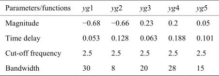
Table 2. Gaussian-modulated sinusoidal pulse parameters.
Parameters/functions yg1 yg2 yg3 yg4 yg5
Magnitude −0.68 −0.66 0.23 0.2 0.05
Time delay 0.053 0.128 0.063 0.188 0.101
Cut-off frequency 2.5 2.5 2.5 2.5 2.5
Figure 3(b) shows the sum of signals yg1 through yg5. The sum of the Gaussian pulse signals and the base sig-nal describing the simulated mean velocity variation in time is shown in Figure 3(c).
2.2. Turbulence Signal
The fluctuating velocity signal was generated using a generic turbulence normalized power spectrum that is also observed in IC engine flow fields,
0 5/3
0 1
1 32*
hw f f
f f
[image:5.595.83.513.511.719.2](4)
[3,27,28,35] and using the Yule-Walker relations [36], where, f is the frequency, f0 is the highest frequency in the spectrum (f0 = 3600 Hz), and “hw” is the normalized power of the signal at a particular f/f0 [37]. The Yule-Walker relations calculate the coefficients of an auto-regressive model (a digital filter) to alter a Gaussian white-noise signal (Figure 4(a)) with a standard devia-tion of unity to obtain a signal with normalized pre-scribed power-spectrum at desired frequencies, such as the frequencies prescribed in the function “hw” given by Equation (4). Once this filter is applied in time domain to a Gaussian white-noise signal, a time-series signal with the prescribed power spectrum is obtained (Figure 4(b)). In the present work, forty-five Yule-Walker filter coeffi-cients were used. Time-domain filter used was a filter that would result in a zero-phase distortion in the filtered signal. A random number generator stream was chosen to generate the Gaussian white-noise so that at every pro-gram run the random number stream would initialize to the same value for the repeatability of the results. The
time step used in signal generation was, t 1 7200 s. Next, modulations were employed on the filtered Gaus-sian signal to simulate cyclic variations that might be present in the fluctuating velocity. It is believed that the cyclic variations in mean quantities would result in cyclic variations of the turbulence in such unsteady flows. Filtered Gaussian white noise amplitude was changed using a modifier signal (Figure 4(c)):
0.2*sin π* 1 *
6 7 8
MS t yg yg yg (5)
The signal is composed of sine modulated Gaussian pulses, where yg6 and yg7 are described by Equation (3), and the parameters given in Table 3.
Cyclic variations were considered since the turbulence transport is directly related to the spatial gradients of correlations and velocity products calculated using the mean and fluctuating velocity values and fluctuating pressure as described by the transport equation for the Reynolds stresses [38]. Effect of unsteadiness on the de-velopment of turbulence has been subject to multiple papers, such as, in accelerating pipe flows [39], pulsating channel flows [38], or flow over airfoils under deep stall conditions [40], where unsteadiness causes unsteady variations in turbulence quantities. Cyclic variations in turbulence were also contemplated by Enotiadis et al., [29]; Fansler, [28]; however no explicit relations were suggested.
Amplitude of the filtered and modified Gaussian noise was next adjusted to match the fluctuating velocity varia-tions observed in the experimental data at different crank angles. For this purpose ensemble averaged standard deviation variation of the experimental fluctuating veloc-ity data with the crank angle was calculated and the fil-tered and modified Gaussian noise amplitude was ad-
0 0.1 0.2 0.3 0.4 0.5 0.6 0.7 0.8 0.9 1
-2 0 2
time (s)
U m
bas
e
0 0.1 0.2 0.3 0.4 0.5 0.6 0.7 0.8 0.9 1
-1 0 1
time (s)
U G
aus
s
0 0.1 0.2 0.3 0.4 0.5 0.6 0.7 0.8 0.9 1
-2 0 2
time (s)
U m
(a)
(b)
(c)
0 0.1 0.2 0.3 0.4 0.5 0.6 0.7 0.8 0.9 1 -4
-2 0 2 4
time (s)
G
auss
ian w
hi
te
noi
se
0 0.1 0.2 0.3 0.4 0.5 0.6 0.7 0.8 0.9 1
-0.5 0 0.5
time (s)
fi
lt
er
ed w
hi
te
no
is
e
0 0.1 0.2 0.3 0.4 0.5 0.6 0.7 0.8 0.9 1
0 0.5 1
time (s)
MS
0 0.1 0.2 0.3 0.4 0.5 0.6 0.7 0.8 0.9 1
-1 0 1
time (s)
u'
10-1 100 101 102 103 104
10-5 10-4 10-3 10-2 10-1 100
frequency (Hz)
pow
er
power~f -5/3
(a)
(b)
(c)
(d)
(e)
[image:6.595.65.531.81.507.2]Figure 4. (a) Gaussian white noise; (b) Filtered Gaussian white noise; (c) Modifier signal; (d) Simulated fluctuating velocity signal; (e) Single sided spectrum of the fluctuating velocity signal.
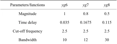
Table 3. Gaussian-modulated sinusoidal pulse parameters used in fluctuating velocity modifier signal.
Parameters/functions yg6 yg7 yg8
Magnitude 1 0.8 0.5
Time delay 0.035 0.1675 0.115
Cut-off frequency 2.5 2.5 2.5
Bandwidth 10 12 30
justed so that the standard deviation of the simulated signal would follow the variations of the experimental data at different crank angle ranges. Overall root-mean- square of the simulated signal and the experimental data were also matched. Turbulence signal is defined as:
filtered Gaussian noise* 0.6 1.8*
u t MS (6)
and has the standard deviation as same as of the original data, data 0.205 (Figure 4(d)). While Equation (5) describes the amplitude modifier signal, the use of it to-gether with Equation (6) allows imposing periodic varia-tions on the fluctuation signal. Single-sided power spec-trum of the fluctuating velocity signal (Figure 4(e)) in-dicates that the power decreases as ~f−5/3, as prescribed by Equation (4), with the effect of amplitude modifica-tions by Equation (5) observed in 100 - 200 Hz range.
2.3. Composite Signal
[image:6.595.58.286.577.663.2]
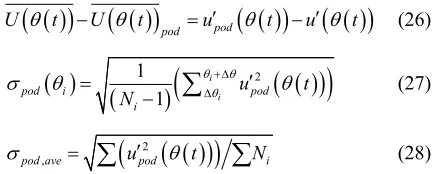
U t U t u t
(7) where,
t, is the crank angle varying in time between 0˚ and 720˚ for a full cycle of a four stroke engine;
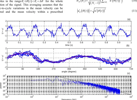
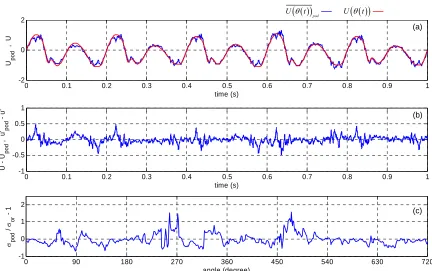
denotes the mean velocity value at a crank angle;denotes the fluctuating velocity. Figure 5(a) shows the composite signal. Figure 5(b) shows the en-semble averaged mean velocity signal and the time- varying signal presented as a function of the crank angle. Single-sided power spectrum of the composite signal is shown in Figure 5(c). The power contained in the fre-quencies above 100 Hz decreases as ~f−5/3.
u t
2.4. Statistical Quantities
The average mean-velocity variation with crank-angle using only the original mean velocity signal is defined as:
i
i
i
U U t
Ni (8) where i denotes the prescribed crank angles at whichthe mean velocity values are calculated, 0,1, 2, , 719 ;
i
1 ;
i t
is the number of
samples in the range i
,
i
N
for the whole duration of the signal. This averaging assumes that the cycle-to-cycle variations in the mean velocity can be ignored and the mean velocity within a prescribed
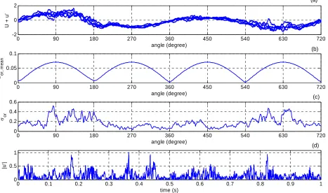
crank-angle range can be represented with a single mean value. Figure 6(a) shows the composite velocity varia-tion with the crank angle.
A standard deviation related to the mean velocity variation is defined using different representations of the mean velocity:
2 or,mean1 1
i
i
i i
i
U t U
N
(9)This value is different than zero due to cyclic variation in the original mean velocity signal (Figure 6(b)). Fig-ure 6(b) indicates that presenting the mean velocity sig-nal with averaged values within crank angle intervals results in the calculation of a standard deviation different than zero, which could be wrongfully interpreted as tur-bulence signal.
The fluctuating velocity signal was next used to obtain the standard deviation at prescribed crank angle intervals, the absolute value of the fluctuating ve-locity, and an overall average standard deviation, given with the following equations, respectively.
u t
2
or1 1
i
i
i
i
u t
N
(10)
2or
u t u t (11)
0 0.1 0.2 0.3 0.4 0.5 0.6 0.7 0.8 0.9 1
-2 -1 0 1 2
time (s)
U +
u
'
0 90 180 270 360 450 540 630 720
-2 -1 0 1 2
angle (degree)
U +
u
'
10-1 100 101 102 103 104
10-5 10-4 10-3 10-2 10-1 100
frequency (Hz)
pow
er
(a)
(b)
[image:7.595.75.539.365.704.2](c)
0 90 180 270 360 450 540 630 720 -2
0 2
angle (degree)
U +
u
'
0 90 180 270 360 450 540 630 720
0 0.05 0.1
angle (degree) or, m
ea
n
0 90 180 270 360 450 540 630 720
0 0.2 0.4 0.6
angle (degree) or
0 0.1 0.2 0.3 0.4 0.5 0.6 0.7 0.8 0.9 1
0 0.5 1
time (s)
|u'
|
(a)
(b)
(c)
[image:8.595.65.532.91.367.2](d)
Figure 6. Simulated signal statistics: (a) Signal velocity distribution with crank angle; (b) Mean velocity standard deviation (Equation (9)) calculated using the original mean and the ensemble averaged mean velocity; (c) Standard deviation variation with the crank angle; (d) Absolute value of the fluctuating velocity in time.
2
or,ave u t Ni
(12)where or
i describes an ensemble averaged varia-tion of the fluctuating velocity signal (Figure 6(c)), theor,ave
defines a single standard deviation value for the fluctuating velocity signal (or,ave 0.205 for the
cur-rent signal). The uor shows the variations of the signal
from the mean in the absolute sense (Figure 6(d)).
3. Analysis Methods-Description/Discussion
Different methods used in the analysis of the simulation signal were, ensemble averaging, high-pass filtering, Proper Orthogonal Decomposition (POD) also known as Principal Component Analysis (PCA) [41], Wavelet De-composition (WD), WD and PCA together (WD/PCA). In this section these methods are described and some analysis results about their use are given.
Methods discussed in this section are the most com-monly used methods in the analysis of cycle-to-cycle variation of engine data. Usually multiple techniques are employed within the same research. While the ensem-ble-averaging method is the most commonly used me- thod [5,27,42-45], high-pass filtering method has been frequently employed [22,27,28,44-46]. Literature survey indicates that POD, WD and the WD/PCA methods have
been less frequently employed [3,18,20-25].
Previous research on cyclic variability indicates that the time varying velocity in highly unsteady IC engine flows has usually been expressed as sum of mean and fluctuating components, U t
U t( )?u t
. In general, the mean velocity component is considered as the com-ponent causing the cyclic variability in the signal; al-though cyclic variability in the fluctuating velocity has also been contemplated [28,29]. The methods used by different researchers differ in how the mean and the fluctuating velocities are determined.In ensemble-averaging method it is assumed that the mean velocity does not vary from one cycle to the next and arithmetic averages of the velocities at specified crank angle intervals can be used to describe the mean velocity variation,
en en
In the high-pass (hp) filtering method [27], (named as “cycle resolved analysis” by Liou and Santavicca, [44] and Fraser and Bracco [45]; named as “cyclic averaging” by Sulivan et al. [22], time varying velocity signal is filtered at a pre-determined cut-off frequency to calculate the low-pass (lp) filtered signal and this signal is referred to as the mean velocity signal,
U t U u t .
hp
U t U t u t
lp . A variant of this
Another variant of high-pass filtering method, named as “filtered ensemble averaging” by Fansler [28] (named as “phase averaging”, Erdil et al. [3]), uses three terms to describe the velocity signal. In this method the difference between the low-pass filtered velocity and the ensem-ble-averaged mean velocity is defined as low frequency (LF) fluctuating velocity and the u’(t) is then considered as composed of a high frequency (HP) component,
LF
HP
U t U enu t u t . In this vari-ant the mean velocity is defined as,
en en LF
U t U u t
, and the fluctuating veloc-ity as, . In essence high-pass filtering and the filtered ensemble averaging methods are equiva-lent to each other, and in each method different cut-off frequencies could be used at each cycle; although usually one frequency is used for the whole signal.
HP
u t u t
In the WD method the velocity signal is decomposed into “details”, where the sum of the details gives the ori- ginal velocity signal. The fluctuation velocity informa-tion contained in the “detail” decreases with the increas-ing “detail” level. In this technique a high order “detail” is considered as the mean velocity signal.
In the POD method, velocity signal is re-expressed using new axes found as the eigenvectors of a covariance matrix formed using the velocity signal. The eigenvec-tors and the associated eigenvalues describe new coordi-nate axes on which the data lie the closest; the larger the eigenvalue the closer the data is to the eigenvector. In a reverse transformation to the original axes, neglecting the variations of signal along the axes with low eigenvalues allows defining the mean velocity component. In the WD/PCA method first the velocity signal is decomposed into details and then the POD is applied on these details. Similar to the WD method a high order detail is then considered as the mean velocity signal.
Additional unique methods, such as “turbulence filter-ing” by Erdil et al. [3], discuss possibility of separating the mean and the fluctuating velocities within the fquency domain using a filter function. In the current re-search, both the mean and the fluctuating velocities were considered to be time dependent and both were consid-ered to have cyclic variations. In each method fluctuating velocity signals were next used to study turbulence sta-tistics.
3.1. Ensemble Averaging
In the ensemble averaging method, time dependent ve-locity is defined as the sum of the ensemble-averaged mean velocity and the fluctuating velocity:
i en en
U t U u t
(13) where,
t , is the crank angle;
denotes average value; i, are the prescribed crank angles at which themean velocity values are calculated. Ensemble averaging assumes that the mean flow variation from one cycle to another is negligible and an average velocity value can be used to represent the mean value at a crank angle. The average velocity at a crank angle is calculated as the arithmetic mean of the velocity values within a pre-scribed crank angle interval:
i
i
i en
i
U t
U
N
(14)0,1, 2, , 719
i
; 1; is the number of samples in the range
,
i
N
ti i
for the whole duration of the signal. The U
i en (Equation (14)) is different than the U
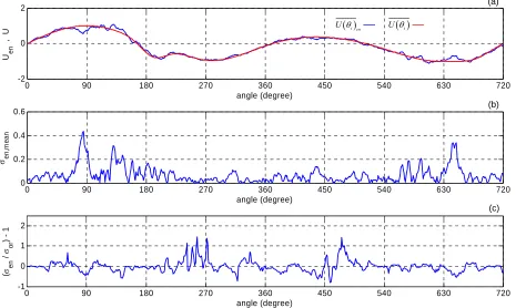
i (Equation (8)), since theen-semble averaged mean velocity is obtained using the composite signal rather than the mean velocity variation alone. Figure 7(a) shows both ensemble averaged mean- velocity variations calculated using the composite signal and using only the mean component of the composite signal (shown as smooth line).
A standard deviation is calculated using the differ-ences between the ensemble-averaged mean velocity and the mean velocity of the original signal at the prescribed crank angles using the whole duration of the signal as:
,mean
2
1
( 1)
i
i
en i
i en i
U t U
N
(15)
Figure 7(b) shows the en,mean
i variation calcu-lated using Equation (15). The variation shown is differ-ent than the variation shown in Figure 6(b) calculated using Equation (9) due to the differences in the mean velocity definitions used. Figure 7(b), as Figure 6(b), indicates to the fact that ensemble averaging results in large velocity fluctuations due to predicting the mean velocity variation incorrectly by ignoring cycle-to-cycle variations. The difference between the original signal mean and the ensemble mean (Equation (14)) results in a fluctuating signal.The fluctuating velocity is next used to obtain standard deviation of the fluctuating velocity at prescribed crank angles:
1
2
1i
i
en i en
i
u t
N
(16)A standard deviation, en ave, using the whole signal is calculated by:
,
en ave u t Ni
(17)0 90 180 270 360 450 540 630 720 0
0.2 0.4 0.6
angle (degree) en
,m
e
an
0 90 180 270 360 450 540 630 720
-1 0 1 2
angle (degree)
(
en
/
or
) - 1
0 90 180 270 360 450 540 630 720
-2 0 2
angle (degree)
U en
, U
i en
U — U i
(a)
—
(b)
(c)
Figure 7. (a) Ensemble averaged mean velocity variations, U
i en and U
i ; (b) en,mean
i given by Equation (15); (c)Difference between en
i and the or
i nondimensionalized by or
i .deviations for the fluctuating velocities normalized by the standard deviation of the original signal.
In the application of the technique, simulated data with prescribed durations were used to calculate the mean velocity and the standard deviation variation with crank angle. Calculated variations for different signal durations differ from each other since the simulated signal contains cyclic variations that affect the calculated values. Calcu-lation of the mean and the standard deviation variation by averaging the data values over the span of the signal rules out the use of the technique to obtain time-resolved variations.
3.2. High-Pass Filtering
In the high-pass filtering method the simulated signal is split into high and low frequency components at a cut-off frequency, fc, chosen by observation (fc = 30 Hz). The
time dependent signal is low-pass filtered to obtain the mean velocity variation in time,
low pass (Figure
8(a)). The difference between the original signal and the low-pass filtered signal is considered to be the fluctuat-ing velocity signal.
U t
low pass hpf
U t U t u t
(18)In the present work a single frequency value is used
for the full length of the signal to separate the low and the high frequency contents. A Fast-Fourier-Transform is applied to the original signal to determine the power spectrum of the signal and to subsequently determine a cut-off frequency. The original time series signal was next filtered using a sixth order Chebyshev filter in the time domain to obtain the low frequency component. A relation exists between the mean velocity differences and the fluctuating velocity differences calculated using the original velocity signal and the velocity signals calcu-lated by the method:
low pass hpf
U t U t u t u t (19)
Velocity differences are presented in Figure 8(b). High frequency signal was then used to calculate the fluctuating velocity standard deviation at different crank angles, and an overall average standard deviation:
1
2
( 1)i i
hpf i hpf
i
u t
N
(20)
2
,
hpf ave uhpf t i
N (21)Cut-off frequency fc = 30 Hz, results in hpf ave, = 0.1957. Different cut-off frequency values result in dif-ferent hpf ave, values; for fc = 10, 15, 20, and 25 Hz, the
[image:10.595.69.534.89.367.2]0 0.1 0.2 0.3 0.4 0.5 0.6 0.7 0.8 0.9 1 -1
-0.5 0 0.5 1
time (s)
U
U
lo
w
p
a
s
s
, u
' hp
f
- u
'
0 90 180 270 360 450 540 630 720
-1 0 1 2
angle (degree) hp
f
/
or
- 1
0 0.1 0.2 0.3 0.4 0.5 0.6 0.7 0.8 0.9 1
-2 0 2
time (s)
U low
pas
s
,
U
(a)
(b)
(c)
low passU t — U
t
—Figure 8. (a) Mean velocity variation obtained using high-pass filtering method and the simulated signal mean velocity
varia-tion (solid line in red); (b) Variavaria-tions of U
t
U
t
low pass , and uhpf
t
u
t
with time; (c) Differencebetween hpf
i and the or
i nondimensionalized by or
i .0.2223, and 0.2129, respectively. With the use of a 5 second long signal the values obtained for the fc = 10, 15,
20, 25 and 30 Hz, are hpf ave, = 0.2604, 0.2119, 0.2102, 0.1954, 0.1788 respectively, indicating that the signal length does have an effect on the values calculated, but the effect is not significant at high frequency end.
Figure 8(a) shows the mean velocity calculated by the high-pass filtering technique and the mean velocity varia- tion of the original signal in time. Figure 8(c) shows the difference between the standard deviations for the fluctu-ating velocities normalized by the standard deviation of the original signal.
3.3. Proper-Orthogonal Decomposition (POD)
The proper orthogonal decomposition (POD) was first introduced by Lumley [48] to identify coherent structures in turbulent flows. POD, also known as the Principal Component Analysis technique [41] allows one to repre-sent data points each defined with N coordinates in a new N dimensional coordinate system such that the data points now lie closer to the new axes, allowing variations along preferred directions to be determined [49]. For example data maybe the realization of three fluctuating velocity components obtained in time, where the
fluctu-ating velocities are the coordinates defining the data point obtained in time. In the representation of the data in the new coordinate system, the axes are sorted such that the data lie closer to the first axis than the other axes and the data lie closer to the second axis than to the third axis and so on. Representation with the new variables is sometimes referred to as sorting the data by their energy content. One of the advantages of the POD technique is that after the representation of the data in the new coor-dinate system, one can then approximate the data by re-ducing the number of coordinates used, say by neglecting the less energetic coordinates in representing the data. For more details and examples of POD technique on fluid mechanics measurements, the reader is referred to Tropea et al. [50].
In the numerical calculations of the POD technique multiple signals collected simultaneously are first stored in a data matrix, Xi j, , and the data matrix is then used to calculate a covariance matrix.
,
,
* ,T i j i i j i
Cov i j X X X X
(22)where, Xi denotes the average of the data values in the ith row, thus
i
[image:11.595.75.523.87.365.2]covari-ance matrix, Cov i j
, is an M × M square matrix. The next step is calculation of the eigenvalues and the eigenvectors of the covariance matrix. Eigenvalues, k,where k = 1 to M, and the eigenvector matrix i k, , where
i = 1 to M and k = 1 to M, of the covariance matrix, are calculated using Matlab. An eigenvector corresponding to an eigenvalue,
V
k
is listed in the kth column of the eigenvector matrix i k, . The eigenvectors of the covari-ance matrix correspond to the set of orthogonal axes (new coordinates) to represent the data. Once the vectors are sorted in order corresponding to the eigen-values of the covariance matrix, the projection of the original data along the eigenvector directions represents the data in these new orthogonal coordinates. During the process the sum of the square of the distances between the new axes (along the eigenvector directions corre-sponding to eigenvalues in descending order) and the data are minimized.
V
Projection of the original data along the direction of the unit eigenvectors can be obtained using:
, * i j, i
Ti k
Proj V X X (23)
This process can be reverted to obtained the original signal Xi j, , and can be recalculated using:
, ,
i j i k* , * ,
T
i k i j i i
X V V X X X (23)
The computations in Equation (24) also work if some of the eigenvectors corresponding to less energetic ei-genvalues are omitted (set to zero) during the reversal process, leaving behind a signal close to the original sig-nal that has been cleaned of outlier data points.
In the present work, first the complete velocity signal was converted into a data matrix, Xi j, , with each row of the matrix representing a full cycle of a four stroke en-gine spanning 720˚ of crank angle, with the first 720˚ signal (corresponding to the first cycle) in the first row, next 720˚ signal in the next row and so on. In describing
,
i j
X , i = 1 to M, where, M represent the number of cy-cles used in the signal and j = 1 to N representing col-umns of the data corresponding to one full cycle of data spanning 720˚ of crank angle. Although this is strictly different than the conventional use of the POD technique, it allows working with a single dimensional data. Thus the data matrix is generated as if different cycle veloci-ties were acquired simultaneously, resulting in velociveloci-ties corresponding to same crank-angle to be listed in a single column. Presenting one dimensional data in an array al-lows using each cycle velocity value as a separate coor-dinate in the POD process.
In the present work the mean velocity signal was cal-culated using the largest eigenvalue containing 92.2% of the energetic contributions to the signal (Figure 9(a)) and the contributions from other eigenvalue/eigenvector couples were considered as turbulence contributions. The
five eigenvalues obtained in the increasing order are 108.6, 150, 236.7, 280.9, and 2735.7. The contributions for the eigenvalues for a 10 second signal results in 50 eigenvalues, and the approximation improves with the simulated signal duration (discussed in Section 4.1).
In the POD method time dependent velocity is defined as the sum of the mean and the fluctuating velocity components:
pod pod
U t U t u t
(25) Statistical quantities are defined similar to other method statistical quantities:
pod pod
U t U t u t u t
(26)
1
2
1i
i
pod i pod
i
u t
N
(27)
2
,
pod ave upod t i
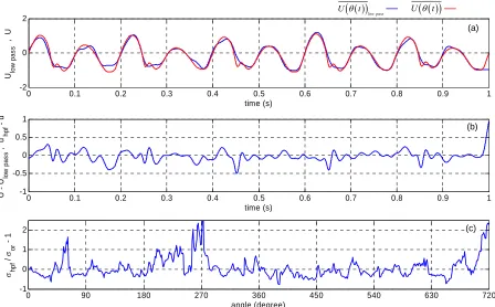
N (28)Figure 9(b) shows the difference between the mean velocities and the fluctuating velocities for the original signal and the ones calculated by the POD technique. Figure 9(c) shows the difference between the standard deviation calculated using the POD technique and stan-dard deviation of the original fluctuating velocity nor-malized by the standard deviation of the original signal.
3.4. Wavelet Decomposition
Wavelet transformation determines the correlations be-tween the original signal and the prescribed wavelet function at different frequency ranges of the original signal [51]. Following the description used by Farge [52] continuous wavelet transform is defined as the convolu-tion of a wavelet ( ) t , with the original signal to deter-mine the wavelet coefficients,
,
a b,
C a b
f t t td (29) where
1/2 ,a b
t b
t a
a
(29)
“a” denotes the scale of the wavelet and related to the frequency of the signal, “b” is time value used in trans-lating the wavelet; a b,
t is the daughter waveletsgenerated by translating and dilating (scaling) the mother wavelet. The wavelet coefficients thus calculated can be used to approximate the original signal at different scales. Reconstruction of the original signal is obtained using linear combination of the wavelet and the wavelet coeffi-cient
1
2 , , a b [image:12.595.323.539.239.326.2]0 0.1 0.2 0.3 0.4 0.5 0.6 0.7 0.8 0.9 1 -1
-0.5 0 0.5 1
time (s)
U
U
po
d
,
u
' pod
-
u
'
0 90 180 270 360 450 540 630 720
-1 0 1 2
angle (degree)
po
d
/
or
- 1
0 0.1 0.2 0.3 0.4 0.5 0.6 0.7 0.8 0.9 1
-2 0 2
time (s)
U po
d
,
U
(a)
(b)
(c)
podU t — U
t
—Figure 9. (a) Mean velocity variation obtained using the POD and the simulated signal mean velocity variation (solid line in
red); (b) Variations of
pod
U t U t
- , and upod
t
u
t
with time; (c) Difference between pod
i andthe or
i nondimensionalized by or
i .where C , is a constant and depends on the wavelet used. The coefficients with small scale values correspond to high frequency component of the signal and the ones with larger scale values correspond to low frequency values. During the reconstruction of the signal, length scales corresponding to the high frequency content can be omitted to obtain the low frequency (or mean) varia-tion of the original signal. A history and a formal de-scription of the wavelet transforms can be found in arti-cles by Farge [53] and Tropea et al. [50].
,
1 2 t b dC a b f t a t
a
(32)where and the
transformation gives the wavelet coefficients,
2 ,j * 2 . 1, 2, , 1, 2 ,j
a b k j k
, , C a b . The original signal can be recovered without any loss using the inverse transform:
, j k,
j k
f t
C j k t (31)While the mother wavelet can be presented in a func-tional form for a simple wavelet such as the Haar wavelet, in general an algebraic functional form does not exist. The mother wavelet , which can be a real or com-plex valued function, is chosen to satisfy multiple condi-tions, such as admissibility condition requiring that the energy contained within the wavelet to be a limited value, zero mean condition requiring the wavelet to have a zero mean value, and a requirement that its higher order mo-ments vanish [53].
t For a fixed value of j, summation on the k gives the “detail” at the jth level:
, ,
jk
D t
C j k j k t
(34)and thus,
j j
f t
D t (35)An approximation to the signal can be made using a limited number of details. For example f t
can be separated into two components, one using indices j≤ J, corresponding to the scales, a2j2J and one with j> J. In the discretized wavelet transform the scale and the
position “t” are described using powers of 2. Matlab [54] gives details about the discrete wavelet transform and the reader is referred to this document for further details. For a continuous signal f t
, the discrete wavelettrans-form is given
j J j
j J j
J j J j
f t D t D t A D
t (36) [image:13.595.81.513.83.354.2]If desired, the reconstructed signal could then be ex-pressed only as “approximation”, Ai, at level J. A relation
exists between different approximations as:
1
J J j J
A A D (37)
Increasing values of J indicates that lesser details are used in generating the approximate signal, thus the approximation becomes closer to signal’s mean variation. The value of J should also not be chosen large such that the details in the mean variation are also sacrificed.
In the current work Daubechies 12, Symlet 8, and Coiflet 5 wavelets were tested and the results obtained did not vary with the use of different wavelets. Thus Daubechies 12 wavelet was chosen for further analysis of the data. Figure 10 shows the scaling and the wavelet functions for the Daubechies-12 wavelet.
In the wavelet decomposition time dependent velocity is thus defined as an approximation plus the details:
wd wd
U t U t u t
(38) where U
t
wd A uJ, wd
t
j J D tj
, and J =8. Figure 11(a) presents the U
t
wd A8 and the original mean velocity variation in time.Statistical quantities are calculated using:
wd wd
U t U t u t u t
(39)
1
2
( 1)
i
i
wd i wd
i
u t
N
(40)
2
,
wd ave uwd t Ni
(41)Figure 11(a) shows the original mean velocity and the mean velocity calculated by the WD technique. Figure 11(b) shows the mean and the fluctuating velocity dif-ferences, Figure 11(c) shows the difference between the standard deviation calculated using the WD technique and standard deviation of the original fluctuating velocity
normalized by the standard deviation of the original sig-nal.
3.5. Principal Component Analysis and Wavelet Decomposition
In this analysis method the advantages of the Principal Component Analysis and the Wavelet Decomposition methods are used simultaneously [55]. In the technique first wavelet decomposition is applied on the signal to calculate the “details” and one “approximation” to the signal. Next PCA analysis is employed on each of the detail signals and the approximation. PCA analysis re-sults are used to determine which principal components to keep in the signal using the Kaiser rule. Kaiser rule keeps only the eigenvalues, which have values greater than the mean of all eigenvalues in re-construction of the signal. As a next step the details and the approximation reconstructed using the PCA are used in the reconstruc-tion of the signal using the wavelet decomposireconstruc-tion. In the detection of the mean velocity signal the wavelet de-composition allows the signal to be analyzed at different scales and the principal component analysis allows de-noising of the signal at every detail.
In the WD/PCA method time dependent velocity is defined as the sum of the mean and the fluctuating veloc-ity components,
wdpca wdpca
U t U t u t
(42)Statistical quantities are defined using,
wdpca wdpca
U t U t u t u t
(43)
1 1
2
i
i
wdpca i wdpca
i
u t
N
(44)
2
,
wdpca ave uwdpca t i
N (45)0.5
0
–0.5
0 5 10 15 20 0 5 10 15
0.8
0.6
0.4
0.2
0
–0.2
–0.4
(a) (b)
[image:14.595.70.289.316.473.2] [image:14.595.80.287.393.471.2] [image:14.595.87.540.406.724.2]0 0.1 0.2 0.3 0.4 0.5 0.6 0.7 0.8 0.9 1 -1
-0.5 0 0.5 1
time (s)
U
U
wd
,
u
' wd
-
u
'
0 90 180 270 360 450 540 630 720
-1 0 1 2
angle (degree) wd
/
or
- 1
0 0.1 0.2 0.3 0.4 0.5 0.6 0.7 0.8 0.9 1
-2 0 2
time (s)
Uwd
,
U
(a)
(b)
(c)
wdU t — U
t
—Figure 11. (a) Mean velocity variation obtained using the WD and the simulated signal mean velocity variation (solid line in
red); (b) Variations of U
t
U
t
wd, and uwd
t
u
t
with time; (c) Difference between wd
i andthe or
i nondimensionalized by or
i .Figure 12(a) shows the original mean velocity and the mean velocity calculated by the WD technique. Figure 12(b), shows the mean and the fluctuating velocity dif-ferences, Figure 12(c) shows the difference between the standard deviation calculated using the WD/PCA tech-nique and standard deviation of the original fluctuating velocity normalized by the standard deviation of the original signal.
4. Results and Further Discussion
A comparison between the Figures 8(a), 9(a), 11(a),and 12(a) show that all the mean velocity variations calcu-lated by different methods follow the general variations observed in the simulated signal. Figures 8(b), 9(b), 11(b), and 12(b) show the differences of the mean and the fluctuating velocities between the original velocity components and the components calculated after each method, and give a sense of how well the methods per-form in describing both the mean velocity and the fluctu-ating velocity vs. the crank angle. If a method could per-fectly separate the mean and the fluctuating velocity val-ues in time then the plots would be a straight line at zero. Figures indicate that the differences between the velocity
signals are the smallest using the WD/PCA method, and that the POD method results contain high frequency con-tent. POD performance improves with increased signal duration and the high frequency diminishes.
Figures 7(c), 8(c), 9(c), 11(c), and 12(c) show the normalized difference between the computed and the original signal standard deviations. Figures 8(c) and 11(c) indicate that the high-pass filtering and the WD tech-niques result in larger differences between the standard deviations than the other methods. The differences be-tween the fluctuating and the mean velocities obtained using the original simulated velocity signal and the ve-locities computed after each method both contribute in the calculation of the fluctuating velocity standard devia-tion. This is due to the fact that the difference between the original velocity signal and the calculated mean ve-locity signal is considered as a contribution to the fluc-tuation velocity calculated by a method. For the 1 second analysis results shown in the figures, large non-dimen- sional differences are observed at locations where the original or
i values are small such as in the 250˚ - 280˚ and 450˚ - 500˚ ranges. Overall, the WD/PCA tech-nique results follow the original standard values better [image:15.595.70.527.83.371.2]
0 0.1 0.2 0.3 0.4 0.5 0.6 0.7 0.8 0.9 1
-1 -0.5 0 0.5 1
time (s)
U -
Uw
dpc
a
,
u'w
dpc
a
-
u'
0 90 180 270 360 450 540 630 720
-1 0 1 2
angle (degree) wdpc
a
/
or
- 1
0 0.1 0.2 0.3 0.4 0.5 0.6 0.7 0.8 0.9 1
-2 0 2
time (s) Uw
dpc
a
,
U
(a)
(b)
(c)
wdpcaU t — U
t
—time (s)
time (s)
angle (degree)
Figure 12. (a) Mean velocity variation obtained using the WD/PCA and the simulated signal mean velocity variation (in red);
(b) Variations of U
t
U
t
wdpca, and uwdpca
t
u
t
with time; (c) Difference between wd pca
i andthe or
i nondimensionalized by or
i .4.1. Simulated and Calculated Signal Correlation —Effect of Signal Duration
In order to quantitatively determine the performance of each method in separating the mean and the fluctuating velocity variations, and the signal duration required to effectively separate the mean and the fluctuating velocity signal components correlation coefficients were calcu-lated between the original simulation signal and the cal-culated signals. Correlation coefficients were calcal-culated using:
method
mean 2
method *
corr coeff
*
U t U t
U t U t
2
(46)
and
method
fluc 2 2
method *
corr coeff
*
u t u t
u t u t
(47)
A correlation coefficient of 1 indicates a perfect match between the two signals. Correlation coefficients calcu-lated for signal durations of 0.6 s to 10.2 s with 0.6 s in-crements plotted in Figure 13 indicate that the WD/PCA method performs better than the other methods in calcu-lating the mean and the fluctuating velocity signals. Both Figures 13(a) and (b) indicate that the performance of the methods get better with increased signal duration. Results do not show appreciable improvement after the first 3 seconds, and the changes after 8 seconds are
[image:16.595.104.498.86.295.2]minimal indicating that 3 seconds of data could be suffi- cient to extract the mean and the fluctuating velocity signals. Plots in Figures 13(a) and (b) show similar variations since poor mean velocity prediction by a method directly reflects on the fluctuating velocity prediction performance of the technique. Results also indicate that the WD and the high-pass filtering methods predict the mean and the fluctuating velocity variations poorly even with increased signal duration. Correlation coefficients as low as 0.8 obtained for the fluctuating signal indicate that the time variation of the fluctuating velocity calculated by these methods is a poor representation of the original fluctuating velocity signal. Figure 13(b) shows that the correlation coefficient values calculated even with the WD/PCA method is about 0.95 indicating to the need for further improved methods for accurate time variation prediction of the fluctuating velocity signal.
Figure 14 shows the ratio of the average standard de-viations calculated by each method to the original signal average standard deviation for a given duration of signal. Normalized standard deviation (NSD) was calculated using:
method, or,
Normalized standard deviation
ave ave
[image:16.595.57.289.498.611.2] (48)
Figure 14 indicates that the standard deviation calcu-lated by the WD/PCA method is approximately the same as the or,ave once a 5 s signal duration is used. All the