Reward and Feedback in the Control over Dynamic Events

ISSN Print: 2152-7180

Reward and Feedback in the Control over

Dynamic Events

Magda Osman, Brian D. Glass, Zuzana Hola, Susanne Stollewerk

Queen Mary University of London, London, England

Abstract

On what basis do we learn to make effective decisions when faced with inter-mittent feedback from actions taken in a dynamic decision-making environ-ment? In the present study we hypothesize that reward information (financial, social) may provide useful signals that can guide decision-making in these situations. To examine this, we present three experiments in which people make decisions directly towards controlling a dynamically uncertain output. We manipulate the framing of incentives (gains and losses) and the form of the incentives (financial, social), and measure their impact on decision-mak- ing performance (both in frequent and intermittent output feedback condi-tions). Overall, performance suffered under intermittent output feedback. Relative to social rewards, financial rewards generally improved control per-formance, and a gains framing (financial, social) leading to better perfor-mance than a losses framing (financial, social). To understand how rewards affect behavior in our tasks, we present a reinforcement learning model to capture the learning and performance profiles in each of our experiments. This study shows that information regarding incentives impacts the levels of exploration, the optimality of decisions-making, and the variability in the strategies people develop to control a dynamic output experienced frequently and intermittently.

Keywords

Intermittent vs. Frequent Feedback, Rewards, Outcome Feedback, DynamicDecision-Making, Uncertainty, Control

1. Introduction

Many of the control based-decision-making situations that we face in the real world are non-stationary. This means that the outputs we are trying to control change state from one moment to the next, which requires us to react and adapt How to cite this paper: Osman, M., Glass,

B. D., Hola, Z., & Stollewerk, S. (2017). Reward and Feedback in the Control over Dynamic Events. Psychology, 8, 1063-1089.

https://doi.org/10.4236/psych.2017.87070

Received: March 23, 2017 Accepted: May 24, 2017 Published: May 27, 2017

Copyright © 2017 by authors and Scientific Research Publishing Inc. This work is licensed under the Creative Commons Attribution International License (CC BY 4.0).

our decision-making on a regular basis (Brehmer, 1992; Osman, 2010). Non- stationary environments are especially difficult to make decisions because we often face uncertainty regarding the source of change to the output, and this un-certainty is exacerbated when the output feedback itself is only experienced in-frequently. In real terms this means that we have to make decisions without re-liably knowing the consequences of our actions at the time the decision is made

(Osman, 2014;Sterman, 1989).

In the essence then, the present study includes three experiments, each of which are designed to reveal how reward information (social, financial) might be a candidate for guiding decision-making when controlling a dynamic output that is either experienced infrequently and frequently. To consider the role of reward information on decision-making, and how it may facilitate decision- making in general, but also under conditions of extreme uncertainty, we discuss two literatures: judgment and decision-making work on intermittent vs. fre-quent feedback, and incentive-based decision-making. In addition, we present theoretical and computational models of decision-making under uncertainty as a basis on which hypotheses are generated, and which also informs the model (SLIDER, Osman, Glass, & Hola, 2015) we utilize in this study.

1.1. Judgment and Decision-Making Work on Intermittent vs.

Frequent Feedback

reacting to output changes. However, as Lurie and Swaminathan (2009) com-mented, it isn’t clear how performance related incentives may have interacted with the frequency with which output feedback was presented.

Intermittent Output Feedback in the Present Study

In the present study we aim to address the issue highlighted by Lurie and

Swa-minathan (2009) by examining the extent to which incentivizing control

per-formance (in which we present reward information on every trial) is affected by infrequent (every 5th trial) or frequent output feedback (every trial). The reward scheme we introduce in our study is less informationally rich than output feed-back. That is, reward information only indicates generally whether one is further or closer to target by a lot or a little, but not precisely how much; whereas output feedback provides precise details in this regard. Therefore, a tentative hypothesis would be that, relying on reward information to learn about the effectiveness of one’s decision-making strategies in an infrequent output feedback condition should lead to poorer performance than when the output feedback is presented frequently, because reward information is less precise than output feedback. However, based on prior studies (Frederickson et al., 1999; Lurie & Swamina-than, 2009), a more general hypothesis is that, compared to frequent feedback, intermittent feedback should lead to better decision-making performance in our dynamic decision-making task.

1.2. The Role of Rewards in Judgment and Decision-Making

Work in decision sciences (incl., psychology, behavioral economics, economics, management) has often shown that the presentation of monetary incentives can actually have a detrimental rather than corrective or positive effect on deci-sion-making performance (for review seeKamenica, 2012). The speculation is that financial incentives interfere with personal intrinsic motivations to perform a given task (Ariely, Gneezy, Loewenstein, & Mazar, 2009;Bahrick, 1954; Eisen-berger & Cameron, 1996; Kamenica, 2012; Lepper, & Greene, 2015; McGraw, 1978;Deci & Ryan, 1985). This is often referred to as the crowding out effect

(Deci, 1976;Frey, 1997;Lepper & Greene, 2015). Moreover, there is evidence to suggest that monetary incentives alone are not sufficient, and need to be pre-sented in combination with output feedback in order to improve deci-sion-making performance(Buchheit et al., 2012). To complement this, an asso-ciation has been made between monetary rewards and expertise such that the greater the skill required to perform the decision-making task accurately the less likely financial incentives positively impact on performance (Vera-Munoz, 1998).

Ortmann, 2001;Smith & Walker, 1993). There is an implicit assumption that the link between rewards and performance is based on a mechanism by which re-wards increase effort, which in turn improves performance (Bonner & Sprinkle, 2002;Buchheit et al., 2012). But, what counts as reliable metrics of cognitive ef-fort is by no means settled (for discussion see Bonner and Sprinkle, 2002). Addi-tionally, the difficulty with providing a more specific answer is that the judgment and decision-making tasks in which financial incentives are used vary in “effort”, i.e., time taken to complete, difficulty, skill, and complexity. Therefore, without any predefined description of mental effort that can be applied to a deci-sion-making task, it is hard to generate precise predictions regarding the relative improvement of performance based on financial rewards. Moreover, given the empirical landscape regarding the role of rewards in decision-making, it is not clear as to whether rewards do reliably lead to improvements in performance.

Reward Schemes in the Present Study

re-ward is based on the accuracy of their control performance (closer to target = 10 points gained, further away from target = 5 points gained). In the financial set up, the rewards are presented as money, in the social rewards set up participants still have the same payoff structure, but the rewards are framed socially (Expe-riments 2 and 3). In the losses/negative conditions participants start off with a lump sum, but they will always lose money, but the amount they lose is depen-dent on their control performance (closer to target = 5 points lost, further away from target = 10 points lost). We predict that, if the regulatory fit literature ge-neralizes to dynamic decision-making tasks, then when there is a fit between global (i.e., task goal, which in dynamic control is promotion-based) and local rewards (i.e., financial gains/positive social rewards), then we would expect more exploratory behaviors and better overall decision-making performance, when there is a mismatch with the local reward structure (financial losses/negative so-cial rewards), for which we expect more exploitative behaviors, which we discuss in more detail in the next section.

1.3. Computational Modeling of Dynamic Decision-Making

The aim here is to ground the proposed computation model within computa-tional work that has been developed to account for behavior in dynamic con-trol-based decision-making tasks. From this we introduce the Single Limited Input, Dynamic Exploratory Response Model (SLIDER, Osman, Glass, & Hola, 2015). At the heart of most computational models of dynamic decision- making is a reinforcement learning component. For example, Le Pelley (2004) presents a hybrid model which uses associative knowledge accrued from prior experience to shape learning in a novel training episode. Erev and Roth (1998) demonstrate that simple reinforcement learning models can describe human performance in dynamic games. In turn, at the heart of all reinforcement learning models is a memory mechanism which updates as a function of prediction error-that is, the discrepancy between a predicted output and the observed output (Sutton &

Bar-to, 1998). Beyond a mathematical description of behavior, neurophysiological

evidence attributes a reinforcement learning role to underlying neural mechan-isms (specifically to regions located in the ventromedial prefrontal cortex; Chase, Kumar, Eickhoff, & Dombrovski, 2015). Thus, reinforcement learning is a criti-cal and useful abstraction of human decision making.

In addition to reinforcement learning, human behavior in dynamic decision making scenarios has been characterized using computational models which in-stantiate the combination or interaction of two or more cognitive mechanisms

(Cisek, 2006). For example, Experience-Weighted Attraction (EWA) models

learning decay mechanism. For this reason, the present paper will utilize a learning decay mechanism in the computational modeling procedure.

The CLARION model, which has been most commonly applied to dynamic decision-making tasks, uses a combination of sub-symbolic representation in the form of hidden neural network layers with back-propagation reinforcement learning (implicit) and symbolic goal representation and attentional control (ex-plicit) (Brooks, Wilson, & Sun, 2012; Sun, Slusarz, & Terry, 2005). The rein-forcement learning mechanisms in CLARION are parameterized with learning weights which are modified with higher level systems which act as attentional control mechanisms within the model. Below, we will specify a computational model which similarly combines reinforcement mechanisms using a variable gating procedure. In addition, Gibson (2007) utilized a two-stage model com-bining connectionist learning with explicit hypothesis testing processes as a means to characterize transfer effects in dynamic decision making from sub- symbolic to symbolic processes. Such hybrid models have been used to model the way decision making systems cope with uncertainty, which is often characte-ristic of dynamic decision-making environments.

Using unsupervised associative learning via self-organizing maps (SOMs),

Van Pham, Tran, and Kamei (2014) developed learning models which cope with

financial uncertainty. The model learned to deal with financial uncertainty which arises from stock-market fluctuations. These fluctuations represent a sin-gle output value (for one particular traded stock) which results from myriad complex and dynamic underlying factors. The decision maker must learn to ad-just their strategy over time in order make effective decisions based on the single value as it fluctuates over time. Similarly, the present set of experiments involves a task in which there is a single output value which represents the summation of various hidden factors in the decision-making environment. The success of a hybrid reinforcement learning model in assessing fluctuating market values over time is an indication that reinforcement-based decision models with an explora-tion-exploitation meta-decision component may offer an effective tool for clas-sifying human behavior in a dynamic decision making task.

learning with differing learning rates for positive and negative reward channels. The associative learning is integrated over the various action options with an at-tentional action control free parameter. The action selection procedure involves an exploration-exploitation free parameter which varies between pure random selection (extreme exploration) and maximum expected value peak picking (ex-treme exploitation). In this way, SLIDER is capable of learning to control the state of a single output value by selecting amongst various action response pos-sibilities.

In order to characterize dynamic decision making under intermittent and noisy feedback, we utilize SLIDER to model empirical behavior in three experi-ments. We are interested in dynamic decision making when full information about the state of the system is only available intermittently, and the reward sig-nal is presented either as a cumulative gain or loss (Experiment 1), or as nega-tively or posinega-tively valenced social reward (Experiment 2, 3). Furthermore, we measure baseline behavior under full state information (Experiments 1, 2 and 3). The critical behavioral windows lie between intermittent full information, when only partial information is available. Behavior during these limited information windows can be distinguished between reward conditions in terms of response variability, and thus the exploration parameter in SLIDER becomes a free para-meter of interest.

1.3.1. Single Limited Input, Dynamic Exploratory Response Model (SLIDER)

SLIDER is based on memory trace reinforcement learning. After each trial, a reinforcement history for each of the three inputs is updated according to whether the input choices resulted in the discrepancy between achieved output value and goal value increasing or decreasing. On the following trial, the rein-forcement history becomes the basis for a probabilistic action selection function using Luce’s (1959) choice. Previous research has found that participants often vary the value of more than one input on each trial. Thus, the model includes an inter-input gating mechanism which allows each input value selection to take into account the action selection probabilities of the other two inputs.

The resulting model features four free parameters: an exploitation parameter governing the action selection function, an inter-input gating parameter, and two memory-updating reinforcement strengths (one for successful trials, and one for unsuccessful trials). To evaluate the model, the model’s probability of selecting the human participant’s input choice are combined across all trials and all three inputs into a single model fit value. The model is fit to an individual participant’s responses by an optimization procedure that determines the para-meter values which maximize the fit value.

1.3.2. Memory-Updating Reinforcement Strengths

con-structed (Equation (1)).

( )

update 1 e

2π

p

v v

P v σ

σ

−   − _ _  

= (1)

where Pupdate(v) is the probability of selecting a value of v when the previous se-lected value was vp.

This curve is then summed (successful trial) or subtracted (unsuccessful trial) to the input’s former reinforcement history. A free parameter (one for successful trials, one for unsuccessful trials) determines the relative weight of the updating summation. For example, if the memory-updating positive reinforcement strength is 0.8, then the reinforcement history is updated such that 80% of the new reinforcement history reflects the current input value choice and 20% re-flects the previous reinforcement history (Equation (2)).

( ) (

) ( )

( )

( )

History

1

P

v

=

_



−

γ

P v



_{ }

+



sign R

⋅ ⋅

γ

P

v



_

where PHistory(v) is the input selection probability history for input value v, γs is the memory-updating reinforcement strength for feedback s (positive or nega-tive), and R is the change in the output value’s distance to the goal from the pre-vious trial.

In summary, there are two memory-updating reinforcement strengths, one for positive outputs and one for negative outputs. Each strength represents the weight with which current choices impact choice history.

1.3.3. Inter-Input Parameter

Before the final probabilistic selection of the input value occurs, for each of the three inputs, the reinforcement history of the two other inputs is taken into con-sideration. The level of this consideration is controlled by an inter-input para-meter. This parameter determines the strength at which the reinforcement his-tory of other two inputs will influence the action selection of the input at hand. This is done using a gating equation which weights the alternate inputs using the inter-input parameter (Equation (3)).

( )

(

)

( )

( )

( )

Intercue c_A 1 History c_{A 2} History c_{B 2} History c_C

P v =_ −β ⋅P v _{ }+_β ⋅P v  _{ }+ β ⋅P v _

   (3)

where PIntercue(vcA) is the probability of selecting value v for input cA (e.g., input 1),

β is the inter-input parameter, and cA and cB are the other two inputs (e.g., input 2 and3). At high values of the inter-input parameter, the computational model is more likely to pick similar input values for all three inputs. As the in-ter-input parameter approaches 0, the model is less likely to select an action for one input based on the reinforcement history of the other two.

1.3.4. Exploitation Parameter

rule (Equation (4)). The equation’s exploitation parameter, K, determines the level of determinism in the choice process (Daw & Doya, 2006). As K approach-es ∞, the procapproach-ess is more likely to choose the most probable option. At lower values, the equation is more likely to pick a less probable option.

( )

Interinput Final ₁₀₀

0

e e

i

i

P v K

i _{P v K}

j

P v

 ⋅ 

 

 ⋅ 

 

=

=

∑

where PFinal(vi) is the final probability of selecting input value vi, K is the exploi-tation parameter, and vj are all the input values from 0 to 100 for given input.

1.3.5. Predictions Generated from the Model

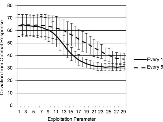
The SLIDER computational model can be used to demonstrate predicted per-formance over a range of Exploitation Parameter values. This is accomplished by setting the model to learn the task, as opposed to fitting human response data. The task is run thousands of times at various levels of Exploitation Parameter. Additionally, two versions of the task were tested: a full feedback scenario (full reward feedback on every trial), versus an intermittent feedback scenario (full reward feedback only every fifth trial, otherwise limited binary feedback).

Figure 1 illustrates that while higher levels of exploitation are generally im-portant for effective learning, intermittent feedback is predicted to be detrimen-tal. Although, the model predicts that this may be overcome by adopting a more exploitative strategy. Based on our model, with regards to performance, in rela-tion to sensitivity to only positive reward feedback (successful trials) versus neg-ative reward feedback (unsuccessful trials), participants should be more sensitive to positive feedback at learning and somewhat more sensitive to negative feed-back at test. Therefore, based on reward feedfeed-back, we would expect differential

effects on performance in the test phase of our experiments, as compared to the learning phase.

2. Experiment 1

2.1. Method

71 participants were recruited from the Queen Mary, University of London community and on average received £5.46 (approx. $9). Fifty-five of the partic-ipants were female, and ages ranged from 18 to 36 (M = 20.02, SD = 3.52). Par-ticipants were randomly assigned to the Gains intermittent condition (n = 26), Losses intermittent condition (n = 25). For the frequent feedback conditions, participants were randomly allocated to Gains frequent condition (n = 10) or the Losses frequent condition (n = 10). The number of participants allocated to the frequent condition was less than that of the intermittent feedback condi-tions, for the following reasons. Considerable prior work (Osman et al., 2015; Osman & Speekenbrink, 2011, 2012) using the same task design has shown that the pattern of responses to frequent feedback in exact same stable dynamic de-cision-making tasks used presently is consistent, particular when participants are exposed to the same length of training trials (i.e. 100 training trials), as is the case with the present set of experiments. Therefore, there was already an established baseline of reliable performance in frequent feedback conditions, which were directly comparable to the conditions designed in our experiments, so for this reason we allocated more participants to the novel conditions de-signed in this Experiment. Moreover, we applied the same rationale to Experi-ment 2 and 3.

2.1.2. Procedure

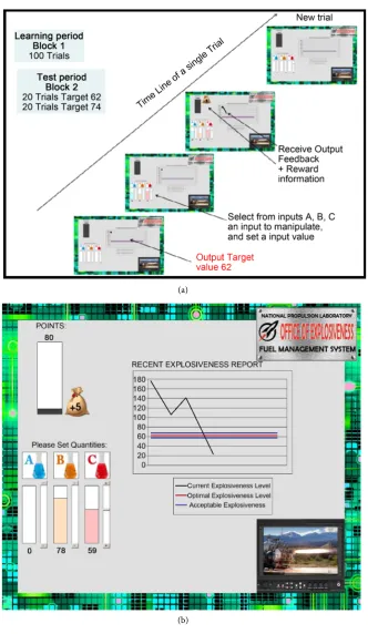
In the present dynamic control task, the participant attempted to control a single output value towards a target goal (see Figure 2). To do so, on each trial the par-ticipant chooses values for three separate inputs. These input values are then combined via the dynamic control equation (Equation (1)) then summed with the output value plus some normally distributed random noise (standard devia-tion = 8). In this way, the participant’s input selecdevia-tions guide the output value. The output value is initialized at 178 with a goal value of 62 and a “safe range” (±10 around the goal value):

( )

(

)

( )

( ) ( )

y t = y t− + x t − x t +e t ₍₅₎ where y(t) is the output on trial t, x1 is the positive input, x2 is the negative input, and e is an error term randomly sampled from a normal distribution with a mean of 0 and SD of 8.

(a)

(b)

the resulting movement of the output value on each trial. After each trial, the input values are reset to 0. The participant can then freely select input values for each of the three inputs before confirming the choices. A critical feature of this control task is that the output value can go below the target, meaning the partic-ipant must dynamically adapt in order to maximize performance. After an initial learning phase of 100 trials (Block 1), the participants completed two Test blocks of 20 trials each. In the first Test block (Block 2), the starting value and goal cri-terion were equivalent to the learning phase. In the second Test block (Block 3), there was a different starting value and goal value than the earlier phases. At the beginning of each block, the control task was reset to the initial state. Partici-pants were able to view a plot of the output value as it changed from trial to trial. In Experiment 1 for infrequent conditions, this plot was available only on every 5 trials. In Block 1, it was available on each of the first 5 trials, thereafter it was only presented every 5th _{trial. For the frequent conditions, this plot was available} only every trial for both Block 1 and Block 2 and Block 3; this was the only criti-cal difference between the manipulation of the frequency of feedback between gains/losses frequent conditions and gains/losses infrequent conditions.

Task performance was incentivized using a point paradigm which was ex-plained to them in advance of taking part in the experiment. Participants at-tempted to either incrementally earn points towards a points criterion (Gains conditions), or prevent losing points to remain above a points criterion (Losses condition). A response which moved the output value towards the goal criterion (relative to the previous trial) was considered a “correct” response, while a re-sponse which moved the output value away from the goal criterion was consi-dered an “incorrect” response. In the Gains condition, participants started with 0 points and achieved +10 points for a correct response, and +5 points for an in-correct response. In the Losses condition, participants started with 1500 (in Block 1, 300 in Blocks 2 and 3) and achieved −5 points for a correct response, and −10 points for an incorrect response. The points criterion was 1500 (Block 1) and 300 (Blocks 2 and 3) for the Gains condition and 0 for the Losses condi-tion.

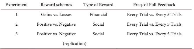
The selection of the values 1500 for Block 1, and 300 for Block 2 and 3, was based on pilot work in which we determined point allocations that would make the Gains and Losses conditions approximately equivalent in terms of available points. Thus, participants were given Gains or Losses information on each trial, despite only being able to view the output value plot (i.e., the Full Feedback In-formation) on every 5th trial (see Table 1).

Table 1. Overview of the experimental design.

Experiment Reward schemes Type of Reward Freq. of Full Feedback 1 Gains vs. Losses Financial Every Trial vs. Every 5 Trials 2 Positive vs. Negative Social Every Trial vs. Every 5 Trials 3 Positive vs. Negative Social Every Trial vs. Every 5 Trials

(replication)

2.2. Results

2.2.1. Deviation from Optimal Response

Post-hoc power analyses for all below experiments resulted in Power ranging from 0.80 to 0.98 (with α = 0.05, and non-centrality parameter λ ranging from 15.0 to 26.6), demonstrated very good statistical power with which to interpret the results. In order to measure task performance, the deviation from the optim-al response was coptim-alculated for each trioptim-al. The optimoptim-al response was coptim-alculated by considering the hypothetical settings for the three input inputs which would have moved the output value as close as possible to the goal criterion. The devia-tion from this response was calculated using the actual participant responses for the three input inputs. For example, if the participant selected values of {50, 60, 40} on the {positive, negative, neutral} input inputs, the previous output value was 90, and the randomly sampled error term was +2, then the new output value would be 90 + 50 − 60 + 2 = 82. The presented magnitude of change would be 8 and the presented direction of change would be toward the goal of 62 (positive reward). In this case, the set of optimal input selections would have varied li-nearly from {0, 18, any} to {82, 100, any}. Thus, the solution with the shortest Euclidean distance to the participant’s choices would have been {46, 64, any}, with a distance of 5.66. This value represents the deviation from optimal re-sponse, and was computed for each trial.

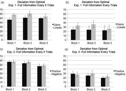
A 2 Feedback Frequency (Every trial, Every 5 trials) × 2 reward schedule (Gains, Losses) × 3 Block (Block 1, Block 2, Block 3) repeated measures ANOVA was conducted on the deviation from optimal response. There was a significant main effect of reward schedule (F1,67 = 5.59, p = 0.02, η2 = 0.08) across both fre-quent and intermittent feedback conditions, such that in general those in the Gains conditions provided more optimal responses relative to Losses conditions. Moreover, there was a strong main effect of Feedback Frequency (F1,67 = 51.7,

p < 0.001, η2 _{= 0.44) such that participants who received frequent feedback} demonstrated more optimal responses than those in the Intermittent feedback conditions (see Figure 3). All other contrasts were non-significant (Fs < 2).

2.2.2. Response Variability during Partial Feedback

Figure 3. Mean output scores (Standard Error ± 1) based on calculation of deviations from optimal by Experiment (Experiment 1, Experiment 2), by reward scheme and type (Experiment 1: Gains vs. Losses; Experiment 2: Negative vs. Positive social feedback).

schedule (Gains, Losses) × 3 Block repeated measures ANOVA on response va-riability. There were no significant main effects or contrasts (all Fs < 1.3; see

Figure 4).

2.2.3. Computational Modeling

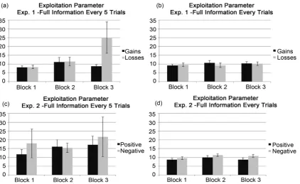
The SLIDER model was used to calculate the best fitting exploitation parameter for each block. In the model, as the Exploitation parameter reaches ∞, the more likely the model is to peak pick the response with the highest estimated expected value. At an Exploitation parameter of 0, the model is equally likely to pick any of the response options (i.e., the response probability distribution is uniform). A 2 Feedback Frequency (Every trial, Every 5 trials) × 2 reward schedule (Gains, Losses) × 3 Block repeated measures ANOVA was conducted on the best fit Ex-ploitation parameter. There were no significant main Effects or contrasts (all Fs < 1.8; see Figure 3) (see Figure 5).

2.3. Discussion

Figure 4. Mean response variability scores (Standard Error ± 1) during trial periods when output value informa-tion was unavailable to the participant, by Experiment (Experiment 1, Experiment 2), by reward scheme and type (Experiment 1: Gains vs. Losses; Experiment 2: Negative vs. Positive social feedback).

Figure 5. Mean (Standard Error ± 1) best fitting exploitation parameters using the SLIDER model, with mean ex-ploitation fits scores based on calculation of deviations from optimal by Experiment (Experiment 1, Experiment 2), by reward scheme and type (Experiment 1: Gains vs. Losses; Experiment 2: Negative vs. Positive social feedback).

Providing full information did not lead to differences in exploitative behavior nor response variability, although there was an overall main effect of gains ver-sus losses framing. Those in the gains condition, regardless of the level of tri-al-by-trial information provided, responded more optimally. This result is in line with the regulatory focus literature which predicts a regulatory match when local incentives match with global incentives. Whether a regulatory match is benefi-cial depends on task demands (Grimm, Markman, Maddox, & Baldwin, 2008). In the present dynamic decision making task, the match of the local and global rewards framework leads to performance enhancements. When feedback is in- termittent, the mismatch condition responds more conservatively (lower re-sponse variability, more exploitative choices), leading to poorer performance. This suggests that dynamic decision making tasks are more compatible with ex-ploratory and flexible choice strategies, and that this is exacerbated when feed-back information is limited.

3. Experiment 2

3.1. Method

In Experiments 1, participants were incentivized with a point goal criterion which incremented on each trial (increasing in Gains, decreasing in Losses) de-pending on performance. In order to test the differential impact of positively versus negatively valenced reward signals, we developed a method which dis-played either feedback in terms of a social reward signal; participants still ceived financial rewards relative to performance, but the presentation of the re-wards was presented socially rather than financially. In both conditions, after each trial, participants were shown an image of their purported supervisor’s re-sponse to their rere-sponse selection. In the Positive condition, the image was ei-ther happy (“correct” trial i.e., closer to target) or neutral (“incorrect” trial i.e., further away from target). In the Negative condition, the image was either neu-tral (correct trial) or negative (incorrect trial; see Figure 6).

Thus, the payoff structure remained the same as in Experiment 1, although the reward presentation was in the form of social feedback. This social feedback indicated trial-by-trial performance and translated into the performance-related bonus payment using the same payment schedule as in the Gains/Losses condi-tions in Experiment 1.

3.1.1. Participants

64 participants were recruited from the Queen Mary, University of London community and paid £6 ($9). 45 of the participants were female, and ages ranged from 18 to 49 (M = 27.4, SD = 5.12). Participants were randomly assigned to the Positive infrequent feedback condition (n = 31) or the Negative infrequent con-dition (n = 31). Both concon-ditions were exposed to the same intermittent output feedback set up. Participants in the frequent feedback conditions were randomly assigned to the Positive frequent feedback condition (n = 11) or the Negative frequent feedback condition (n = 11). All participants were recruited from the Queen Mary, University of London community and on average received £5.52 (approx. $9).

3.1.2. Procedure

Experiment 2 differed from Experiment 1 only in that reward feedback informa-tion was given in the form of either positively or negatively valenced social re-ward information, but output feedback was presented intermittently either every fifth trial in each of the three blocks for the infrequent feedback conditions, or on every trial in the frequent feedback conditions.

3.2. Results

3.2.1. Deviation from Optimal Response

To examine performance, we conducted a 2 Feedback Frequency (Every trial, Every 5 trials) × 2 social reward schedule (Positive, Negative) × 3 Block (Block 1, Block 2, Block 3) repeated measures ANOVA on the deviation from optimal re-sponse. There was a significant main effect of Block (F2,120 = 7.66, p ≤ 0.001, η2 = 0.11) consistent with increasing performance from Block 1 to Block 3 (see Fig-ure 3). Moreover, there was a strong main effect of Feedback Frequency (F1,60 = 52.5, p < 0.001, η2 _{= 0.47) such that participants who received frequent feedback} demonstrated more optimal responses (see Figure 3). All other interactions were non-significant (Fs < 1).

3.2.2. Response Variability during Partial Feedback

To compare response variability during infrequent feedback (every fifth trial) to frequent feedback (every trial), we conducted a 2 Feedback Frequency (Every trial, Every 5 trials) × 2 social reward schedule (Positive, Negative) × 3 Block re-peated measures ANOVA on the variability of response variability. There were no significant main Effects or interactions (all Fs < 1.5; see Figure 4).

3.2.3. Computational Modeling

(Positive, Negative) × 3 Block repeated measures ANOVA was conducted on the best fit Exploitation parameter. There were no significant main effects or inte-ractions (all Fs < 3.4; see Figure 5).

3.3. Discussion

In Experiment 1, the Gains condition demonstrated more optimal performance relative to the Losses condition over both full and infrequent feedback condi-tions. In Experiment 2, we did not detect a performance difference between pos-itive and negative social reward conditions. Consistent with Experiment 1, those in the frequent feedback conditions demonstrated enhanced performance rela-tive to those with infrequent feedback. As expected, this contrast demonstrates that people are able to use the trial-by-trial information to inform their decisions on this dynamic decision making task. Interestingly, performance in Experiment 2 increased over blocks, whereas this performance increase was not detected in Experiment 1. Post-hoc analysis suggests that this difference was due to stable yet more optimal performance by the Gains condition in Experiment 1, as well as shifts in strategy over time by the Losses condition in Experiment 1 as meas-ured by response variability and best fit exploitation parameter. The perfor-mance increase over time detected in Experiment 2 could be the result of de-creased sensitivity to the social reward feedback manipulation, which lead to fewer shifts in strategy and the emergence of a general learning curve. The lack of a local and global rewards framing effect when local rewards were operationa-lized as social reward indicates that either our social reward stimuli were ineffec-tive in eliciting the necessary response, or the results support previous findings that social and monetary rewards are processed by different underlying neural structures. Rademacher et al. (2010) provides evidence that while anticipation for both monetary and social rewards activate brain areas important for learn-ing, social stimuli was more strongly associated with amygdala activation, while monetary stimuli were more associated with thalamic activation. While mone-tary activation was also part of the global rewards framing in Experiment 2, along with social reward, it is possible that overall increased activation in Expe-riment 2 minimized differences between the positive and negative social re-wards. To establish the reliability of the findings in Experiment 2, we replicated them in Experiment 3.

4. Experiment 3

4.1. Method

4.1.2. Procedure

Experiment 3 was a replication of Experiment 2, and did not differ from them. In one condition, value information was presented on each trial, and in another condition it was presented on every 5 trials. The Positive and Negative social re-ward schedules were implemented identically to Experiment 2.

4.2. Results

4.2.1. Deviation from Optimal Response

As Experiment 3 was conducted as a replication of Experiment 2, we conducted a 2 Feedback Frequency (Every trial, Every 5 trials) × 2 social reward schedule (Positive, Negative) × 3 Block repeated measures ANOVA on the deviation from optimal response. There was a strong main effect of Feedback Frequency (F1,36 = 49.17, p < 0.001, η2 _{= 0.58) such that participants who received full information} feedback on each trial demonstrated more optimal responses. All other interac-tions were non-significant (Fs < 3.2).

4.2.2. Response Variability during Partial Feedback

To compare response variability during infrequent (every fifth trial) to frequent (every trial), we conducted a 2 Feedback Frequency (Every trial, Every 5 trials) × 2 social reward schedule (Positive, Negative) × 3 Block repeated measures ANOVA on the variability of response variability. There were no significant main Effects or interactions (all Fs < 2.5).

4.2.3. Computational Modeling

A 2 Feedback Frequency (Every trial, Every 5 trials) × 2 social reward schedule (Positive, Negative) × 3 Block repeated measures ANOVA was conducted on the best fit Exploitation parameter. There were no significant main effects or inte-ractions (all Fs < 3.1).

4.3. Discussion

Experiment 3 was a replication of Experiment 2 in that frequency of feedback (Every trial vs. Every 5 trials) and social reward valence (Positive vs. Negative) were manipulated as between subjects factors, repeated over 3 Blocks of trials. In Experiment 3, there was a main effect of Feedback Frequency, in that those who received full information regarding the output value on each trial responded more optimally than those who received full information on every 5th trial. Taken together, the results from Experiments 2 & 3 signify that full feedback frequency is important for optimal decision making in dynamic decision making environments with multiple inputs with a hidden but discoverable relationship to the output variable. However, we did not detect a difference in performance between those who received information via a positively valenced social reward channel versus a negatively valenced social reward channel.

5. General Discussion

(out-put feedback) is presented infrequently or frequently. Overall our key experi-mental manipulations impacted behavior when reward signals were presented as money, and the impact of intermittent feedback on performance was limited to reducing optimality performance. The remainder of the discussion will consider the implications of our findings with respect to frequency of presentation of output feedback, the impact of rewards on dynamic decision-making, and com-putational models of dynamic decision-making.

5.1. Frequent vs. Intermittent Feedback

Overall, our findings contrast work looking at the effects of intermittent feed-back on forecasting (Frederickson et al., 1999; Lurie & Swaminathan, 2009)

which suggests frequent output feedback results in poorer judgment accuracy. One key difference between this work and the present study is that we set up the experiments in such a way that participants were encouraged to go beyond a fully exploitative strategy because during the trials in which no output feedback was presented, there was always trial-by-trial partial feedback via reward infor-mation that provided directional inforinfor-mation (the sign but not the precise mag-nitude of the change to the output). This is why we also speculated that output feedback presented on every trial would lead to better performance than infre-quent output feedback, because in the latter case, the most rich information on which to learn was presented 20% of the time as compared to 100% of the time in the frequent feedback set-ups. However, in general participants seemed to keep to the same strategy regardless of whether they were waiting for the next update of output information every fifth trial, or on every trial. This suggests that the nature of the task itself is one that might induce a consistent application of a strategy once one has been found. In line with this, previous work (Osman & Speekenbrink, 2011) reported that regardless of how stable or extremely unst-able the dynamic environment was, strategic behavior tended to be consistent, to the extent that participants perseverated even when the visual display on screen clearly indicated how poor their chosen strategy was doing. Furthermore, many studies have shown that participants in dynamic decision-making tasks tend to be rather conservative with respect to adjusting their strategies once they have settled on them (Burns & Vollmeyer, 2002; Osman, 2008a, 2008b, 2012; Voll-meyer et al, 1996). This suggests that, as a result of a high state of uncertainty experienced in such tasks (Lipshitz & Strauss, 1997;Sterman, 1989), people are reluctant to give up current strategies once they have been established. This leads to an over-commitment to a strategy regardless of the frequency of the feedback.

5.2. Financial vs. Social Rewards

as in the social rewards framing, they had to translate the reactions of the man-ager into gains or losses and then convert this into monetary gains and losses to figure out how much they would get at the end of the experiment. Therefore, one simple explanation is that it isn’t the fact that rewards presented as financial gains and losses per se that led to the difference between social and financial signals, but simply the fact that the financial signals were easier to interpret as reward signals because no conversion was needed.

A second possible explanation is that social reward signals are more ambi-guous or more complex, and carry different meanings for different individuals, and this in turn leads to the signals being perceived in different ways, which in-creases the variability in decision-making behavior. There is a growing trend in the finance literature to examine the effects of financial rewards on social beha-vior (Aktas, De Bodt, & Cousin, 2011;Camerer & Ho, 1999;Margolis, Elfenbein, & Walsh, 2007; Oikonomou, Brooks, & Pavelin, 2014). Overall, the findings from these studies suggest that the impact of social rewards vs. financial rewards on behavior depends largely on the context in which the behavior is examined. In particular, social rewards improve status or reputation are effective in moti-vating and improving performance but only in contexts in which these factors are relevant and appreciated by a norm. For future work, it may be the case that activating social norms in the form of social rewards represented by a group would lead to better dynamic decision-making performance than simply pre-senting social rewards connected to a single participant (Andersson, He-desström, & Gärling, 2014).

In general, the most consistent findings regarding reward information was that a reward schedule that only involved rewards tied to performance was more effective in improving performance relative to a loss only reward schedule. We speculate that one likely reason for the differences between the two framings is the differential impact they have on the decision-makers’ confidence. Consistent with this speculation, work looking at the association between rewards and be-havior has often reported that people see rewards as potential reinforces of self-esteem, which can in turn boost performance (Bushman, Moeller, & Crock-er, 2011). Also, there is work suggesting that rewards may induce confidence or even over confidence which can negatively impact performance (González-Val- lejo, & Bonham, 2007; Rudski, Lischner, & Albert, 2012). In addition, there is work showing that rather than positive reinforcement motivating behavior and improving performance, negative reinforcers are a more effective way of im-proving performance. This is either because losses are more psychologically sa-lient than gains (Erev & Barron, 2005;Hossain & List, 2012), or because a nega-tive reinforcer is more informationally useful than a posinega-tive reinforcer because it focuses attention more acutely on the task at hand (Yechiam & Hochman, 2014). One reason for this is that there may be mismatches between the task and the motivation of the individual, which originates from Higgins (1997) regula-tory fit framework.

environments people must trade off the amount of time they want to spend fo-cusing on exploiting, against exploring, in the hope that they will be in a better more rewarding position in the future. When there is a match between one’s motivational state (for which we use instructed goals as a proxy to establish this in the present study) and the reward structure of the task (i.e., regulatory fit), then this determines the extent of exploitation over exploration (Worthy et al., 2007). Broadly our findings were supportive of the regulatory fit position. Those in the gains conditions showed more exploration because there was a fit between the global and local reward structures, regardless of the fact that this was a sub-optimal learning strategy (a finding similar to that reported by Worthy et al. (2007, Exp 2). Curiously though, in our study, those in the gains condition also out performed those in the losses condition, despite using a sub-optimal learn-ing strategy, even though it was matched to the global strategy. One reason for this is that there are multiple layers of strategies that constitute a fit and a mis-match in our present dynamic decision-making task, and it may be the case that matches on some levels are more important for enabling good control perfor-mance over others. For instance, a decision-maker in a dynamic decision-mak- ing task may view their strategy of attempting to reach the target criterion on each trial as a promotion focused strategy. Another decision-maker may view their attempt to maintain the target criterion for the remaining length of the training/test trials after having reached it as a prevention focused strategy. While the regulatory fit theory predicted the type of learning strategy that was imple-mented, this in turn does no necessary predict the success of control perfor-mance in our decision-making task.

5.3. Computation Models

in the use of increased exploitative choice patterns. In Experiment 1, under fi-nancial rewards, those under intermittent feedback and a losses reward structure do show evidence of utilizing a strategy of increased exploitation in order to achieve matched performance. The computational modeling approach outlined here demonstrates that it is possible to capture and describe compensatory me-chanisms under regulatory mismatch in terms of differences in associative learning along the exploration-exploitation dimension.

5.4. Implications and Applications beyond the Dynamic

Decision-Making Literature

Characterizing unstable dynamic environments, measuring the impact of dif-ferent policies and regulations on behavior within them, and understanding what the factors are that cause instability in order to minimize it, seem to be central issues for many researchers in the management, accounting, banking and finance disciplines (Aktas et al., 2011;Bandiera et al., 2011;Margolis et al., 2007; Melancon et al., 2011;Melnyk, Bititci, Platts, Tobias, & Andersen, 2014; Oiko-nomou et al., 2014). These issues lend themselves to paradigms such as dynamic control tasks which essentially are toy complex worlds that enable researchers to explore multiple factors in the lab (Meder, Le Lec, & Osman, 2013). We show, according to our conceptualization of optimality, the extent to which people be-have optimally, and the factors that enhance (positive reinforcement, frequently presented output feedback) optimal dynamic decision-making. Critically, we al-so show that it is possible to incorporate incentive schemes in such a way as to connect them to performance, so that they are meaningful. Our findings reveal that financially framed rewards are more potent than socially framed rewards, and that only in the former do they induce differences in decision-making and learning behaviors (response variability, exploration). These insights can poten-tially offer same basic understanding of human behavior in dynamic environ-ments in order to pave the way to answering big practical questions such as: What are the appropriate frameworks for assessing the effects of reforms aimed at mitigating financial stability? What is the most effective way of ensuring that regulation addresses dynamically evolving risks to financial stability (Bank of England, 2015)?

References

Aktas, N., De Bodt, E., & Cousin, J.-G. (2011). Do Financial Markets Care about SRI? Evidence from Mergers and Acquisitions. Journal of Banking & Finance, 35, 1753- 1761.

Andersson, M., Hedesström, M., & Gärling, T. (2014). A Social-Psychological Perspective on Herding in Stock Markets. Journal of Behavioral Finance, 15, 226-234.

https://doi.org/10.1080/15427560.2014.941062

Ariely, D., Gneezy, U., Loewenstein, G., & Mazar, N. (2009). Large Stakes and Big Mis-takes. The Review of Economic Studies, 76, 451-469.

https://doi.org/10.1111/j.1467-937X.2009.00534.x

Experimental Psychology, 47, 170. https://doi.org/10.1037/h0053619

Bandiera, O., Barankay, I., & Rasul, I. (2011). Field Experiments with Firms. The Journal of Economic Perspectives, 63-82. https://doi.org/10.1257/jep.25.3.63

Bank of England (2015). One Bank Research Agenda: Discussion Paper.

Bonner, S. E., & Sprinkle, G. B. (2002). The Effects of Monetary Incentives on Effort and Task Performance: Theories, Evidence, and a Framework for Research. Accounting, Organizations and Society, 27, 303-345.

Brehmer, B. (1992). Dynamic Decision Making: Human Control of Complex Systems. Actapsychologica, 81, 211-241.

Brooks, J. D., Wilson, N., & Sun, R. (2012). The Effects of Performance Motivation: A Computational Exploration of a Dynamic Decision Making Task. In Proceedings of the First International Conference on Brain-Mind (pp. 7-14).

Buchheit, S., Dalton, D., Downen, T., & Pippin, S. (2012). Outcome Feedback, Incentives, and Performance: Evidence from a Relatively Complex Forecasting Task. Behavioral Research in Accounting, 24, 1-20. https://doi.org/10.2308/bria-50151

Burns, B. D. & Vollmeyer, R. (2002). Goal Specificity Effects on Hypothesis Testing in Problem Solving. The Quarterly Journal of Experimental Psychology: Section A, 55, 241-261. https://doi.org/10.1080/02724980143000262

Bushman, B. J., Moeller, S. J., & Crocker, J. (2011). Sweets, Sex, or Self-Esteem? Compar-ing the Value of Self-Esteem Boosts with Other Pleasant Rewards. Journal of personal-ity, 79, 993-1012.https://doi.org/10.1111/j.1467-6494.2011.00712.x

Camerer, C. & Ho, T.-H. (1999). Experienced-Weighted Attraction Learning in Normal Form games. Econometrica, 827-874.

https://doi.org/10.1111/1468-0262.00054

Chase, H. W., Kumar, P., Eickhoff, S. B., & Dombrovski, A. Y. (2015). Reinforcement Learning Models and Their Neural Correlates: An Activation Likelihood Estimation Meta-Analysis. Cognitive, Affective & Behavioral Neuroscience, 15, 435- 459.

https://doi.org/10.3758/s13415-015-0338-7

Cisek, P. (2006). Integrated Neural Processes for Defining Potential Actions and decIding between Them: A Computational Model. The Journal of Neuroscience, 26, 9761-9770.

https://doi.org/10.1523/JNEUROSCI.5605-05.2006

Daw, N. D., & Doya, K. (2006). The Computational Neurobiology of Learning and Re-ward. Current Opinion in Neurobiology, 16, 199-204.

Deci, E. L. (1976). Notes on the Theory and Metatheory of Intrinsic Motivation. Organi-zational Behavior and Human Performance, 15, 130-145.

Deci, E. L., & Ryan, R. M. (1985). Intrinsic Motivation and Self-Determination in Human Behavior. Berlin: Springer Science & Business Media.

https://doi.org/10.1007/978-1-4899-2271-7

Eisenberger, R., & Cameron, J. (1996). Detrimental Effects of Reward: Reality or Myth? American Psychologist, 51, 1153.

https://doi.org/10.1037/0003-066X.51.11.1153

Erev, I., & Barron, G. (2005). On Adaptation, Maximization, and Reinforcement Learning among Cognitive Strategies. Psychological Review, 112, 912.

https://doi.org/10.1037/0033-295X.112.4.912

Erev, I., & Roth, A. E. (1998). Predicting How People Play Games: Reinforcement Learn-ing in Experimental Games with Unique, Mixed Strategy Equilibria. American Eco-nomicReview, 848-881.

Environ-ments. Management Science, 59, 573-591.

https://doi.org/10.1287/mnsc.1120.1612

Frederickson, J. R., Peffer, S. A., & Pratt, J. (1999). Performance Evaluation Judgments: Effects of Prior Experience under Different Performance Evaluation Schemes and Feedback Frequencies. Journal of Accounting Research, 151-165.

https://doi.org/10.2307/2491401

Frey, B. (1997). Not Just for the Money: An Economic Theory of Personal Motivation. Cheltenham: Elgar.

Gibson, F. P. (2007). Learning and Transfer in Dynamic Decision Environments. Com-putational and Mathematical Organization Theory, 13, 39-61.

https://doi.org/10.1007/s10588-006-9010-7

González-Vallejo, C., & Bonham, A. (2007). Aligning Confidence with Accuracy: Revisit-ing the Role of Feedback. Acta Psychologica, 125, 221-239.

Grimm, L. R., Markman, A. B., Maddox, W. T., & Baldwin, G. C. (2008). Differential Ef-fects of Regulatory fit on Category Learning. Journal of Experimental Social Psycholo-gy, 44, 920-927.

Hertwig, R., & Ortmann, A. (2001). Experimental Practices in Economics: A Methodo-logical Challenge for Psychologists? Behavioral and Brain Sciences, 24, 383- 403.

https://doi.org/10.2139/ssrn.1129845

Higgins, E. T. (1997). Beyond Pleasure and Pain. American Psychologist, 52, 1280.

https://doi.org/10.1037/0003-066x.52.12.1280

Hossain, T., & List, J. A. (2012). The Behavioralist Visits the Factory: Increasing Produc-tivity Using Simple Framing Manipulations. Management Science, 58, 2151- 2167.

https://doi.org/10.1037/0003-066X.52.12.1280

Kamenica, E. (2012). Behavioral Economics and Psychology of Incentives. Annual Review of Economics, 4, 427-452.

https://doi.org/10.1146/annurev-economics-080511-110909

Le Pelley, M. E. (2004). The Role of Associative History in Models of Associative Learn-ing: A Selective Review and a Hybrid Model. Quarterly Journal of Experimental Psy-chologySection B, 57, 193-243.

https://doi.org/10.1080/02724990344000141

Lepper, M. R., & Greene, D. (2015). The Hidden Costs of Reward: New Perspectives on the Psychology of Human Motivation. London: Psychology Press.

Lipshitz, R., & Strauss, O. (1997). Coping with Uncertainty: A Naturalistic Decision- Making Analysis. Organizational Behavior and Human Decision Processes, 69, 149- 163. https://doi.org/10.1006/obhd.1997.2679

Luckett, P. F., & Eggleton, I. R. (1991). Feedback and Management Accounting: A Review of Research into Behavioral Consequences. Accounting, Organizations and Society, 16, 371-394.

Lurie, N. H., & Swaminathan, J. M. (2009). Is Timely Information Always Better? The Ef-fect of Feedback Frequency on Decision Making. Organizational Behavior and Human Decision Processes, 108, 315-329.

Luce, R. D. (1959). On the Possible Psychophysical Laws. Psychological Review, 66, 81-95.

https://doi.org/10.1037/h0043178

Margolis, J. D., Elfenbein, H. A., & Walsh, J. P. (2007). Does It Pay to Be Good? A Me-ta-Analysis and Redirection of Research on the Relationship between Corporate Social and Financial Performance. Ann Arbor, 1001, 48109-1234.

https://doi.org/10.2139/ssrn.1866371

Review and a Prediction Model. In M. Lepper, & D. Greene (Eds.), The Hidden Costs of Reward: New Perspectives on the Psychology of Human Motivation (pp. 33-60). London: Psychology Press.

Meder, B., Le Lec, F., & Osman, M. (2013). Decision Making in Uncertain Times: What Can Cognitive and Decision Sciences Say about or Learn from Economic Crises? Trends inCognitive Sciences, 17, 257-260.

Melancon, J. P., Noble, S. M., & Noble, C. H. (2011). Managing Rewards to Enhance Re-lational Worth. Journal of the Academy of Marketing Science, 39, 341-362.

https://doi.org/10.1007/s11747-010-0206-5

Melnyk, S. A., Bititci, U., Platts, K., Tobias, J., & Andersen, B. (2014). Is Performance Measurement and Management Fit for the Future? Management Accounting Research, 25, 173-186.

Oikonomou, I., Brooks, C., & Pavelin, S. (2014). The Effects of Corporate Social Perfor-mance on the Cost of Corporate Debt and Credit Ratings. Financial Review, 49, 49-75.

https://doi.org/10.1111/fire.12025

Osman, M. (2008a). Observation Can Be as Effective as Action in Problem Solving. Cog-nitiveScience, 32, 162-183. https://doi.org/10.1080/03640210701703683

Osman, M. (2008b). Positive Transfer and Negative Transfer/Antilearning of Prob-lem-Solving Skills. Journal of Experimental Psychology: General, 137, 97.

https://doi.org/10.1037/0096-3445.137.1.97

Osman, M. (2010). Controlling Uncertainty: A Review of Human Behavior in Complex Dynamic Environments. Psychological Bulletin, 136, 65.

https://doi.org/10.1037/a0017815

Osman, M. (2012). The Effects of Self Set or Externally Set Goals on Learning in an Un-certain Environment. Learning and Individual Differences, 22, 575-584.

Osman, M. (2014). Future-Minded: The Psychology of Agency and Control. Palgrave Macmillan.https://doi.org/10.1007/978-1-137-02227-1

Osman, M., Glass, B. D., & Hola, Z. (2015). Approaches to Learning to Control Dynamic Uncertainty. Systems, 3, 211-236. https://doi.org/10.3390/systems3040211

Osman, M., & Speekenbrink, M. (2011). Cue Utilization and Strategy Application in Sta-ble and UnstaSta-ble Dynamic Environments. Cognitive Systems Research, 12, 355-364. Osman, M., & Speekenbrink, M. (2012). Prediction and Control in a Dynamic

Environ-ment. Frontiers in Psychology, 3. https://doi.org/10.3389/fpsyg.2012.00068

Otto, A. R., Markman, A. B., Gureckis, T. M., & Love, B. C. (2010). Regulatory Fit and Systematic Exploration in a Dynamic Decision-Making Environment. Journal of Expe-rimental Psychology: Learning, Memory, and Cognition, 36, 797.

https://doi.org/10.1037/a0018999

Rademacher, L., Krach, S., Kohls, G., Irmak, A., Gründer, G., & Spreckelmeyer, K. N. (2010). Dissociation of Neural Networks for Anticipation and Consumption of Mone-tary and Social Rewards. Neuroimage, 49, 3276-3285.

Rudski, J. M., Lischner, M. I., & Albert, L. M. (2012). Superstitious Rule Generation Is Affected by Probability and Type of Outcome. Psychological Record, 49, 245-260. Smith, V. L., & Walker, J. M. (1993). Monetary Rewards and Decision Cost in

Experi-mental Economics. Economic Inquiry, 31, 245-261.

https://doi.org/10.1111/j.1465-7295.1993.tb00881.x

Sterman, J. D. (1989). Modeling Managerial Behavior: Misperceptions of Feedback in a Dynamic Decision Making Experiment. Management Science, 35, 321-339.

Sun, R., Slusarz, P., & Terry, C. (2005). The Interaction of the Explicit and the Implicit in Skill Learning: A Dual-Process Approach. Psychological Review, 112, 159.

https://doi.org/10.1037/0033-295X.112.1.159

Sutton, R. S., & Barto, A. G. (1998). Reinforcement Learning: An Introduction. Cam-bridge: MIT Press.https://doi.org/10.1109/tnn.1998.712192

Van Pham, H., Tran, K. D., & Kamei, K. (2014). Applications Using Hybrid Intelligent Decision Support Systems for Selection of Alternatives under Uncertainty and Risk. International Journal of Innovative Computing, Information and Control, 10, 39-56. Vera-Munoz, S. C. (1998). The Effects of Accounting Knowledge and Context on the

Omission of Opportunity Costs in Resource Allocation Decisions. Accounting Review, 47-72.

Vollmeyer, R., Burns, B. D., & Holyoak, K. J. (1996). The Impact of Goal Specificity on Strategy Use and the Acquisition of Problem Structure. Cognitive Science, 20, 75-100.

https://doi.org/10.1207/s15516709cog2001_3

Worthy, D. A., Maddox, W. T., & Markman, A. B. (2007). Regulatory Fit Effects in a Choice Task. Psychonomic Bulletin & Review, 14, 1125-1132.

https://doi.org/10.3758/BF03193101

Yechiam, E., Busemeyer, J. R., Stout, J. C., & Bechara, A. (2005). Using Cognitive Models to Map Relations between Neuropsychological Disorders and Human Decision-Mak- ing Deficits. Psychological Science, 16, 973-978.

https://doi.org/10.1111/j.1467-9280.2005.01646.x

Yechiam, E., & Hochman, G. (2014). Loss Attention in a Dual-Task Setting. Psychological Science, 25, 494-502. https://doi.org/10.1177/0956797613510725

Submit or recommend next manuscript to SCIRP and we will provide best service for you:

Accepting pre-submission inquiries through Email, Facebook, LinkedIn, Twitter, etc. A wide selection of journals (inclusive of 9 subjects, more than 200 journals)

Providing 24-hour high-quality service User-friendly online submission system Fair and swift peer-review system

Efficient typesetting and proofreading procedure

Display of the result of downloads and visits, as well as the number of cited articles Maximum dissemination of your research work

Submit your manuscript at: http://papersubmission.scirp.org/