Munich Personal RePEc Archive
Experimental Evidence on Valuation and
Learning with Multiple Priors
Qiu, Jianying and Weitzel, Utz
Radboud University Nijmegen, Institute for Management Research,
Department of Economics,
24 January 2013
Online at
https://mpra.ub.uni-muenchen.de/43974/
Experimental evidence on valuation and learning with
multiple priors
Jianying Qiu∗ Utz Weitzel†‡
January 24, 2013
Abstract
Popular models for decision making under ambiguity assume that people use not
one but multiple priors. This paper is a first attempt to experimentally elicit multiple
priors. In an ambiguous scenario with two underlying states we measure a subject’s
single prior, her other potential priors (multiple priors), her confidence in these priors
valuation of an ambiguous asset with the same underlying states. We also investigate
subjects’ updating of (multiple) priors after receiving signals about the true states. We
find that single priors are best understood as a confidence-weighted average of
mul-tiple priors. Single priors also predict the valuation of ambiguous assets best, while
both the minimum and maximum of subjects’ multiple priors add explanatory power.
This provides some but no exclusive support for the maxmin (Gilboa and Schmeidler,
1989) and the αmaxmin model (Ghirardato et al., 2004). With regard to updating
of priors, we do not observe strong deviations from Bayesian learning, although
sub-jects overadjust/underadjust their priors and their confidence in multiple priors after
a contradictory/confirming signal. Subjects also react to neutral information with
∗Radboud University Nijmegen, Institute for Management Research, Department of Economics, Thomas
van Aquinostraat 5, 6525GD Nijmegen, The Netherlands
†Radboud University Nijmegen, Institute for Management Research, Department of Economics, Thomas
van Aquinostraat 5, 6525GD Nijmegen, The Netherlands
Ru-more confidence in their priors. This holds under ambiguity, but not in a comparison
treatment under risk.
Keywords: ambiguity, uncertainty, risk, multiple priors, Bayesian updating,
first-order beliefs, second-first-order beliefs
1
Introduction
In many real-world situations there is too little information to form an unique prior that
individuals feel confident enough to use as a sole base for decision making. In such
sit-uations of ambiguity, people may not only have one but multiple priors, which they use
in their decision making process. The maxmin model (Gilboa and Schmeidler, 1989), α
maxmin model (Ghirardato et al., 2004), and the smooth models of ambiguity (Klibanoff
et al., 2005; Nau, 2006) explicitly consider multiple priors and they are probably the most
popular models used to explain the valuation of assets under ambiguity. Although
perti-nent literature tested the predictions of multiple prior models (e.g., Hey et al., 2010), there
is no study, to the best of our knowledge, that elicits and characterizes multiple priors.
Moreover, there is no theory or direct evidence on the updating process of multiple priors
under ambiguity. This paper therefore is a first attempt to measure beliefs with multiple
priors and their updating under ambiguity.
Characterizing beliefs under ambiguity when it is possible to have multiple priors is tricky.
It calls for higher orders of beliefs. Consider, for example, an ambiguous Ellsberg urn
(Ellsberg, 1961) with ten balls that are either white or black. Since a prior is a belief system
that completely describes an individual’s subjective beliefs of the ambiguous scenario,
we would need ten first-order subjective beliefs, with each belief corresponding to the
individual’s likelihood estimation of one of the ten potential underlying states. That is,
ten first-order subjective beliefs constitute one prior. If we want to study beliefs involving
multiple priors, we need to elicit second-order beliefs: an individual’s confidence in all
potential priors.1 Such a procedure can be very complicate and counter-intuitive. It is
1
difficult enough to properly elicit one prior. To elicit more than one prior from the same
individual appears to be impossible. Even if such a procedure could be implemented, it
would be difficult to find an incentive compatible mechanism for it, which may be the
reason why multiple priors have never been empirically elicited so far.2
To measure beliefs with multiple priors we construct an ambiguous scenario with two
potential states of world. With binary outcomes, a single first-order subjective belief
regarding either state of the world completely describes an individual’s probability measure
of all states of the world, and hence is a prior of the individual. To examine an experimental
participant’s multiple priors, we ask each participant to state her confidence in all other experimental participants’ priorsvia an incentive compatible mechanism. That is, we elicit a probability distribution for priors. As the confidence statement relates to a participant’s
uncertainty of others’ priors it indirectly represents her own perception of uncertainty in
the ambiguous scenario. When guessing the priors of other experimental participants in
the absence of any additional information, subjects arguably use their own perception of
uncertainty.3 For example, in a risky scenario, when there is no ambiguity, we would
assume that expected utility maximizers have a degenerated probability distribution with
a 100 percent confidence in the probability of the risky scenario. It is in this sense that
subjects’ individual confidence distributions relate to multiple priors.
Additionally, we provide experimental participants with signals about the true state of the
ambiguous scenario. This allows us to investigate how individuals update their priors and
multiple priors in reaction to the signals. W use the standard deviation of the confidence
distribution of multiple priors as a proxy of individuals’ perception of uncertainty in the
ambiguous scenario. Individuals with larger standard deviations are less confident in their
prior and may exhibit a different update pattern than individuals with higher confidence
urn with ten black or white balls, a first-order belief normally refers to the overall (expected) probability of a drawn ball being white or black. A second-order belief would then be the ten probabilities for ten potential states of world. Thus, our first-order beliefs correspond to those second-order beliefs, and our second-order beliefs are best interpreted as third-order beliefs.
2
in their priors. As we are able to observe a belief updating path for each individual,
with regard to both her prior and multiple priors, we can directly examine learning in
ambiguous scenarios.
The paper’s two main aspects, the measurement of (i) multiple priors and (ii) belief
up-dating, each contribute to several strands of the literature on ambiguity:
(i) The paper complements the literature that tests various models of ambiguity by
de-veloping and analyzing competing predictions that discriminate between the different
ap-proaches (see, e.g., Hey et al., 2010). By eliciting multiple priors, we are able to test the maxmin model, theα maxmin model, and the smooth ambiguity model (Klibanoff et al., 2005; Nau, 2006) directly. We found that the valuation of ambiguous assets is best
ex-plained by subjects’ single priors, while the mins and the max’s of subjects’ multiple priors
also add explanatory power. This provides some, but no exclusive support for the maxmin
and theαmaxmin model. When comparing the maxmin model and theαmaxmin model, the data gives more support to the latter. Subjects consider both the max and the min
of multiple priors, although they seem to place some more weight on the minimum. In
contrast to intuition, subjects’ overall confidence in their multiple priors (proxied by the
standard deviations of the confidence distributions) do not play an important role in the
evaluation process.
Multiple prior models do not explain how multiple priors collapse into a single prior if
subjects are only allowed to state the latter. In modelling the evaluation of an ambiguous
asset, multiple priors enter the valuation decision directly and without prior aggregation
(Gilboa and Schmeidler, 1989; Ghirardato et al., 2004). In our experiment, however, we
elicit both multiple priors and a single prior that represents an aggregation of the former.
Although it is intuitive to assume that the aggregation of multiple priors into a single prior
is analoguous to the way how multiple priors enter an asset valuation, there is no theory
for this. On a more exploratory note this paper therefore also addresses the relationship
between a subject’s single prior (the prior that a subject reports when she is allowed to
state only one) and her multiple priors. Specifically, we investigate whether the single
most confident in, or a confidence weighted prior. We found that single priors are best
understood as a confidence-weighted average of multiple priors.
(ii) The paper also contributes to the literature on learning under ambiguity. Marinacci
(2002) shows that when an individual can sample with replacement from an ambiguous
scenario, she will learn more and more about the true state. Epstein and Schneider (2007)
demonstrate that learning can eventually resolve ambiguity, in the sense of a shrinking
set of priors. The question remainshow people learn in ambiguous situations. Bossaerts et al. (2010) assume a Bayesian learning process and a number of studies in neuroscience
point into the same direction (Friston, 2003, 2005; Doya et al., 2007, for a comprehensive
overview). But this is not a given. In the light of alternative processes (e.g.
reinforce-ment learning) it is still unclear how people adjust their beliefs when they receive signals
about an ambiguous situation. This paper therefore attempts to shed first light on the
updating process with multiple priors. In general we did not observe strong deviations
from Bayesian learning. This is true both for the updating of single priors and the
up-dating of whole confidence distributions. Interestingly, we found that neutral information
reduced perceived uncertainty in the sense of decreasing standard deviations of confidence
distributions of multiple priors. This result holds in ambiguous scenarios, but not under
risk.
Recent studies on amplification effects suggest that the volatility of stock prices in financial
markets might be related to updating under ambiguity (Illeditsch, 2011; Routledge and
Zin, 2009; Guidolin and Rinaldi, 2010). In particular, there have been speculations that
individuals may update differently when receiving a confirming signal (a signal that is
identical to the previous signal) or a contradictory signal (a signal that is opposed to
the previous signal). This relates to studies that find asymmetric reactions to good or
bad news under ambiguity (Epstein and Schneider, 2008; Illeditsch, 2011; Epstein et al.,
2010). In this paper, we directly test and, more importantly, analyze the learning and
updating process of multiple priors that may underly these features. We found that
subjects overadjusted their beliefs when receiving a contradictory signal and underadjusted
than to good news.
The rest of this paper is organized as follows. Section 2 presents the experimental design.
Section 3 reports and discusses the experimental results and Section 4 concludes.
2
Experimental framework
2.1 Construction of the ambiguous scenario
Although the procedure of the construction of the ambiguous scenario should be
trans-parent, the scenario itself must be sufficiently ambiguous. We therefore implemented the
following procedure.
At the beginning of the experimental session, before the instructions were distributed, each
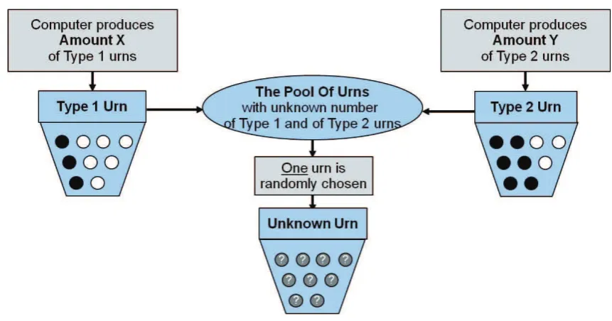
subject was asked to enter 5 pairs of numbers,N1 and N2, into the computer. Subjects only knew that these ten numbers could be any numbers between 0 and 1 million. We
randomly selected one numbern1 out of allN1s and one number n2 out of allN2s. The computer then constructed a pool of urns, which were either of Type 1: 3 black balls and
6 white balls, or of Type 2: 6 black balls and 3 white balls. The total number of Type 1
urns was determined by the chosenn1. The total number of Type 2 urn was determined by the chosen n2. That is, we had n1 urns of Type 1 andn2 urns of Type 2, where n1 andn2 were the same for all participants. Figure 1 provides a screen shot illustrating the construction of the ambiguous scenario.
We randomly selected a single urn from this pool of urns. Note that there are two mutually
exclusive statesS ={S1, S2}of the world in this scenario: S1= The selected urn is of Type 1
and S2 = The selected urn is of Type 2. We asked subjects to estimate the probability
that the underlying state isS1 (the selected urn is of Type 1). As it is very difficult, if
not entirely impossible, to assign objective probabilities to either state of world, subjects
Figure 1: Screen shot illustrating the construction of the ambiguous scenario.
2.2 Elicitation of single priors
Letp denote the probability that the underlying state isS1. Note that, as there are only
two states of world, each subject’s unique prior is completely described by p. We mainly relied on a quadratic scoring rule (hereafter QSR) to elicit priors (Brier, 1950). More
explicitly, subjects were each endowed with 100 points which they could assign to two
alternatives:
Alternative 1: The urn is of Type 1 (with 3 black balls and 6 white balls)
Alternative 2: The urn is of Type 2 (with 6 black balls and 3 white balls)
Letm1 andm2 denote the points that subjects assigned to Alternative 1 and Alternative 2, respectively. Such an assignment of points corresponds to the following payment:
It can be shown that subjects’ expected value is maximized when they choose m1100 and 100m2
to be equal to their respective subjective beliefs. Therefore, m1100 and 100m2 can be taken as
the subjective beliefs of the two states of world.4
2.3 Elicitation of confidence distributions of multiple priors
For an incentive compatible elicitation of multiple priors, we exploit the uncertainty about
other participants’ priors to indirectly elicit a subject’s own perception of uncertainty in
the ambiguous scenario. We asked subjects to estimate, for each of the following 10
categories,
C1 = [0,10], C2 = [11,20], C3 = [21,30], C4= [31,40], C5= [41,50], (1)
C6 = [51,60], C7 = [61,70], C8 = [71,80], C9 = [81,90], C10= [91,100],
thepercentage of all subjects present in the session, who assignedm1points to Alternative
1.5
Individuals were again endowed with 100 points and asked to distribute all points over the
10 categories described above. The payoff was determined by the following function:
payoff =M ax{0,1000−0.2×
10
X
i=1
(ri−πi)2},
where ri denotes the proportion of points that an individual assigned to category Ci,
i= 1,2, . . . ,10, andπi is the realized proportion of individuals who fall into the category
Ci,i= 1,2, . . . ,10.
Note that p is the reported prior of an individual when she is allowed to state only one. More interesting is (ri)10i=1, because it signals an individual’s confidence in her priors. If
4
We are fully aware of the fact that the underlying assumption of the QSR, expected value maximization, is often violated. In Section 3.1 we address this issue in detail and also run reliability checks.
5
our framework were risky, there would be an objective probability of p for the state S1,
and utility maximization(and the assumption of the common knowledge of individuals’
rationality) would imply that each individual would assign all points to the category
including p. As our framework is ambiguous, the individual is less confident about her priors. Consequently, ri should be more dispersed across the 10 categories than in the
risky case. To be precise, (ri)10i=1 is not the confidence distribution of the individual’s own
priors, but the perception of an individual of the distribution ofp at the population level. Yet, in line with the ‘impersonally informative’ assumption of Prelec (2004), when having
to guess the single priors (p) of the rest of the population without additional information, the best thing one can arguably do is to use one’s own perception of ambiguity as starting
point.6
The relationship between p and (ri)10i=1 is also interesting. In our ambiguous framework
an individual could hold multiple priors and is not perfectly confident about any of them.
The relationship betweenp and (ri)10i=1 tells us how an individual facing such a situation
forms her belief when she can only report one prior.
2.4 Updating under ambiguity
In either states of the world in our ambiguous scenario subjects face a risky urn with ten
balls, which are either white or black. InS1, the proportion of black balls is 13, and inS2,
the proportion of black balls is 23. By drawing balls sequentially, with replacement, from
the randomly selected urn, we give subjects the opportunity to update their beliefs (p) and their respective confidence levels (ri)10i=1.
The Bayesian updating process implies that:
6
prob(S1|B) =
prob(B|S1)·prob(S1)
prob(B|S1)·prob(S1) +prob(B|S2)·prob(S2)
(2)
prob(S1|W) =
prob(W|S1)·prob(S1)
prob(W|S1)·prob(S1) +prob(W|S2)·prob(S2)
. (3)
Suppose that, aftern draws, an individual’s (updated) estimation of the probability be-ing in state S1 is pn. Notice that with urns of Type 1 we have P rob(B|S1) = 13 and
P rob(W|S1) = 23, and with urns of Type 2 we haveP rob(B|S2) = 23 andP rob(W|S2) = 13.
Letpn+1|B (or pn+1|W) denote the posterior after having observed a black ball (or white
ball, respectively). The Equations 2 and 3 are then
pn+1|B =
1 3 ·pn 1
3 ·pn+23 ·(1−pn)
= pn
2−pn
(4)
pn+1|W =
2 3 ·pn 2
3 ·pn+13 ·(1−pn)
= 2pn 1 +pn
. (5)
If all individuals were Bayesian, they would all update in the same way. Then, after n
draws, individuals with an estimation of (rn
i)10i=1 should also update their estimation of
πi accordingly. By Equations 4 and 5, a prior-by-prior Bayesian updating implies that
(Epstein and Schneider, 2003):
• when the drawn ball is white, thenS1 becomes more likely, and those who originally
assign points
p∈
¯
pi
2−p¯i,
¯
pi+1
2−p¯i+1
(6)
would update their beliefs (p) upwards to the category
¯
pi,p¯i+1
;
• when the drawn ball is black, then those who originally have
p∈
2¯pi
1 + ¯pi,
2¯pi+1
1 + ¯pi+1
would update their beliefs (p) downwards to the category
¯
pi,p¯i+1
,
where ¯p1 = 0.1,¯p2 = 0.2,· · · ,p¯10 = 1. Under the assumption that subjects perceive the population’sp’s within each of the categoriesCias uniformly distributed, we can calculate
the updating of (rn i)10i=1.
In the experiment there were three rounds. In each round subjects faced a new ambiguous
scenario, i.e. new numbers n1 and n2 were randomly selected and determined a new ambiguous proportion of urns of Type 1. Each round had six periods. In the first period
of each round, subjects were asked to estimate the initial prior that the selected urn is
of Type 1 without seeing any signals (balls). At the beginning of each of the following
five periods, one ball was drawn (with replacement). In each period, subjects were asked
to estimate their updated priors after having seen each draw. The sequences of drawn
balls were predetermined by the experimenter. The ball sequences were the same in all
sessions. The ball sequence in Round 1 was BBW W B, in Round 2 BW BBB, and in Round 3W W W BW (withB = black ball, andW = white ball).
2.5 Elicitation of WTP
The WTP of the randomly selected urn in the ambiguous scenario is useful information.
By relating the WTP to priors and multiple priors, we are able to provide a direct test
on some ambiguity models, e.g., Gilboa and Schmeidler’s (1989) maxmin model, the α
maxmin model, and Nau’s (2006) recursive model. We elicited the WTPs of the ambiguous
scenario with the certainty equivalence method by administering a table with 16 rows, each
of which contained two options. Option A was a lottery. It payed 1000 ECU if the selected
urn was of Type 1 and 0 ECU otherwise. Option A therefore directly referred to the states
of the ambiguous scenario. Option B was a sure payment. Subjects were asked to state
their preference between the two options in each row. While Option B’s sure payment
increased from Row 1 to Row 16 and thus became more attractive, Option A (lottery) did
stating the first row where they preferred Option B over Option A.7
The certainty equivalence method can be rather lengthy to achieve an accurate WTP. The
range in this procedure should be large enough to include all relevant certainty equivalent
values. However, it cannot be too large as this would require too many steps to identify
indifference. We used the points that subjects assigned to Alternative 1,m1, as reference
to compute and dynamically display the potential range of WTP (on a single screen) as
follows:
[max{0,1000×m1−250},1000×m1+ 250].
This range is further divided into 16 steps of size 1000×m1+250−max{0,1000×m1−250}
16 .
2.6 Additional risky treatments
For robustess and comparison we administered two additional treatments where the
sce-nario is risky instead of ambiguous. The only difference between these two risky treatments
and the ambiguous treatments is the construction of the urn pool. In the ambiguous
sce-nario, the total numbers of urns of Type 1 or Type 2 in the pool (n1 and n2, respectively) were not communicated to subjects. In the first of the risky treatments, the two randomly
drawn numbersn1 andn2 were disclosed to all subjects. In the second risky treatment,n1 andn2 were not randomly drawn, but exogenously set ton1 =n2 = 50 and subjects were explicitly told that there were 100 urns, among them 50 urns of Type 1 and 50 urns of
Type 2. Then, one urn was randomly selected by the computer. The rest of the procedure
in the risky treatments was identical to the ambiguous treatment.
7
2.7 Procedure
The experiment was run in the Experimental Laboratory for Sociology and Economics
(ELSE) at Utrecht University in December 2011. In total we ran four sessions with the
ambiguity treatment and one session for each of the two risky treatments. Alltogether, 107
subjects participated in the experiment, 69 in the four ambiguity treatments and 38 in the
two risky treatments. All sessions were computerized (Fischbacher, 2007) and recruiting
was done with ORSEE (Greiner, 2004). Each session lasted around 120 minutes. The
average payment was 18.62 Euro.
When checking the sample we find that some subjects consistently report the same belief,
mostly 0.50, as their only prior, regardless of the signals they received. Considering that our experiment is relatively complicated, subjects with too little variations in their priors
may not have fully understood the incentives or did not report their priors carefully.
Consequently, and because non-varying priors and WTPs are uninformative, we check the
robustness of important results by exluding twelve subjects who have a standard deviation
of priors smaller than 0.1 in our analysis.8 Thus, the sample for robustness checks consists
of 57 subjects, henceforth referred to as ’refined subjects’.
3
Results
3.1 Reliability
Given the critical role of priors in this experiment, it is important to assess their reliability.
This particularly applies to the QSR as it is our main belief elicitation process. The
advantages of the QSR are (i) that it is incentive compatible if subjects are expected
value maximizers and (ii) that it is a very efficient method of belief elicitation. The
8
Note that, for a risk-neutral subject, who has an initial prior of 0.5 and applies Bayesian updating of priors after each signal, the standard deviation across periods should be 0.2407. A value of 0.10 is close
to the 20% quantile of the standard deviations of the priors (0.1131). One example of such subjects is
latter is crucial in our setting, given that we elicited priors 18 times per subject.9 There
are, however, also downsides to the QSR. One is its potential distortion by risk attitudes
(Offerman et al., 2009).10 The assumption of expected value maximization has been
empirically shown violated, and thus the priors elicited via QSR are potentially distorted.
Additionally, it is quite demanding for subjects to understand the incentive behind the
QSR. This could induce additional uncertainties that enter the confidence distributions of
multiple priors.
As alternatives to QSR, there are three other popular methods to elicit subjective
be-liefs (Trautmann and Kuilen, 2011). The first is introspection, where respondents are
directly asked about their beliefs. This method seems to fare well in comparison to the
other alternatives (Trautmann and Kuilen, 2011), is straightforward to explain and easy
to administer. But, since there is no material incentive, subjects may not think carefully
about the problem and therefore add noise to reported subjective beliefs. For this
rea-son, economic experiments rarely include introspection as main belief elicitation method,
although the method is applied as secondary measure. We also used this method as a
robustness check for the priors that we elicited via QSR. The second method is the
out-come matching method. In this method the certainty equivalence of a lottery based on
the states of the scenario at consideration is found. The belief can then be inferred from
the certainty equivalence, under the assumption of expected value maximization. We have
used this method to elicit WTP, but it would have been too lengthy for the elicitation
of priors. The last method is the probability matching method, where a lottery based on
the states of a scenario is constructed and compared with a risky lottery with the same
payoff structure. The probability in the risky lottery which makes the states-based lottery
indifferent with the risky lottery is taken as the belief. This method is the most attractive
alternative to QSR. It is incentive compatible under non-neutral risk attitudes (Wakker,
2004), and relatively easy to explain to subjects. Unfortunately, it is also rather lengthy
to achieve indifference, which is a serious issue as we have to elicit so many (updated)
priors.
9
Once in each of the six periods for three rounds.
10
Hence, given our time restriction, it was not possible to administer the outcome or the
probability matching method.11 However, as a robustness check, we implemented the first
of the above mentioned alternatives and asked for an introspective probability statement
for reported single priors. More specifically, we asked subjects to simply state, without
material incentives, the likelihood that the selected urn is of Type 1. This question is
straightforward and it is unlikely that subjects misunderstood it. One way to check the
reliability of the quadratic scoring rule is to compare the cheap-talk likelihood statements
with the incentivized priors. A Pearson’s product-moment correlation test suggests a
strong and highly significant correlation (ρ = 0.8392, andp <0.01, two-sided tests). The mean difference between the cheap-talk likelihood and reported priors is 0.0007. It is not
statistically significantly different from zero with a paired two-sided t test (p = 0.1978), while it is significantly different from zero with a paired two-sided Wilcoxon signed-ranks
test (p = 0.0258). When we restrict our analysis to the refined subjects, the paired two-sided t test is even less significant (p = 0.8506), and a paired two-sided Wilcoxon test is only weakly significant (p= 0.0931). Thus, despite the potential impact of risk attitudes and the complexity of quadratic scoring rule, it seems that subjects in general understood
the eliciting mechanism and responded reasonably as we find a small difference and a high
correlation between the cheap-talk likelihood and priors.
Of course,the high correlation and small difference between the cheap-talk likelihood and
priors does not mean that there is no bias. Note, however, that the focus of this paper
and of the analyses is on relative differences (between single and multiple priors) and
changes (due to updating) of variables that are all equally biased, if at all, because they
are all elicited via the QSR. Relative effects should therefore not be seriously affected. In
reporting and interpreting our results, we shall nevertheless take account of the fact that
the reported values could be biased.
We also check wether subjects perceive the scenario to be ambiguous. For this we run two
tests. First, we analyze the statistical fit of subjects’ confidence distributions on multiple
priors with the actually observed distributions by computing the standard estimation
11
error for each subject in each period. Letri denote the percentage of points each subject
assigned to category Ci as specified in Equation (1) and πi the realized proportion of
individuals who fall in the categoryCi. Then the standard estimation error StdError is
calculated as:
StdError =
s P10
i=1(ri−πi)2
10
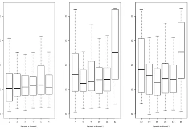
A boxplot of theStdError is shown in Figure 2. The mean of StdError is 16.2003, and the median is 16.6943. To put these values in perspective, let’s first consider the empirical distribution of priors in Period 1 of Round 1: (0,0,7,27,40,13,0,7,7,0). With such an empirical distribution a subject who assigns 100% to one of the extreme categories (C1 or
C10) and zero to all other categories would have a StdError of 35.5598, while a subject
who uniformly assigns 10% to each category would have a StdError of 12.7475. Hence subjects’ estimates are not too far off, but also have considerable errors. This suggests
that subjects perceive the scenario as ambiguous.
Second, we analyze the treatment effect between the ambiguous and the risky scenario.
Confidence distributions capture subjects’ perception of uncertainty with regard to other
subjects’ priors. In the ambiguous scenario, this uncertainty should contain subjects’
perception of ambiguity, which is our central focus. It could, however, also include the
lack of confidence in other subjects’ capability to understand the QSR, or the lack of
information about others’ risk attitudes, etc.. With the ambiguous scenario in isolation
we cannot distinguish between these confounding effects and the effect of ambiguity that
stems from the selected urn. But, as the same confounding effects also exist in the risky
scenario, a comparison of the standard deviations of the confidence distributions between
the ambiguous and the risky treatment can identify ambiguity as a separate component
of uncertainty in the confidence distributions.12 Indeed, a one-sided Wilcoxon rank-sum
test shows that the standard deviations of the confidence distributions of the ambiguous
scenario are significantly larger than those of the risky scenario (p < 0.01). Hence, subjects perceive the ambiguous scenario as more uncertain.
12
1 2 3 4 5 6
10
15
20
25
30
Periods in Round 1
7 8 9 10 11 12
10
15
20
25
30
Periods in Round 2
13 14 15 16 17 18
10
15
20
25
30
[image:18.595.111.497.259.526.2]Periods in Round 3
3.2 Static analyses
3.2.1 Multiple priors and single priors
With the interpretation of subjects’ confidence distributions as a probability measure of
their multiple priors we can now analyze how a subject’s single prior relates to her multiple
priors. Although it is intuitive to assume that the aggregation of multiple priors into a
single prior is analogous to the way how multiple priors enter an asset valuation, there
is no theory for this. Multiple prior models attempt to directly explain valuations (see
Section 3.2.2 for tests), but they stay silent on how subjects would aggregate multiple
priors into a single prior. On a more exploratory note we therefore investigate, whether
subjects, when forced to state a single prior, report the min of their multiple priors, the
max of their priors, the prior in which they are most confident, or perhaps a confidence
weighted average of all multiple prior.13
To see which selection or aggregation of multiple priors best explains subjects’ reported
single priors, we compute the mean difference, mean standard error, as well as the
Spear-man correlation between each of the measures mentioned above and subjects’ single prior.
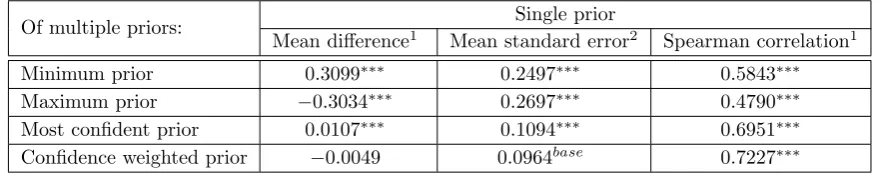
As the results in Table 3.2.1 show, the confidence weighted prior has the smallest mean
difference, mean standard error, and the highest correlation with the single prior. The
standard errors regarding the confidence weighted prior are significantly smaller than those
of the minimium prior, the maximum prior, and the prior that subjects are most
confi-dent in (one-sided paired Wilcoxon signed-rank tests,p <0.01 for all tests). Thus, when subjects are asked to state only one prior, they seem to report their confidence weighted
multiple prior.
This suggests a surprisingly high degree of sophistication in the aggregation of multiple
priors under ambiguity. As confidence weighted priors are closest to a Bayesian approach of
dealing with ambiguity, our result is very much in line with recent, mostly neuroscientific
studies that find support for the view that many processes in the brain are Bayesian
13
Of multiple priors: Single prior
Mean difference1 Mean standard error2 Spearman correlation1
Minimum prior 0.3099∗∗∗ 0.2497∗∗∗ 0.5843∗∗∗
Maximum prior −0.3034∗∗∗ 0.2697∗∗∗ 0.4790∗∗∗
Most confident prior 0.0107∗∗∗ 0.1094∗∗∗ 0.6951∗∗∗
Confidence weighted prior −0.0049 0.0964base
0.7227∗∗∗
∗∗∗,∗∗,∗, denote statistical significance at the 1%, 5%, and 10% level, respectively.
[image:20.595.85.524.86.173.2]1) Two-sided Wilcoxon sign-ranks test for equality of ’difference’ with zero (within each sample). 2) One-sided Wilcoxon sign-ranks test for a smaller standard error of the confidence weighted prior.
Table 1: Difference (single minus multiple), standard error, and Spearman correlation of the single prior with the min of multiple priors, the max of multiple priors, the prior that subjects are most confident in, and the confidence weighted prior.
(Friston, 2003, 2005; Doya et al., 2007).
3.2.2 Multiple priors and asset valuation
By analyzing the relationship between WTPs and multiple priors we can test multiple
models directly. Multiple prior models are an extension of the standard model, which
simply assumes expected utility and a single prior. We therefore specify, as a baseline
model, a random effects estimation with the reported single prior as the only explanatory
variable:
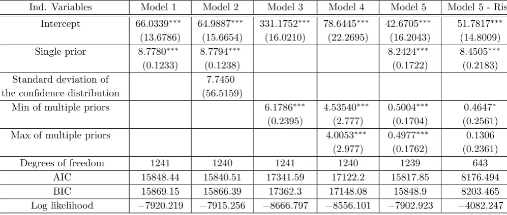
W T P s= Intercept +φi+β1m1+ǫ, (8)
wherem1 is the subject’s estimation that the true type of the selected urn is 1 and φi are
individual random effects on the intercept. Model 1 in Table 3.2.2 reports the results.
Note that a correct guess results in a payment of 1000 ECU and that the single prior is
reported in percent (m1 points out of 100). This means that a risk neutral subject would
be willing to pay 10 units more if her single prior increases by one percent. A reported
Ind. Variables Model 1 Model 2 Model 3 Model 4 Model 5 Model 5 - Risk
Intercept 66.0339∗∗∗ 64.9887∗∗∗ 331.1752∗∗∗ 78.6445∗∗∗ 42.6705∗∗∗ 51.7817∗∗∗
(13.6786) (15.6654) (16.0210) (22.2695) (16.2043) (14.8009)
Single prior 8.7780∗∗∗ 8.7794∗∗∗ 8.2424∗∗∗ 8.4505∗∗∗
(0.1233) (0.1238) (0.1722) (0.2183)
Standard deviation of 7.7450
the confidence distribution (56.5159)
Min of multiple priors 6.1786∗∗∗ 4.53540∗∗∗ 0.5004∗∗∗ 0.4647∗
(0.2395) (2.777) (0.1704) (0.2561)
Max of multiple priors 4.0053∗∗∗ 0.4977∗∗∗ 0.1306
(2.977) (0.1762) (0.2361)
Degrees of freedom 1241 1240 1241 1240 1239 643
AIC 15848.44 15840.51 17341.59 17122.2 15817.85 8176.494
BIC 15869.15 15866.39 17362.3 17148.08 15848.9 8203.465
Log likelihood −7920.219 −7915.256 −8666.797 −8556.101 −7902.923 −4082.247
∗∗∗,∗∗,∗, denote statistical significance at the 1%, 5%, and 10% level, respectively.
[image:21.595.94.593.86.298.2]Heteroskedasticity-consistent standard errors are reported in parentheses.
Table 2: Random effects regression of WTPs and priors, min (and/or max) of multiple priors.
that many subjects report a value of 0.5 as single prior. Yet, among these subjects, there is a high degree of heterogeneity in their multiple priors and WTPs. Figure 3 shows
that these values can be vastly different, despite the fact that all the subjects considered
reported a prior of 0.5. In Models 2 to 4 we therefore analyze the potential impact of multiple priors and their confidence distributions.
In Model 2 of Table 3.2.2 we first investigate whether the perceived level of uncertainty has
an effect on the evaluation of ambiguous assets. In particular, a high level of uncertainty
could have a negative (positive) effect on the evaluation by ambiguity averse (seeking)
subjects (Klibanoff et al., 2005; Nau, 2006). To examine this, we include the standard
deviation of the confidence distribution on multiple priors in the empirical specification.
In the spirit of Klibanoff et al.’s (2005) model and Nau’s (2006) model, and with a majority
of subjects being ambiguity averse, we would expect a negative coefficient of the standard
deviation. However, as the results of Model 2 show, the coefficient is not significant
(p >0.10) and has the opposite sign.
Model 3 replicates the maxmin model by including the minimum of the multiple priors as
The min of multiple priors conditional on a prior of p=0.5
The min of multiple priors
Frequency
10 20 30 40
0
20
40
60
The max of multiple priors conditional on a prior of p=0.5
The max of multiple priors
Frequency
40 50 60 70 80 90
0
20
40
60
WTPs conditional on p=0.5
WTPs
Frequency
300 400 500 600 700 800
0
10
20
30
40
[image:22.595.99.487.256.517.2]50
significant, the explanatory power of the model decreases dramatically, in terms of AIC,
BIC, and Log likelihood criteria. As suggested by theα maxmin model, the specification in Model 4 additionally includes the max of multiple priors. In line with the α maxmin model, the max of priors (4.0053) plays a statistically and economically important role. However, the overall explanatory power of the Model 4 is relatively weak.
Thus, we do not find exclusive support for either of the two multiple priors models (Model
3 and 4), nor for Nau’s (2006) model, but strong economic significance and explanatory
power when including single priors (Model 1 and 2). In Model 5, we therefore examine
the maxmin model andα maxmin model in combination with single priors. The maxmin model argues that subjects only use the min of multiple priors for their evaluation, even if a
single prior and the max of multiple priors are available. However, according to the results
for Model 5, both coefficients for the min and the max of multiple priors are statistically
significant (with p ≤ 0.01) and economically important (0.5004 for the min, 0.4977 for the max of priors)., though the coefficient for the max of priors is slightly smaller. Thus,
both the min and the max of multiple priors, as well as the single prior, contain useful
information in explaining the values of the ambiguous assets. In fact, Model 5 has the
highest explanatory power in terms of AIC, BIC and Log likelihood.14 When we estimate
the same model with the sample of refined subjects, the coefficient for the min of priors
stays significant while the coefficient for the max of priors loses its significance (0.7368 for the min of the priors with p < 0.01, 0.2909 for the max of the priors with p >0.1). Note that the single prior still plays an important role. With a value of 8.2424, its effect is only slightly lower than in Model 1 (8.7780) and clearly higher than the min (0.5004) and the max (0.4977) of priors. This is not consistent with the suggestion of the maxmin model (α maxmin model) that only the min of multiple priors (the min and the max) has explanatory power for the value of ambiguous assets. When comparing the maxmin
model and theα maxmin model, the results provide more support for the latter, because subjects consider both the max and the min of multiple priors. In doing so, they seem to
place some more weight on the min of priors.
As discussed in Section 3.1, the dispersion of the confidence distributions may contain
14
multiple components of uncertainty, including subjects’ own perception of uncertainty in
the ambiguous scenario, and uncertainties regarding others, e.g., subjects’ risk attitudes
and their capability to understand the QSR. However, note that, in principal,
uncertain-ties regarding others should not play a role when one obtains an own valuation of the ambiguous asset. If the dispersion of the confidence distributions only reflects uncertainty
about the second component, it should not have any explanatory power for the WTPs.
This claim is based on the assumption that there is no common factor which influences
both the way subjects report uncertainties regarding others and their own evaluation.
To test this claim, we run a random effects regression similar to Model 3, but with the
data of the risky treatment. As the results in Model 5-Risk show, the coefficient for the
min of priors is only weakly significant (p = 0.0701), and the effect size is smaller than in the ambiguous treatment (0.5004 vs 0.4647), in particular when we consider only the refined subjects (0.7368 vs 0.4647). This suggests that the min of priors in the ambiguous treatment genuinely captures some additional information.
3.3 Updating
3.3.1 Updating of single priors
We first examine the updating of single priors. As a starting point, we check whether
subjects adjusted the reported probability in accordance with the signals (the color of the
drawn balls). This provides a first indication whether the quadratic scoring rule was well
understood by the subjects. Figure 4 reports subjects’ single priors that the randomly
selected urn was of Type 1 (3 black balls and 6 white balls).15
Figure 4 suggests that the priors respond to the drawn ball sequence in the right direction.
For example, in Round 1 the ball sequence was BBWWB. Subjects start with a median
prior of 0.5 before seeing any balls, then lower the stated prior after seeing black balls
in Period 2 and 3, then raise their prior after seeing white balls in Period 4 and 5, and
15
1 2 3 4 5 6
0.0
0.2
0.4
0.6
0.8
1.0
Periods in Round 1
First−order subjectiv
e beliefs
Ball sequence: B,B,W,W,B
7 8 9 10 11 12
0.0
0.2
0.4
0.6
0.8
1.0
Periods in Round 2
First−order subjectiv
e beliefs
Ball sequence: B,W,B,B,B
13 14 15 16 17 18
0.0
0.2
0.4
0.6
0.8
1.0
Periods in Round 3
First−order subjectiv
e beliefs
[image:25.595.102.496.251.514.2]Ball sequence: W,W,W,B,W
finally decrease the prior again after a last black ball in Period 6. Similar developments
can be observed in Round 2 and 3. Thus, subjects recognized the information content
of the signals and reacted accordingly. A paired two-sided Wilcoxon signed-ranks test of
the empirical priors and one-period Bayesian updated priors suggests that the updating
process is not significantly different from a Bayesian process (p > 0.10).16 This result is consistent with Bossaerts et al. (2010), who assume Bayesian updating for a (uniform)
prior in an ambiguous scenario and find that such an assumption fits their data well.
As mentioned in the introduction, pertinent literature suggests that individuals update
differently when receiving a confirming signal (a signal that is identical to the previous
signal) than receiving a contradictory signal (a signal that opposes the previous signal).
To test this hypothesis, we calculate the updating errors: that is, the observed updating
minus one-period Bayesian updating after a confirming signal (in Period 3, 5, 11, 12, 15,
16), and after a contradictory signal (in Period 4, 6, 9, 10, 17, 18). We then compare
the updating errors after a confirming signal with those after a contradictory signal. The
mean updating error after a confirming signal is −2.3694 percent, and 1.9603 percent after a contradictory signal. A two-sided Wilcoxon rank-sum test suggests that the the
two samples of updating errors are significantly different from each other (p <0.01). Since negative errors imply ‘under-updating’ and positive errors ‘over-updating’, subjects seem
to overadjust their beliefs when receiving a contradictory signal and underadjust to a
confirming signal in the ambiguous scenario. This result seems to be consistent with the
claim that investors react more strongly to bad news than to good news (Epstein and
Schneider, 2008; Illeditsch, 2011).17
16
In one-period Bayesian updating, posteriors are Bayesian updated from the one-period ahead priors. An alternative would be to use the first period beliefs as the priors to calculate Bayesian posteriors for all later periods. For instance, the Period 6 Bayesian posteriors would be updated all the way from the first period beliefs, instead of being updated from the beliefs one period ahead – Period 5 – as in one-period Bayesian updating.
17
Note that a confirming signal can be bad news if it confirms a lower value of the selected urn. Therefore, our notation of confirming and contradictory signals cannot be directly translated into good or bad news. Learning, however, may provide a link, because subjects’ confidence about the underlying state of the world increases with a confirming signal while it decreases with a contradictory signal. This tendency is weaker in the risky treatment, where the mean updating error after a confirming signal is−1.8509 percent
(−2.3694 under ambiguity) and the mean updating error after a contradictory signal is 0.5395 percent
(1.9603 under ambiguity). Moreover, and in contrast to the ambiguous scenario, the difference between
3.3.2 Updating of multiple priors
As shown in Section 3.1, a typical feature of the ambiguous scenario is the larger standard
deviation of the confidence distributions of multiple priors. A larger standard deviation
signals less confidence in any of the multiple priors. This lack of confidence could affect
the way subjects update their priors. To test this, we first calculate the absolute difference
between observed updated priors and one-period Bayesian updated priors. A Spearman
correlation test between subjects’ absolute updating errors and the standard deviations
of their confidence distributions shows a significant positive correlation of ρ = 0.1213 (p <0.01). This suggests that subjects who are less confident in their priors make larger updating errors.
A signal not only changes subjects’ priors, it should also change their confidence
distri-bution of multiple priors. When a white (black) ball is drawn, it becomes more (less)
likely that the selected urn is of Type 1 and the confidence distributions of multiple priors
should be updated upwards (downwards), in the sense of first-order stochastic dominance.
Let P rior(¯pi|W) (P rior(¯pi|B)) denote the prior that would obtain the Bayesian
poste-rior of ¯pi after a white (black) ball.18 Using equations (7) and (6), and the fact that
the proportion of black balls in S1 is q1 = 13 and in S2 is q2 = 23, it can be shown that
P rior(¯pi|W) = p¯i
·(1−q2)
(1−q1)−¯¯p(qi 2−q1)
= 2−p¯ip¯i and P rior(¯p
i|B) = p¯i
·q2
¯ pi
i(q2−q1)+q1 =
2¯pi
1+¯pi. Since
¯
¯p1= 0.10,p¯2 = 0.20, . . . ,p¯9 = 0.90, we obtain the following values.
• When a white ball is drawn:
P rior(¯pi|W) = 0.05,0.11,0.18,0.25,0.33,0.43,0.54,0.67,0.82.
That means priors in the range of [0.05,0.11) should be updated (upwards) to the range of [0.10,0.20), and priors in the range of [0.11,0.18) should be updated to the range [0.20,0.30), and so on.
• When a black ball is drawn:
18
P rior(¯pi|B) = 0.18,0.33,0.46,0.57,0.67,0.75,0.82,0.89,0.95.
That means priors in the range of [0.01,0.18) should be updated (downwards) to the range [0.01,0.10), and priors in the range of [0.18,0.33) should be updated to the range [0.10,0.20), and so on.
Figure 5 displays the updating errors in each belief interval, computed as observed
updat-ing minus Bayesian updatupdat-ing. We consider only periods with belief updatupdat-ing, e.g., Period
2, 3, 4, 5, 6 in Round 1, Period 8, 9, 10, 11, 12 in Round 2, and Period 14, 15, 16, 17,
18 in Round 3. As Figure 5 shows, in most intervals the median updating error is zero,
which indidicates that updating in the confidence intervals is approximately Bayesian.19
2 4 6 9 12 16
−40
−20
0
20
40
2 4 6 9 12 16
−40
−20
0
20
40
2 4 6 9 12 16
−40
−20
0
20
40
2 4 6 9 12 16
−40
−20
0
20
40
2 4 6 9 12 16
−40
−20
0
20
40
2 4 6 9 12 16
−40
−20
0
20
40
2 4 6 9 12 16
−40
−20
0
20
40
2 4 6 9 12 16
−40
−20
0
20
40
2 4 6 9 12 16
−40
−20
0
20
40
2 4 6 9 12 16
−40
−20
0
20
[image:28.595.107.499.334.592.2]40
Figure 5: Updating error in each category: Empirical updating - Bayesian updating. Only periods where belief updating takes place are considered. That is, periods 2,3,4,5,6 in Round 1, periods 8, 9, 10, 11, 12 in Round 2, and periods 14, 15, 16, 17, 18 in Round 3.
19
We now consider the standard deviations of subjects’ confidence distributions, which can
be interpreted as subjects’ perception of uncertainty in an ambiguous scenario. Epstein
and Schneider (2007) suggest that individuals’ confidence about the ambiguous
environ-ment changes as they learn. Such a change in confidence may depend on the signals
received, in particular, whether they are confirming or contradictory. To analyze this,
we computethe updating errors of subjects’ empirical confidence distributions, that is the
standard deviations of the empirical confidence distributions minus the standard
devi-ations of the one-period Bayesian updated confidence distributions. We find that the
mean updating error after a confirming signal is 0.0037, and−0.0133 after a contradictory signal. Both updating errors are statistically significant from zero (two-sided Wilcoxon
signed-ranks test, p = 0.0143 for confirming signals and p < 0.01 for contradictory sig-nals). Thus, when receiving a confirming signal, subjects’ areless confident (and perceive more uncertainty) than implied by Bayesian updating, because the standard deviation
of subjects’ observed confidence is still greater than implied by Bayesian updating (with
a mean difference, or updating error, of 0.0037). When receiving a contradictory signal, however, subjects’ aremore confident (and perceive less uncertainty) than they should un-der Bayesian updating (with a mean difference in standard deviations of−0.0133). This feature of updating in the confidence distributions is similar to the updating of single
pri-ors as described in Section 3.3.1. Subjects seem to underadjust (overadjust), both, their
confidence and their single priors, when receiving a confirming (contradictory) signal.
Finally, we examine the updating of the confidence distributions after receiving the same
information overal, but with different signal sequences. Note that our ambiguous scenario
is essentially the Scenario 2 in Epstein and Schneider (2007): the true state of the world
– though ambiguous – is fixed, and thus should be revealed through learning in the long
run. More specifically, subjects initially have little information about the true state of the
world. Due to the lack of information, subjects have weak confidence in their priors. This
is reflected in large standard deviations of subject’s confidence distributions. After balls
are drawn, the true state of the world is slowly revealed. For example, subjects may believe
to know more after seeing the signal sequence of “BBWW” than without seeing anything.
This knowledge cannot be exhibited in priors because subjects’ priors should be the same
Pairs of signals Ambiguous treatment Risky treatments
Mean Comparison p−value Mean Comparison p−value
0 vs BBWW in Round 1 0.1628 v 0.1374∗∗∗ 0.0035 0.1273 v 0.1050 0.2087
B vs BBW in Round 1 0.1486 v 0.1415∗ 0.0578 0.1192 v 0.1091 0.1870
B vs BBWWB in Round 1 0.1486 v 0.1377∗∗ 0.0226 0.1192 v 0.1021 0.1124
BBW vs BBWWB in Round 1 0.1415 v 0.1377 0.2451 0.1091 v 0.1021 0.3302
0 vs BW in Round 2 0.1244 v 0.1213 0.1737 0.1008 v 0.0954 0.1904
B vs BWB in Round 2 0.1270 v 0.1206∗∗ 0.0177 0.1048 v 0.1053 0.3408
WWW vs WWWBW in Round 3 0.1156 v 0.0823∗∗∗ 0.0000 0.1056 v 0.0799∗∗ 0.0163
∗∗∗,∗∗,∗, denote statistical significance at the 1%, 5%, and 10% level, respectively.
[image:30.595.86.542.85.213.2]B=Black ball; W=White ball; 0=No signal
Table 3: One-sided paired Wilcoxon signed-ranks tests on the standard deviations of subjects’ confidence distributions in situations with equal overall information.
priors. We therefore run one-sided paired Wilcoxon signed-ranks tests on the standard
deviations of subjects’ confidence distributions in pairs of situations where the revealed
information is essentially the same. As explained in Section 3.3.1, we have seven such pairs
in the experiment.20.In the spirit of Epstein and Schneider (2007), subjects may have a
higher confidence level – reflected in lower standard deviations of confidence distributions
– in ambiguous situations with more signals, but no difference in overall information.
Table 3.3.2 reports the results. For all pairs the means of standard deviations of confidence
distributions are lower in the later period with more signals (second mean in each cell). In
the ambiguous treatment, the differences between the means are statistically significant
in 5 out of 7 comparisons. In the risky treatments, however, only one comparison is
statistically different. Hence the Null that more, but, in sum, neutralizing signals do not
matter, can be rejected for ambiguity, but seems to hold under risk.
4
Conclusion
This study is a first step towards understanding the evaluation of ambiguous assets and
belief updating in ambiguous scenarios where multiple priors are possible. We have
exper-20
imentally elicited each subject’s prior regarding the states of ambiguous scenarios. Since
there are only two states of world in our experimental framework, one probability
es-timation – the probability of the randomly selected urn being of Type 1 – completely
describes subjects’ probability measure of the states of the world, and hence is a prior of
the subject. To examine the possibility of multiple priors, in additional to each subject’s
prior, we elicited each subject’s other potential priors and the confidence distribution on
the multiple priors. We then discuss the relationship between subjects’ priors and their
multiple priors. We have also used subjects’ priors and their multiple priors to explain
subjects’ willingness to pay for the ambiguous assets, which are constructed on the same
underlying states as in the ambiguous scenarios. Finally, we have investigated how
sub-jects update their priors and their confidence distributions on multiple priors when they
received signals regarding the true state of the ambiguous scenarios.
We find that in ambiguous scenarios where multiple priors are possible, a subject’s prior,
when forced to state a single prior, is best understood as a confidence-weighted average
of multiple priors. In addition, we find that the valuation of ambiguous assets is best
ex-plained by subjects’ single priors, while the mins and the max’s of subjects’ multiple priors
also add explanatory power. This provides some, but no exclusive support for neither the
maxmin nor the α maxmin model. Further, belief updating after a confirming signal differs from that of a contradictory signal, both in terms of priors and confidence
distribu-tions of multiple priors. Subjects underreact (overreact) to confirmatory (contradictory)
signals, both in the updating of their prior, as in the adjustment of their confidence in
multiple priors. Finally, additional, but neutral information resolves uncertainty in the
sense of decreasing standard deviations of confidence distributions of multiple priors under
References
Bossaerts, P., Ghirardato, P., Guarnaschelli, S., and Zame, W. R. (2010). Ambiguity in
asset markets: Theory and experiment. Review of Financial Studies, 23(4):1325–1359.
Brier, G. (1950). Verification of forecasts expressed in terms of probability. Monthly Weather Review, 78:1–3.
Doya, K., Ishii, S., Pouget, A., and Rao, R. (2007). Bayesian Brain - Probabilistic Ap-proaches to Neural Coding. MIT Press, Cambridge, Massachusetts.
Ellsberg, D. (1961). Risk, ambiguity, and the savage axioms. The Quarterly Journal of Economics, 75(4):643–669.
Epstein, L. G., Noor, J., and Sandroni, A. (2010). Non-bayesian learning. The B.E. Journal of Theoretical Economics, 10(1):3.
Epstein, L. G. and Schneider, M. (2003). Recursive multiple-priors. Journal of Economic Theory, 113(1):1–31.
Epstein, L. G. and Schneider, M. (2007). Risk, ambiguity, and the savage axioms. Review of Economic Studies, 74:1275–1303.
Epstein, L. G. and Schneider, M. (2008). Ambiguity, information quality, and asset pricing.
Journal of Finance, 63(1):197–228.
Fischbacher, U. (2007). z-tree: Zurich toolbox for ready-made economic experiments.
Experimental Economics, 10(2):171–178.
Friston, K. (2003). Learning and inference in the brain.Neural Networks, 16(9):1325–1352.
Friston, K. (2005). A theory of cortical responses. Philosophical Transactions of the Royal Society B: Biological Sciences, 360(1456):815–836.
Ghirardato, P., Maccheroni, F., and Marinacci, M. (2004). Differentiating ambiguity and
ambiguity attitude. Journal of Economic Theory, 118(2):133–173.
Greiner, B. (2004). An Online Recruiting System for Economic Experiments. In: Kremer,
K., Macho, V. (eds.), Forschung und wissenschaftliches Rechnen 2003. GWDG Bericht
63, Goettingen, Gesellschaft f¨ur wissenschaftliche Datenverarbeitung: 79-93.
Guidolin, M. and Rinaldi, F. (2010). A simple model of trading and pricing risky assets
under ambiguity: any lessons for policy-makers? Applied Financial Economics, 20(1-2):105–135.
Hey, J., Lotito, G., and Maffioletti, A. (2010). The descriptive and predictive adequacy of
theories of decision making under uncertainty/ambiguity. Journal of Risk and Uncer-tainty, 41(2):81–111.
Illeditsch, P. K. (2011). Ambiguous information, portfolio inertia, and excess volatility.
Journal of Finance, 66(6):2213–2247.
Klibanoff, P., Marinacci, M., and Mukerji, S. (2005). A smooth model of decision making
under ambiguity. Econometrica, 73(6):1849–1892.
Marinacci, M. (2002). Learning from ambiguous urns. Statistical Papers, 43:145–151.
Nau, R. F. (2006). Uncertainty aversion with second-order utilities and probabilities.
Management Science, 52(1):136–145.
Offerman, T., Sonnemans, J., Kuilen, G. V. D., and Wakker, P. P. (2009). A truth
serum for non-bayesians: Correcting proper scoring rules for risk attitudes. Review of Economic Studies, 76(4):1461–1489.
Prelec, D. (2004). A bayesian truth serum for subjective data.Science, 306(5695):462–466.
Qiu, J. and Steiger, E.-M. (2011). Understanding the two components of risk attitudes:
An experimental analysis. Management Science, 57(1):193–199.
Routledge, B. and Zin, S. (2009). Model uncertainty and liquidity. Review of Economic Dynamics, 12(4):543–566.
Seo, K. (2009). Ambiguity and second-order belief. Econometrica, 77(5):1575–1605.
Trautmann, S. and Kuilen, G. v. d. (2011). Belief elicitation: A horse race among truth