A Measure of Early Warning of
Exchange-Rate Crises Based on the
Hurst Coefficient and the lpha-Stable
Parameter
Rodríguez-Aguilar, Román and Cruz-Aké, Salvador and
Venegas-Martínez, Francisco
Escuela Superior de Economía, Instituto Politécnico Nacional,
Escuela Superior de Economía, Instituto Politécnico Nacional,
Escuela Superior de Economía, Instituto Politécnico Nacional
2 October 2014
Online at
https://mpra.ub.uni-muenchen.de/59046/
A Measure of Early Warning of Exchange-Rate Crises Based
on the Hurst Coefficient and the
Αlpha
-Stable Parameter
Román Rodríguez-Aguilar
Escuela Superior de Economía, Instituto Politécnico Nacional
Salvador Cruz-Aké
Escuela Superior de Economía, Instituto Politécnico Nacional
Francisco Venegas-Martínez
Escuela Superior de Economía, Instituto Politécnico Nacional
Abstract
The Hurst coefficient and the alpha-stableparameter are useful indicators in the analysis
of time series to detect normality and absence of self-similarity. In particular, when
these two features met simultaneously, it is said that the series is driven by white noise.
This paper is aimed at developing an index to measure the degree to which a time series
departs from white noise. The proposed index is built by using the principal component
analysis of the Mahalanobis distances between the Hurst coefficient and the alpha-stable
parameter from theoretical values of normality and absence of self-similarity. A zero
value of the index corresponds to a pure white noise process, while a 100 value
correspond to the maximum distance between the actual series and the theoretical white
noise. The proposed index is applied to examine the exchange rate of the Mexican peso
against the USA dollar. When examining the exchange rate, one distinctive finding of
the Index is that it can be used as an early warning indicator of crises, as it is shown for
the Mexican case.
JEL Classification: G15, F31, C43 and C53.
Introduction
Reality can barely be described by any mathematical model because of the abstraction
procedure. Most models in economics and finance usually rely on two idealistic
assumptions, independence and normality. Regrettably, none of these two assumptions
are ever entirely fulfilled. In fact, the existence of heavy tails, volatility clusters, and
other persistence phenomena becomes the rule more than the exception.1 Maybe the
most outrageous fact in analysis of financial time series is that they do not seem to be
identically distributed along time. In fact, they do not seem to present any predictable
structure since they are influenced by many external uncertainty sources.
On the other hand, it is well known that the Hurst coefficient and the
alpha-stable parameter allow us to identify the self-similarity and the degree of impulsivity in
a time series. It is worth noticing that both phenomena are related but they are not the
same. In fact, we can see a single heavy tail realization associated to a single event or a
volatility cluster contained on a certain range. This seems to be the case when a crisis is
not declared but the market remains on the lookout. A worthy microeconomic
explanation of this relationship is given in Lux and Marchesi (2000), in which the
excess of kurtosis and volatility clusters arise as a response to the heterogeneity of
economic agents in simulated artificial markets. Also Kirchler and Huber (2007) found
that the asymmetry in information is a major source of excess kurtosis in their simulated
artificial market. Also, a financial explanation to this matter is given in Thurner et al.
(2012) elucidating that the fat tails phenomena is a response to the urgent margin calls
to close leveraged positions. As it can be perceived, even when both phenomena are
related, they describe different ways of departing from normality. This is why it is
desirable to have a single measurement that indicates how far the actual time series is
from the white noise assumption. Moreover, detecting how far a time series (in
particular the exchange rate series) is from being white it can be useful to detect patterns
of crisis preludes, which is an important issue in finance and economics. In this regard,
the econometric based methods as proposed by Oh et al. (2006) interpret some
predetermined volatility patterns as crisis preludes. Also, Al-Anaswah and Wilfling
1
Very well-known surveys on this non white noise characteristics can be found on Mandelbrot (1963),
(2011) propose a Markov switching model of the present value of the stock prices to
statically detect the bubble burst states. Meanwhile, Gürkaynak (2008) collects and
reviews the most used econometric techniques for bubble detecting, and Lim et al.
(2008) use a bicorrelation test in order to prove market efficiency during the Asian
crises on seven selected Asian markets. Finally, we mention the work of Harvey et al.
(2013) that use a unit root test approximation to detect the bubble burst. In most of these
studies, the proposed methodology relies on the existence of the second moment of the
distribution, which is not always feasible when there are fat tails. Even more, if the data
is not normal, there may be some important information on the higher order sample
moments that is not being considered only in the variance.
Other crisis detection models are based on non linear assumptions, as the jump
diffusion detection method proposed by Andersen and Sornette (2004), the entropy
based measure as suggested by García-Ruiz et al. (2014), and the oscillator
methodology as proposed by Chian (2000). In all these cases, the models are able to
capture some of the higher order dependence (depending on the model), but they are not
giving a direct measurement of how far is the time series from the white noise
assumption.
Our proposal can be classified as non-linear and non-normal approach. The use
of the principal component analysis responds to the necessity of “cleaning the
overlapping explanation” between both elements. As we state previously, the existence
of fat tails is not necessarily associated with the volatility clusters and vice versa. The
non-normal characteristic of our model depends on the estimation of the alpha
parameter.2 This feature remains even when the data is sub-sampled quarterly or yearly
because the extreme value existence makes that the variance of a single observation
dominates the variance of the sample, thereby preventing the fulfillment of the central
limit theorem. Here, we need to elucidate that the consolidation of the data into low
frequency series, by using averages or other aggregation method, decreases the effect of
the outliers.
2
On the other hand, the non linearity characteristic (associated to long memory
properties) in our model is provided by the Hurst (1951) coefficient. This measurement
is related to the work of Cannon et al. (1997), Cheung and Lai (1995), and Cajueiro and
Tabak (2004). In their papers, they found the long memory feature only for the short
run or in variance. As in our proposal, the long memory effect seems to fade as the data
became of low frequency. The study of this fractal measurement and the long memory
effects is widely spread in Economics and Finance; see, for instance, Kulik and Soulier
(2011) describing the limiting behavior of tail empirical processes associated with long
memory stochastic volatility models. IN this regard, Mensi et al. (2014) analyze the
dual long memory properties of four major foreign exchange rate markets associated to
the world oil exporter Saudi Arabia using the ARFIMA–FIGARCH model. Other
example is that of Parthasarathy (2013) examining the long memory or long range
dependence in the Indian stock market vis-à-vis market efficiency; these are examples
of the current research on long memory associated with the Hurst coefficient or a related
measurement.
The proposed index will take into account the Hurst coefficient (memory
component) and the alpha parameter (heavy tails component). In fact, both concepts
were related in Jia et al. (2012) showing multi-fractal effects in the Shangai Stock
Exchange Composite Index, with longer memory associated to volatility clusters. Also,
Barany et al. (2012) relate a truncated Lévy flight distribution with the Hurst
coefficient. Likewise, Shrivastava and Kapoor (2013) relate a FARIMA process to the
existence of long memory by using the Hurst coefficient.
As it can be seen, our proposal incorporates the two main forms of deviation of a
stochastic process from white noise through a non-arbitrary measure, the Mahanalobis
distance, which incorporates in a structured way the relationship between the orthogonal
components of impulsivity (alpha coefficient component) and persistence (Hurst
coefficient component) of the analyzed time series as a way of detecting unusual market
movements, in a certain period, indicating the formation of a market disruption that may
be a sign of the prelude to a crisis. When examining the dynamics of the exchange rate,
one distinctive characteristic of the proposed Index is that it can be used as an early
The fact of choosing the exchange rate as the crisis indicating variable is not
arbitrary, as a high frequency variable its realizations can be used to feed a data
consuming tool as our proposal.3 It is also a difficult variable to be manipulated in the
long run by the monetary authorities, even with the recent use of derivatives based
exchange rate defense scheme; see, for instance, Neely (2001), Meaning and Zhu (2011)
and Fatum et al. (2013). The long run independence of the exchange rate makes it the
escape valve for the most of the imbalances between the local and rest of the world
economies. In addition to those properties, the exchange rate has proved to be a crucial
variable in the crisis analysis since the first crisis generation.4 In fact, the exchange rate
is a suitable indicator of how desirable and trustable is the local economy to both
foreign5 and local investors6, which can be turned into a predictor variable to the
investment GDP component analysis. On the consumption side, the exchange rate can
be understood as competitiveness and consumer’s confidence indicator as people buy
local goods if they are as good as their foreign competitors. Also, the public will buy
capital or durable goods (local and foreign) if they foresee future economic stability.7
The paper is organized as follows: in sections 2 and 3, we provide the theoretical
basis of the use of Hurst coefficient and alpha stable distributions, respectively; through
section 4, we show the usefulness of both parameters, separately, for characterizing the
impulsivity and memory of a financial time series and the necessity of incorporating
both features in our early warning crisis index; in section 5, we develop our Global
Index of Dissimilarity by using the Mahanalobis distance of Hurst coefficient and the
parameter α from a theoretical white noise for different periodicity (monthly, quarterly
and annual). With this information at hand, we compare our index with the actual
realizations of the Mexican peso-USD exchange rate to identify and analyze the crisis
3
Later, we will see that the Hurst coefficient calculations relies in the use of a LS regression that needs at least 25 observation points in order to avoid the micro-numerosity problem. On the other hand, the alpha stable distribution adjustment is made by means of a maximum likelihood, which requires a similar amount of data.
4
For more details on the crisis generations see, for instance, Belke and Schnalb (2013) or Kaminsky (2013).
5
Here we are making a reference to both, the capital account (short and medium run investment on financial instruments) and the foreign direct investment account (long run investment on physical capital).
6
If local investors are not willing to invest in their own country, there is a lack of confidence that will create a GDP or financial crisis.
7
periods; finally, in section 6, we present conclusions and acknowledge limitations of
this research.
2. Fractional Brownian motion and the Hurst coefficient
Brownian motion or geometric Brownian motion is a typical assumption made in
modern finance in order to describe the behavior of financial returns or an increasing
trend in the long run. The standard Brownian motion is a stochastic process with
continuous paths starting at zero, and whose increments are independent and normally
distributed.8 Roughly speaking, this assumptions denies the existence of fat tails, It also
rejects the persistence of the series because the independence of its increments. Despite
of their shortcomings, the Brownian motion assumption is widely used due to its
simplicity and because its tractability to obtain closed-form solutions when pricing
assets.9 Unfortunately, the behavior of financial time series does not necessarily fulfill
the Brownian or geometric Brownian motion assumptions.10 In general, financial time
series are non stationary and they present: discontinuities (jumps), volatility clusters,
kurtosis excess (heavy tails), bias, and long term dependency due self-similarity
As an alternative to overcome the weaknesses in the modeling assumptions
involved in the geometric Brownian motion, Mandelbrot (1997) proposed a model
called multi-fractal. This is based on the fractional Brownian motion. It was first
considered by Kolmogorov (1940), and its use became popular after Mandelbrot’s
(1965) work. The fractional Brownian motion of index ,
is a stochastic process satisfying:
almost everywhere
iii) The covariance of the process for two times s, t R is:
(1)
8
See Revuz and Yor (1999), Glasserman (2004). Closely related to the Brownian assumption is the geometric Brownian that can be viewed in Oksendal (2002), and Lamberton and Lapeyre (2007).
9
The shortcomings of the normality assumption are widely known; see, for instance, Lo and MacKinlay (2002).
10
The index H is called Hurst parameter11, which is a measure to characterize fractal sets.
Note that the Brownian motion can be obtained from standard fractional Brownian
motion if H = 1/2.
The fractional Brownian motion has no periodic cyclical variance in all time
scales, and takes into account the statistical dependence in the long term. In addition to
the typical characteristics of fractional Brownian Motion (FBM) mentioned above, we
shall use two features of fractal sets that give to the FBM a greater variability of
behavior12:
a) The self-affinity or statistical self-similarity. By reducing the time scale to
represent trajectories of the process. The appearance of the series is similar to
the number in the original scale.
b) Non integer value of the dimension. In characterizing the process is related to
the size variations experienced between neighboring points so that the higher the
value the greater dimension variation.
Accordingly, if a time series has a high dependency property, it should be modeled by
means of a fractional Brownian motion that, unlike traditional Brownian motion,
incorporates the features of dependence of financial series, starting with practically the
same assumptions of the traditional Brownian motion.
In order to relate the FBM used in many economic and financial applications, with
its fractal properties, the literature proposes the rescaled range , which is used to
determine the Hurst coefficient, H, associated to a time series. Hurst (1951) developed a
methodology13 applicable to time series that are not necessarily Brownian motion, but
presents long memory:
11
Referring to the British scientist Harold Edwin Hurst (1880-1978),
12
See, for instance, Mandelbrot and van Ness (1965), Beran(1994) and Comte and Renault (1996).
13
/ H
R S n cn
(2)
where:
Notation used for the rescaled range statistic,
c: is a proportionality constant,
n: is the number of interval data.
H: is the Hurst coefficient,
is a statistic with zero mean. The rescaled range starts with the series in the original order, and subsequently a new series is generated by taking the log difference
returns of the original data.
A) The series is dividedinto intervals of equal returns data number, the number of
intervalswill be called,hereinafter,“partitions”. So thatthe number of partitions
for the number of data is equal to the size range of the number of returns. By
varyingthe number of partitionswe obtaineach timeseriesdivided intointervals
of equalnumber of data.
B) Ineach partitionfor each ofthe ranges:
a. Calculate the mean and standard deviation.
b. Determine the variation of each data with respect to the mean and differences.
c. It sets the range of the data by subtracting the lowest to higher.
d. The range is divided by the standard deviation, obtaining the standardized range.
e. Use the identity14:
(3)
If the above formula is applied to all the possible partitions, then a MCO regression
is carried out to compute the Hurst coefficient, H, which is given by the slope of the
regression line, while the intercept, is the proportionality constant.
1. If 0 < H < , the series presents anti-persistency and mean reversion
characteristics. That is, if the series has been up to a certain value that serves as
14
For further reference see the seminal Hurst, Black and Simaika (1965) paper. Moreover, some Hurst
the long-term average in the previous period is more likely to be down in the
next period and vice versa, and this is named a pink noise.
2. If , the data are independent and do not have memory. This is a random
walk and it is called white noise, which is consistent with the Brownian motion.
3. If , the series is persistent. This means that it reinforces the trend and
so it presents long-term cyclical behavior15, and this process is called black
noise.
4. If H = 1, the series is deterministic.
Thus, the Hurst coefficient, H, is a parameter obtained by means of a MCO regression,
and as any other parameter, it is a conditional mean with the usual asymptotic and
normality characteristics. As stated in Greene (2003), the distribution of the estimated
vector of parameters, b, conditioned on the regressor matrix, X, with a sample size, n.
can be obtained form
' 1 1' ,
X X
n b X
n n
where is the vector of population parameters, and is the error vector. It can be
seen that given uncorrelatedness and independence on errors, , meeting the Grenader
conditions and using the central limit theorem,16 the MCO parameters, b, are normally
distributed as
1 2
'
, .
a X X
b N
n n
(4)
This means that if the previous conditions are met, the obtained Hurst coefficient is a
normal variable that can be tested using the Annis and Lloyd (1976) test for the Hurst
coefficient of a white noise stochastic process. The test is described by:
H0: The process is random and independent (H = 0.5).
H1: The process correlates (H≠ 0.5), and the test statistic given by
15
The color of the noise is given as a characteristic of its power spectrum, for more details see Kosko (2006).
16
(5)
It is important to point out that the Annis and Lloyd test (1976) is valid only under the
assumption of white noise, which fulfills the requirements for the normality of the
parameter vector of the MCO regression. There is a problem when the Hurst coefficient
is relatively near from the normality case, H= 0.5. In this case, there is a biasing
problem that can be large enough to invalidate a hypothesis testing but not so large to
reject the mean test specification because the test statistic is not in the tail of the
supposed distribution. This gives as a result a poor performance of the Annis and Lloyd
test for any other Hurst coefficient value distinct form H=0.5. This problem is analyzed
in Koutsoyiannis (2003) or Cajueiro and Tabak (2005)
2. Alpha-Stable Distributions
It is well known that financial time series present extreme value observations, which
characterizes the instability of a time series and denotes the presence of heavy tails
(impulsivity), which does not fulfill the requirements of the Central Limit Theorem. In
fact, they present a greater degree of impulsivity than that of the normal distribution;
extreme events, in Mexico, such as those in 1990, 2000, 2007 stock crashes are highly
unlikely to be driven from the normal distribution.
A very useful way of characterizing this impulsivity is the stable distributions
theory. It was first developed by Paul Lévy and Aleksander Khinchine, but, it was not
until the work of Mandelbrot (1963) and (1968) that the α-stable distributions were
popularized. Mandelbrot proposed a theory based on these distributions to explain the
acute price fluctuations observed in financial time series. In fact, by using standard
notation, it can be demonstrated that the normal17 , Lévy,
Landau, Holtsmark, and Cauchy,
distributions are special cases of the α-stable distributions. These
17
distributions, in general, cannot be written analytically18 but, due the recent
computational advances they had been recently rediscovered by many fields of the
science, for an insight on they applications see Feldman and Taqqu (1998) or Machado
Kiryakova and Mainardi (2011). A random variable, X, is a α-stable distribution iff it
shows the following characteristic function (Nolan, 2005):
exp 1 sign tan , 1
2
2
exp 1 sign log , 1
x i x i x
x
x i x w i x
(6)
where
and . In this characteristic function, α controls the degree
of impulsivity of the random variable X, while manages the symmetry of
distribution19, γ > 0 is a scale parameter (dispersion), and is the position parameter.
In this research, we will use the Nolan (2005) algorithm to estimate the alpha
stable distribution parameters. Nolan (1997) software is based on the Zotolarev (1986)
representation of the characteristic function. The idea of his software is to perform the
numerical integration of a set of splits of the random variable domain. These splits are
based on the sign change of the trigonometric functions (sinus and cosines) that result of
the transformation of Zotolarev’s (1986) representation20
into the complex plane.
It is important to point out that there are other methodologies for estimating the
parameters of an alpha-stable distribution, like those presented in Belov (2005)
proposing a combination of Gaussian and Laguerre quadratures; or Mittnik et al. (1999)
presenting an algorithm that applies the fast Fourier transform. Finally, DuMouchel
(1973) using a Bergström series expansion on the Zotolarev’s characteristic function
representation for approximating an alpha stable cumulative distribution.
18
The integral with respect to w of the alpha-stable characteristic function (6) only have an analytical solution for the described cases (Nolan, 2005).
19
A value 0represents a symmetrical α-stable distribution, while the values 1 and 1 represent positive and negative skewed α-stable distribution, respectively.
20The Zotolarev’s representation is based on a succession of Meijer G
After obtaining the α-stable distribution parameters, we will use the Anderson-Darling test in order to verify the fitting parameters. This test is used due to its
efficiency in the case of heavy tailed series; see, for instance, Kabasinskas and
Sakalauskas (2006) or Barbulescu and Bautu (2012).
3. The Hurst coefficient and the parameter
α
applied to the
Mexican peso-US Dollar exchange rate
By analyzing the Mexican peso-US Dollar exchange rate series in five cross sections
characterized by financial crises, the Hurst coefficient will be estimated and tested
whether there is independence of the time series or else if there is persistence or
antipersistence. The results are compared with the estimate of the parameter α of an
alpha-stable distribution, which identifies the impulsivity in the series. We expect that
in cases far from white noise, we will find fractal characteristics; this means some
degree of impulsivity, which is higher when there are extreme values and volatility
clusters.
Hurst coefficient and alpha parameter are estimated for the Mexican peso/US
Dollar exchange rate for different intervals of time. Time windows are constructed
based on the distinction of high volatility periods characterized by financial crises. The
methodology to calculate the Hurst coefficient is the rescaled range, applied to the
logarithmic returns of the Fix exchange rate Mexican peso-USD dollar during the
period 1992-2012. In this case, 180 partitions were conducted on average for each
period taking into account the number of observations in each cut; this is the maximum
number of partitions with the least possible loss of data, see Table 1.
For the adjustment of the alpha-stable distribution, it is considered a
parameterization, usually used for modeling financial data.21 By setting data into five
considered periods, we obtain the parameters characterizing the distribution by the three
generally methods used, i.e., quantiles, maximum likelihood, and regression, as in
Nolan (2005).
21
The estimated parameters by the regression method are presented with a
goodness of fit criterion to the data in accordance with the Anderson-Darling test. Note
that in all three methods used for five periods it is not rejected the hypothesis test H0:
the series follows the α-stable distribution. However, the regression method is mostly
[image:14.595.80.504.215.425.2]used in the analysis of financial series providing a best fit of the tails of the distribution.
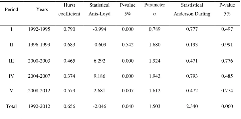
Table 1. Hurst coefficient and parameter α/1
Period Years Hurst coefficient
Statistical Anis-Loyd
P-value 5%
Parameter
α
Stastistical Anderson Darling
P-value 5%
I 1992-1995 0.790 -3.994 0.000 0.789 0.777 0.497
II 1996-1999 0.683 -0.609 0.542 1.680 0.193 0.991
III 2000-2003 0.465 6.292 0.000 1.924 0.471 0.776
IV 2004-2007 0.374 9.186 0.000 1.943 0.793 0.485
V 2008-2012 0.579 2.681 0.007 1.612 0.472 0.774
Total 1992-2012 0.656 -2.046 0.040 1.503 2.340 0.060
1 / To both the power of the statistical test used is affected by the number of data. The order of potency of the test is 34% to 250 data, 63% for 500 data and 83% for at least 1000 observations. Data from Banxico
In what follows, parameters are compared statistically. For the case of Hurst coefficient
it is used the Anis-Loyd statistic, and for the case of α-stable it is used the distribution
Anderson-Darling test; both at 95% confidence. The obtained results show that the
Hurst coefficient was statistically different from 0.5, with the exception of period II,
which shows that the series is not independent over time. In the case of the α-stable
distribution, in all periods, we cannot reject the hypothesis that the series is α-stable
distributed. It is important to detect if the series presents impulsivity and time
dependence. The existence of those two characteristics may lead to errors in the
estimates; this is the main reason because we cannot use normality and independence
assumptions indiscriminately. Both indicators are related in their implications towards
determining a range analysis. In the case of presence a fractal behavior, it is convenient
to use the fractional Brownian motion. The characterization of a series based on these
two parameters will determine the correct methodological analysis and will help to
assumptions, namely, independence and normality.
4. The use of the Hurst coefficient and the parameter
α
as
early warning indicators
In this section, the Hurst coefficient and the parameter α will be calculated monthly,
quarterly and annually for the daily exchange rate during the period 1992-2012. First,
we present the Hurst coefficient for different time intervals. Next, we estimate the α
parameter for the time series in question and, finally, we discuss the dissimilarities
between the estimates. We compare the parameter determining a random walk in the
Hurst coefficient and contrast the normal case with the parameter α. With both
indicators providing dissimilarities of their theoretical parameters, we will construct an
index of early warning crises by using multidimensional scaling.
4.1 The Hurst coefficient estimation
The Hurst coefficient is estimated for the series of Fix exchange rate Mexican peso-US
Dollar during 1992-2012 with daily data. In particular, we analyze the data
independence with the rescaled range methodology using the maximum number of
possible partitions with less data loss. The Hurst coefficient shows a persistence and
antipersistence in episodes of high volatility. We can observe that the coefficient
estimation using monthly partitions is close to 1, denoting a kind of determinism in the
time series, however, there is some evidence that states that using the technique of
rescaled range in small series, the parameter estimates may be overstated (Hastings and
Sugira, 1993).
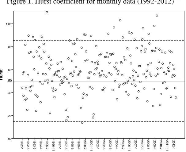
The observed values for monthly data indicates the presence of few values where
the Hurst coefficient is consistent with the random walk, H = 0.5, denoted by the solid
line. In fact, a lot of them show long memory (70% of data are above the solid line)
Figure 1. Hurst coefficient for monthly data (1992-2012)
Source: Author’s own elaboration with Banxico data.
For the case of quarterly estimates, the Hurst coefficient values rarely are observed near
of the top limit (1). In fact, they are clustered around the white noise solid line, (H =
0.5) but there remains some long memory observations and some observations below
the solid line (70% of data shows persistence and 30% antipersistence, it remains the
Figure 2. Hurst coefficient for quarterly data (1992-2012)
Source: Author’s own elaboration with Banxico data.
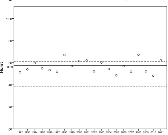
For annual data, Hurst coefficient reflects the varying results in the same sense as in the
two previous periodicities but with higher clustering effect. It is clear that the more data
is used to estimate the coefficient, the higher will be the robustness of the parameter.
Figure 3. Hurst coefficient for annual data (1992-2011)
[image:17.595.160.444.475.703.2]Only in two years, 1999 and 2006, the Hurst coefficient has values close to the white
noise. In other periods show persistence and anti-persistence; especially in those years
identified as periods of crisis.
4.2 Estimation of the parameter
α
The parameter α was estimated based on the software developed by J. P. Nolan
estable.exe. The adjusted α-stable distribution parameters were fitted to the exchange
rate Mexican peso-US Dollar. Particularly the parameter α, will tell if a series is
impulsive. It also indicates the presence of outliers or heavy tails; this phenomenon is
associated in financial series with high volatility or stress periods. We emphasize that
we used the parameterization.22 Adjustment parameters of the data were obtained by
characterizing the distribution with the three more commonly used methods, namely:
quantile, maximum likelihood, and regression (Nolan, 2005). In this case, the regression
method is preferred due to its better adjustment of the tails of the distribution.
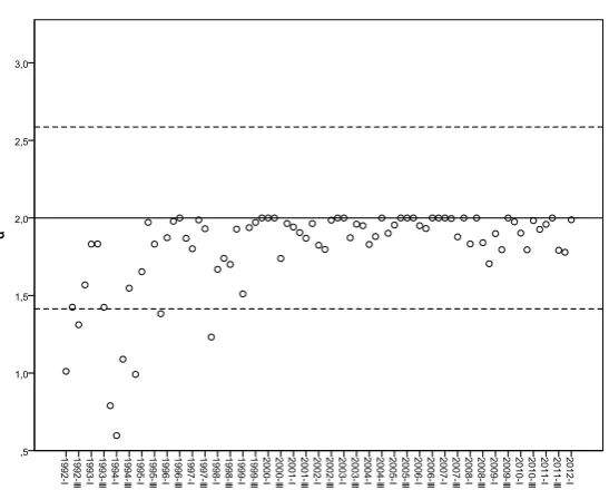
As it can be seen in Figure 4, there are several observations near to the normal
case, which are showed with the solid line on α = 2. In this case, the series does not
present a high degree of impulsiveness and, therefore, there are not heavy tails on the
distribution. It is noteworthy that there are periods where the parameter α is close to the
normal case. This allows the differentiation of cases depending on the behavior of the
parameter α for the construction of an early warning index. This can be clearly seen in
the observations where the alpha parameter is visibly far from 2. Finally, is important to
mention that in all cases, there is a stress period in the exchange market as in 1994.
22
Figure 4. Parameter α for monthly data (1992-2012)
Source: Author’s own elaboration with Banxico data.
In consistency with the estimated Hurst coefficient, the less volatile periods have values
close to H = 0.5 and α = 2. The cases consistent with the white noise assumption that
are less impulsive are associated with these observations. As in the case of the Hurst
coefficient, the estimated α parameter on a quarterly basis shows less impulsivity that
that of monthly observations.
Figure 5. Parameter α for quarterly data (1992-2012)
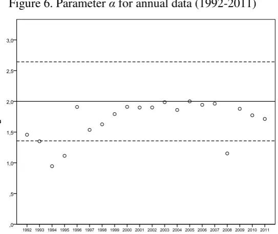
[image:19.595.166.440.517.737.2]Using annual frequency data, it can be seen a trend towards normality that was
significantly broken by the 1994-1995 and 2008 crises when de α parameter drops to 1.0
and 1.1 respectively. After that, the annual parameters remain in a range between 1.4
[image:20.595.168.440.199.428.2]and 2.
Figure 6. Parameter α for annual data (1992-2011)
Source: Author’s own elaboration with Banxico data.
Finally, we want to emphasize that the impulsivity periods are exactly the same that
presents long memory behavior. The estimation of these two parameters allows the
verification of the white noise assumption and the determination of error sources.
5. Early Warning Indicators
By considering that data with low impulsivity and no dependence over time, satisfy,
respectively, H = 0.5 and α = 2, it is possible to quantify the contrast between these
parameters by choosing the Mahalanobis distance as a measure of this dissimilarity.
The Mahalanobis ranges from 0 to 1, and it is calculated as the distance between the
individual observations and a parameter vector. Mahalanobis dissimilarity was chosen
since it meets the following essential properties (Cartera, 1998): non negativity,
symmetry, and triangle inequality. It is invariant under nonsingular linear
variables, for two variables is greater than for a single, decreasing with increasing
correlation between variables.23
In order to have a magnitude of how far is the data in each period of the normal
case and the level of independence of the data (or self-similarity), we construct a graph
of dissimilarities for both parameters using the Mahalanobis dissimilarity measure
[image:21.595.97.515.240.400.2]estimated from the normal case to the actual data.
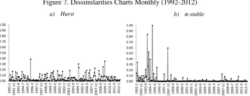
Figure 7. Dissimilarities Charts Monthly (1992-2012)
a) Hurst b) α-stable
Source: Author’s own elaboration with Banxico data.
As shown in Figure 7, the dissimilarity between the parameters increases in those cases
where there are periods of high volatility, which were crisis years. The parameter α is
far from to 2 determining impulsivity in the series. We can see this phenomenon in the
crisis of 1995, and in every monthly observation associated to market stress moments.
In all cases, the impulsivity measurement of the alpha parameter corresponds to a high
Hurst coefficient.
The graph of dissimilarities allows us to know, in an analytical way, when the
normality assumption is not met, and, as a consequence, the normal based estimations
or forecasts are neither accurate nor reliable. This happens especially during market
stress periods. When analyzing the quarterly estimated dissimilarities, we see that the
behavior of Mahalanobis distance is consistent with the monthly estimated
dissimilarities. The estimated parameters deviate from the theoretical values in periods
23
For further details see Mahalanobis (1936), Cartera, (1998), and McLachlan (2004).
of crisis and high volatility of the exchange rate. Again, the departures from the
normality assumption can be easily viewed in both the Hurst coefficient and the alpha
[image:22.595.88.523.159.349.2]parameter.
Figure 8. Dissimilarities Charts Quarterly (1992-2012)
a) Hurst b) α-stable
Source: Author’s own elaboration with Banxico data.
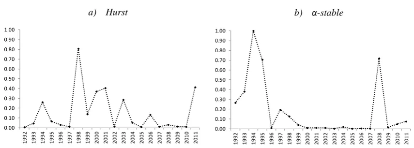
For the annual event dissimilarities, the graph shows a similar trend than in the previous
data frequencies. The differences between the estimated parameter and the parameters
consistent with the normal and independence assumptions are larger in the years when
there is high volatility in the series.
Figure 9. Dissimilarities Charts Annual (1992-2011)
a) Hurst b) α-stable
Source: Author’s own elaboration with Banxico data.
A key discussion element is that the dissimilarities charts provide a scale in which we
can see how far the actual parameters are from their theoretical vales. This allows us to
0.00 0.10 0.20 0.30 0.40 0.50 0.60 0.70 0.80 0.90 1.00 1992 -I 1993 -I 1994 -I 1995 -I 1996 -I 1997 -I 1998 -I 1999 -I 2000 -I 2001 -I 2002 -I 2003 -I 2004 -I 2005 -I 2006 -I 2007 -I 2008 -I 2009 -I 2010 -I 2011 -I 2012 -I 0.00 0.10 0.20 0.30 0.40 0.50 0.60 0.70 0.80 0.90 1.00 1992 -I 1993 -I 1994 -I 1995 -I 1996 -I 1997 -I 1998 -I 1999 -I 2000 -I 2001 -I 2002 -I 2003 -I 2004 -I 2005 -I 2006 -I 2007 -I 2008 -I 2009 -I 2010 -I 2011 -I 2012 -I 0.00 0.10 0.20 0.30 0.40 0.50 0.60 0.70 0.80 0.90 1.00
1992 1993 1994 1995 1996 1997 1998 1999 2000 2001 2002 2003 2004 2005 2006 2007 2008 2009 2010 2011 0.00 0.10 0.20 0.30 0.40 0.50 0.60 0.70 0.80 0.90 1.00
[image:22.595.86.514.511.664.2]set thresholds for financial analysis. Note that in the case of the estimation of both
parameters at all frequencies we are not contrasting their statistical significance because,
as mentioned in the previous section, the used tests have a sample smaller than 250 data.
In this way, it has been shown that the series is characterized by a fractal behavior and
that the adjustment to α-stable distribution is consistent for monthly, quarterly and
annual data.
Based on the estimates of the parameter dissimilarity estimations, we built a
Global Index of Dissimilarity (IGD). For this, we use a multidimensional metric scaling
that ranges from 0 in the case of normality to 100, the latter in the case of the maximum
Mahanalobis distance. This means that we are proposing a normalized index that can be
compared only with its own past realizations. This is not really a big shortcoming
because if we desire to compare two different time series, we just have to make the
comparison using the crude Mahalanobis distance. The use of the normalization index is
due to the need of preserving some the intrinsic time series charactheristics that may be
beyond normality and memory measurements. In other words, this is a way of not
[image:23.595.99.498.451.711.2]deleting non-analyzed characteristics of the time series under study.
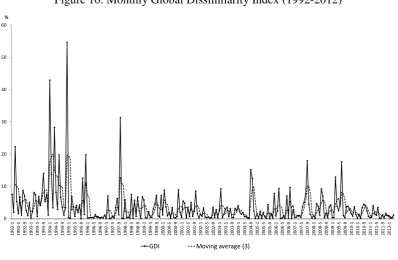
Figure 10. Monthly Global Dissimilarity Index (1992-2012)
Source: Author’s own elaboration with Banxico data.
0 10 20 30 40 50 60 1992 -1 1992 -5 1992 -9 1993 -1 1993 -5 1993 -9 1994 -1 1994 -5 1994 -9 1995 -1 1995 -5 1995 -9 1996 -1 1996 -5 1996 -9 1997 -1 1997 -5 1997 -9 1998 -1 1998 -5 1998 -9 1999 -1 1999 -5 1999 -9 2000 -1 2000 -5 2000 -9 2001 -1 2001 -5 2001 -9 2002 -1 2002 -5 2002 -9 2003 -1 2003 -5 2003 -9 2004 -1 2004 -5 2004 -9 2005 -1 2005 -5 2005 -9 2006 -1 2006 -5 2006 -9 2007 -1 2007 -5 2007 -9 2008 -1 2008 -5 2008 -9 2009 -1 2009 -5 2009 -9 2010 -1 2010 -5 2010 -9 2011 -1 2011 -5 2011 -9 2012 -1 %
Analyzing our empirical findings, we can see that the periods of high volatility in the
exchange rate show dissimilarities on the Hurst coefficient and α parameter. This mean
that they are far from their theoretical values (random walk H = 0.5 and α = 2). In the
graph, we can see a significant amount of values all of them corresponding to stress
periods. We want to emphasize that the quarterly and yearly index shows the same
[image:24.595.87.512.216.487.2]behavior.
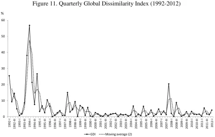
Figure 11. Quarterly Global Dissimilarity Index (1992-2012)
Source: Author’s own elaboration with Banxico data.
In the case of estimating the index on a yearly basis, the previously presented behavior
confirms the identification of thresholds on which the index peaks. In the years that
showed high volatility in the exchange rate, the index alert is triggered.
0 10 20 30 40 50 60 1992 -I 1992 -III 1993 -I 1993 -III 1994 -I 1994 -III 1995 -I 1995 -III 1996 -I 1996 -III 1997 -I 1997 -III 1998 -I 1998 -III 1999 -I 1999 -III 2000 -I 2000 -III 2001 -I 2001 -III 2002 -I 2002 -III 2003 -I 2003 -III 2004 -I 2004 -III 2005 -I 2005 -III 2006 -I 2006 -III 2007 -I 2007 -III 2008 -I 2008 -III 2009 -I 2009 -III 2010 -I 2010 -III 2011 -I 2011 -III 2012 -I %
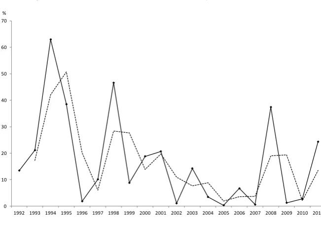
Figure 12. Annual Global Dissimilarity Index (1992-2011)
Source: Author’s own elaboration with Banxico data.
The proposed indicator is a useful tool that provides information on compliance of the
data with the assumptions of normality and white noise to the analyst; based on this
information every analyst should define their tolerance ranges and thresholds
dissimilarity bearable before modifying the methodologies used in the financial
analysis.
We calculate the IGD in three frequencies, monthly, quarterly and annually in
order to analyze the information dynamically. We recognize that the most robust index
version is the monthly, followed by the quarterly because more data improves the
estimation of the parameters. We recommend the use of this index in order to detect
heavy tails and dependence on the time series, our indicator will allow the analyst to
assess if his model is the best for the fitting of data, without having to force fit to the
normal case. Of course, the tolerance level of the dissimilarity measure depends on the
thresholds set by the analyst.
Although this analysis is only considering two major assumptions usually made
on financial series, they are of great importance in determining the best method for
analysis and prediction. In the case of the presence of self-similarity in series or
dependence on the time data it is possible to use the fractional Brownian motion.
0 10 20 30 40 50 60 70
1992 1993 1994 1995 1996 1997 1998 1999 2000 2001 2002 2003 2004 2005 2006 2007 2008 2009 2010 2011 %
Similarly to the case of the assumption of the absence of the normal series that can be
modeled by considering the use α-stable distributions to properly represent the presence
of heavy tails.
Our proposal is this is a first step towards improving the financial series
modeling, taking into account the characteristics of the series itself. Most of empirical
researchers are trying to look for information that allows them to leave as much as
possible the normal and independence assumptions that can be misleading, usually
incomplete. We have showed that the Hurst coefficient and the parameter α are useful as
early warning indicators of crises, when the relevant time series is the exchange rate,
because they provide a measure of market disparity compared to the theoretical values.
6. Conclusions
The existence of herd behavior, noise traders and complex microeconomic structures in
the different economies produce the existence of long memory and impulsiveness of
financial time series. These characteristics may lead to incorrect econometric analysis if
the independence and normality assumptions are not hold. The proposed methodology
gives the researchers a measurement of the accuracy of such assumptions.
This paper showed empirical evidence that the proposed index can be used as an
early warning alert for exchange rate crisis without making any assumption on the time
series probability distribution or the causes of the crisis. This is a major advantage in an
open economy that is exposed to many risk sources that works on some complex ways
that the economists have not fully understood.
The obtained results indicates that the independence and normality assumptions
made in the mainstream financial analysis are not always fulfilled, making them of little
use to decision making or prognosis, especially in high volatility crisis. The
quantification of the dissimilarity between the values of the time series parameters
respect to their theoretical values is important to validate the accuracy of the used
analysis tools, especially when the 5% confidence interval margin is reached faster than
References
Andersen, J. V., and D. Sornette (2004). Fearless versus fearful speculative financial
bubbles. Physica A: Statistical Mechanics and its Applications, Vol. 337, No. 3,
pp. 565-585.
Annis, A. A. and E. H. Lloyd (1976). The expected value of the adjusted rescaled Hurst
range of independent normal summands. Biometrika. Vol.63, No 1, pp.111-116.
Al-Anaswah, N., and B. Wilfling (2011). Identification of speculative bubbles using
state-space models with Markov-switching. Journal of Banking and Finance,
Vol. 35, No. 5, pp. 1073-1086.
Barany, E., M. Varela, B., I. Florescu, and I. Sengupta (2012). Detecting market crashes
by analysing long-memory effects using high-frequency data. Quantitative
Finance, Vol. 12, No. 4, pp. 623-634.
Barbulescu, A., and E. Bautu (2012). A hybrid approach for modeling financial time
series. Int. Arab. J. Inf. Technol., Vol. 9, No. 4, pp 327-335.
Belke, A., and G. Schnabl (2013). Four Generations of Global Imbalances. Review of
International Economics, Vol. 21, No. 1, pp. 1-5.
Belov, I. A. (2005). On the computation of the probability density function of α-stable
distributions. Mathematical Modelling and Analysis. Proceedings of the 10th
International Conference MMA 2005, Vol. 2, pp. 333-341.
Belov, I., A. Kabasinskas, and L. Sakalauskas (2006). A study of stable models of stock
markets. Information Technology and Control, Vol. 35, No.1, pp 34-56.
Beran, J. (1994), Statistics for Long-Memory Processes, Chapman and Hall. New York.
Cajueiro, D. O., and B. M. Tabak (2004). The Hurst exponent over time: testing the
assertion that emerging markets are becoming more efficient. Physica A:
Statistical Mechanics and its Applications. Vol. 336, No.3, pp. 521-537.
Cajueiro, D. O., and B. M. Tabak (2005). The rescaled variance statistic and the
determination of the Hurst exponent. Mathematics and Computers in Simulation,
Vol. 70, No. 3, pp. 172-179.
Cannon, M. J., D. B. Percival, D. C. Caccia, G. M. Raymond, and J. B. Bassingthwaighte (1997). Evaluating scaled windowed variance methods for
estimating the Hurst coefficient of time series. Physica A: Statistical Mechanics
and its Applications. Vol. 241, No. 3. pp. 606-626.
Cheung, Y. W. and S. L. Kon (1995). A search for long memory in international stock
market returns. Journal of International Money and Finance. Vol.14, No.4 pp.
597-615.
Chian, A. C. L. (2000). Nonlinear dynamics and chaos in macroeconomics.
International Journal of Theoretical and Applied Finance. Vol. 3, No.3, pp 601-611.
Comte, F., and E. Renault (1996). Long memory continuous time models. Journal of
Econometrics, Vol. 73, No.1, pp. 101-149.
Doukhan, P., G. Oppenheim, and M. S. Taqqu (2003). Theory and applications of long-range dependence (Eds.). Springer. New York.
DuMouchel, W. H. (1973). On the asymptotic normality of the maximum-likelihood
estimate when sampling from a stable distribution. The Annals of Statistics, Vol.
1, No. 5, pp. 948-957.
Fatum, R., J. Pedersen, and P. N. Sørensen (2013). The intraday effects of central bank
intervention on exchange rate spreads. Journal of International Money and
Finance, Vol. 33, 103-117.
Feldman, R., and M. Taqqu (1998). A practical guide to heavy tails: statistical techniques and applications. (Eds.). Springer, New York.
Frenkel, J. A., and H. G. Johnson (2013). The economics of exchange rates (Eds.). (Vol. 8). Routledge, London.
García-Ruiz, R. S., S. Cruz-Aké, and F. Venegas Martínez (2014). Una medida de
eficiencia de mercado: un enfoque de teoría de la información, Revista
Contaduría y Administración, Vol. 59, No. 4(247), pp. 137-166.
Glasserman, P. (2004). Monte Carlo Methods in Financial Engineering. Springer-Verlag. New York.
Granero, S., J. E. Trinidad-Segovia, and J. García-Pérez (2008). Some comments on
Hurst exponent and the long memory processes on capital markets. Physica A:
Statistical Mechanics and its Applications, Vol. 387, No. 22, pp. 5543-5551.
Greene, W. H. (2012). Econometric Analysis. Prentice Hall, 7th Edition. New Jersey,
USA.
Gürkaynak, R. S. (2008). Econometric Tests Of Asset Price Bubbles: Taking Stock.
Journal of Economic Surveys, Vol. 22, No.1, pp. 166-186.
Haas M. and C. Pigorsch (2007). Financial Economics, Fat-tailed Distributions.
Harvey, D. I., S. J. Leybourne, and R. Sollis (2013). Recursive Right-Tailed Unit Root
Tests for an Explosive Asset Price Bubble. Journal of Financial Econometrics,
forthcoming.
Hurst, H. E. (1951). The long term storage capacity of reservoirs, Transactions of the American Society of Civil Engineers, No. 1116, pp. 770-808.
Hurst, E. (1951). Long term storage capacity of reservoirs. Transactions on American
Society of Civil Engineering, No. 116, pp. 770-799.
Hurst, H. E., R. P. Black, and Y. M. Simaika (1965). Long-term storage: an
experimental study. Constable. London.
Jia, Z., M. Cui, and H. Li. (2012). Research on the relationship between the
multifractality and long memory of realized volatility in the SSECI. Physica A:
Statistical Mechanics and its Applications. Vol. 391, No.3, pp. 740-749.
Kaminsky, G. L. (2013). Varieties of Currency Crises. Annals of Economics and
Finance, Vol.14, No.3, pp. 1305-1340.
Kirchler, M., and J. Huber (2007). Fat tails and volatility clustering in experimental
asset markets. Journal of Economic Dynamics and Control, Vol. 31, No. 6, pp.
1844-1874.
Kolmogoroff, A. N. (1940). Wienersc He Spiralen Und einige andere in teressan te Kurv En im Hilb Ertsc hen Raum. C. R. (Dokl.) Acad. Sci. URSS (N.S.) Vol. 26, pp. 115-118.
Kosko, B. (2006). Noise. Penguin, New York, USA.
Koutsoyiannis, D. (2003). Climate change, the Hurst phenomenon, and hydrological
statistics, Hydrological Sciences Journal, Vol. 48, No.1, pp. 3-24.
Kulik, R. and P. Soulier (2011). The tail empirical process for long memory stochastic
volatility sequences. Stochastic Processes and their Applications, Vol. 121,
No.1, pp. 109-134.
Lamberton, D., and B. Lapeyre (2007). Introduction to stochastic calculus applied to finance. CRC Press.
Lim, K. P., R. D. Brooks, and J. H. Kim (2008). Financial crisis and stock market
efficiency: Empirical evidence from Asian countries. International Review of
Financial Analysis, Vol. 17, No. 3, pp. 571-591.
Lo, A. and A. C. MacKinlay (2002). A Non-Random Walk Down Wall Street. 5th Ed.
Princeton University Press.
Lux, T., and M. Marchesi (2000). Volatility clustering in financial markets: A
microsimulation of interacting agents. International Journal of Theoretical and
McCulloch, J. H. (1996a). Financial applications of stable distributions. In G. S. Maddala and C. R. Rao (Eds.), Handbook of Statistics, Volume 14. New York: North-Holland.
Machado, J. T., V. Kiryakova, and F. Mainardi (2011). Recent history of fractional
calculus. Communications in Nonlinear Science and Numerical Simulation,
Vol. 16, No. 3, pp. 1140-1153.
Mahalanobis, P. C. (1936). On the generalized distance in statistics. Proceedings of the
National Institute of Sciences of India Vol. 2, No 1, pp. 49–55.
Mandelbrot, B. (1963), The Variation of Certain Speculative Prices, The Journal of
Business. Vol. 36, No. 4, pp. 394-419.
Mandelbrot, B. (1965). “Forecasts of Future Prices, Unbiased Markets, and Martingale
Models”. The Journal of Business, University of Chicago Press, vol. 39, pp.
242-255.
Mandelbrot, B. B., and J. W. Van Ness (1968). Fractional Brownian motions, fractional
noises and applications. SIAM Review, Vol. 10, No. 4, pp 422-437.
Mandelbrot, B. (1971). “When Can Price be Arbitraged Efficiently? A Limit to the
Validity of the Random Walk and Martingale Models”. The Review of Economics and Statistics, Vol.53, No. 3, pp. 225-236.
Mandelbrot, B. (1997), Fractals and Scaling in Finance, Springer, EUA.
Mandelbrot, B. and J. W. van Ness. (1968), Fractional Brownian motions, fractional
noises and applications, SIAM Review. Vol. 10, No. 4, pp 422-437.
Mandelbrot, B. and H. Taylor (1967). On the Distribution of Stock Prices Differences.
Operations Research, Vol. 15, No. 6, pp 1057-1062.
McCulloch J. H. (1996) Handbook of Statistics, Elservier Science, Amsterdam, Chapter, Financial Applications of Stable Distributions.
McLachlan, G. (2004). Discriminant analysis and statistical pattern recognition (Vol. 544). John Wiley & Sons.
Meaning, J., and Zhu, F. (2011). The impact of recent central bank asset purchase
programmes. Bank of International Settlements Quarterly Review, Vol. 4, pp.
73-83.
Mensi, W., S. Hammoudeh, and S. M. Yoon (2014). Structural breaks and long memory in modeling and forecasting volatility of foreign exchange markets of oil exporters: The importance of scheduled and unscheduled news announcements.
Mielniczuk, J., and P. Wojdyllo (2007). Estimation of Hurst exponent revisited.
Computational Statistics and Data Analysis, Vol. 51, No. 9, pp. 4510-4525.
Mittnik, S., T. Doganoglu, and D. Chenyao (1999). Computing the probability density
function of the stable Paretian distribution. Mathematical and Computer
Modelling, Vol. 29, No. 10, pp. 235-240.
Mistrulli, P. E. (2011). Assessing financial contagion in the interbank market:
Maximum entropy versus observed interbank lending patterns. Journal of
Banking & Finance, Vol. 35, No. 5, pp. 1114-1127.
Neely, C. J. (2001). The practice of central bank intervention: looking under the hood.
Federal Reserve Bank of St. Louis Review, 83(May/June 2001).
Nolan, J. P. (1997). Numerical calculation of stable densities and distribution functions.
Communications in statistics. Stochastic models, Vol. 13, No 4, pp. 759-774.
Nolan J.P. (1999). Fitting Data and Assessing Goodness-of-fit with Stable Distributions. Department of Mathematics and Statistics, American University. Disponible en:
http://academic2.american.edu/~jpnolan/
Nolan, J. P. (2003). Modeling Financial distributions with stable distributions, Volume 1 of Handbooks in Finance, Chapter 3, pp. 105-130. Amsterdam: Elsevier.
Nolan J. P. (2005). Modeling financial data with stable distributions. Department of
Mathematics and Statistics, American University. Disponible en:
http://academic2.american.edu/~jpnolan/
Nolan J. P. (2009). Stable Distributions: Models for heavy tailed data. Department of
Mathematics and Statistics, American University. Disponible en:
http://academic2.american.edu/~jpnolan
Nourdin, I. (2012). Fractional Brownian Motion. In Selected Aspects of Fractional Brownian Motion (pp. 11-22). Springer Milan.
Oh, K. J., T. Y. Kim, and C. Kim (2006). An early warning system for detection of
financial crisis using financial market volatility. Expert Systems, Vol. 23, No.2,
pp. 83-98.
Oksendal, B. K. (2002), Stochastic Differential Equations: An Introduction with Applications, Springer, Berlin.
Parthasarathy, S. (2013). Long Range Dependence and Market Efficiency: Evidence
from the Indian Stock Market. Indian Journal of Finance. Vol. 7, No.1, pp.
17-25.
Revuz, D. and M. Yor (1999). Continuous Martingales and Brownian Motion, 2nd ed. New York: Springer-Verlag.
Rogers, L. C. G. (1997). Arbitrage with fractional Brownian motion. Mathematical
Finance, Vol. 7, No. 1, pp. 95-105.
Rostek, S., and R. Schöbel (2013). A note on the use of fractional Brownian motion for
financial modeling. Economic Modelling, Vol. 30, pp. 30-35.
Samorodnitsky, G. and M. Taqqu M. (1994). Stable Non-Gaussian Random Processes: Stochastic models with infinite variance. New York: Chapman and Hall.
Shrivastava, U., and A. Kapoor (2013). Long Memory in Rupee-Dollar Exchange Rate
Returns: A Robust Analysis. Asian Journal of Management, Vol. 4, No.3, pp
159-164.
Tankov, P. (2004). Financial modelling with jump processes. CRC Press. New York.
Taqqu, M. S. (2013). Benoît Mandelbrot and Fractional Brownian Motion. Statistical
Science, Vol. 28,No.1, pp. 131-134.
Thurner, S., J. D. Farmer, and J. Geanakoplos (2012). Leverage causes fat tails and
clustered volatility. Quantitative Finance, Vol. 12, No. 5, pp. 695-707.