A geometrical approach to structural change modeling

Munich Personal RePEc Archive

A geometrical approach to structural

change modeling

Stijepic, Denis

Fernuniversität in Hagen

9 October 2013

Online at

https://mpra.ub.uni-muenchen.de/55010/

A GEOMETRICAL APPROACH TO STRUCTURAL

CHANGE MODELING

Stijepic, Denis*

University of Hagen

This version: April 2014

Abstract: We propose a model for studying the dynamics of economic

structures. The model is based on qualitative information regarding structural

dynamics, in particular, (a) the information on the geometrical properties of

trajectories (and their domains) which are studied in structural change theory

and (b) the empirical information from stylized facts of structural change. We

show that structural change is path-dependent in this model and use this fact to

restrict the number of future structural change scenarios significantly. We

focus on labour-allocation-dynamics in a tree-sector-economy. However, our

approach can be applied to other types of structural change (e.g.

income-distribution-dynamics).

Keywords: structure, dynamics, qualitative, geometrical, simplex, path-dependency.

JEL-codes: C61, C69, D30, O14, O41.

1. INTRODUCTION

Many economic theories study the structure of the economy, e.g. the structure

of: GDP (break-down by types of expenditure/income), employment (labour

allocation across sectors), wages (wage distribution across agents) and income

(income distribution across households). Most of these theories study the

dynamics of this structure, i.e. structural change. In this paper we provide a

qualitative approach for studying structural change. We focus on the dynamics

of employment structure, i.e. dynamics of labour reallocation across sectors.

However, our approach can be applied to other structural change theories; see

Stijepic (2014a,b) for examples.

Recently, the dynamics of employment structure (in three-sector models) have

been analysed in many theoretical papers1. While these models feature specific

mathematical and economic assumptions, our qualitative model is very general

in this respect. It combines the information from empirical evidence (stylized

facts) and the information on the geometrical properties of typical trajectories

studied in structural change theory.2 We show that structural change is

path-dependent in our model and use this fact to reduce the number of future

structural change scenarios significantly.

The toolkit of the modern economist contains different tools for dynamic

analysis, e.g. vector auto regression, simulation and phase-diagram analysis.

Most of these tools combine theoretical and empirical information on the

subject of analysis for deriving some predictions regarding future dynamics or

policy responses. We do exactly the same. However, in contrast to many

quantitative and/or predominantly theoretical approaches we do not use

specific economic assumptions and, thus, do not follow specific economic

doctrines, but use the mathematical assumptions which are common to most

1

For example, Kongsamut et al. (2001), Meckl (2002), Ngai and Pissarides (2007), Acemoglu and Guerrieri (2008), Foellmi and Zweimueller (2008) and Buera and Kaboski (2009). 2

economic models. This idea results in a qualitative yet very general model of

structural change.

We approach as follows. First, we show that the dynamics of a three-sector

economy (agriculture, manufacturing, services) can be modelled on a

2-simplex; i.e. the 2-simplex is the domain of the structural change trajectory.

Second, we provide an economic interpretation of points and trajectories on

the 2-simplex. Third, we collect some information from widely-accepted

stylized facts of structural change and translate this information into dynamics

on the 2-simplex. Fourth, the structural change trajectories which arise in

structural change theory have some specific geometrical properties. In

particular, we use the fact that they are continuous and do not intersect

themselves (on the 2-simplex). Fifth, by combining the information from the

previous steps we obtain a qualitative meta-model of structural change. This

model implies that today’s structural change depends on past structural

change. That is, there is some sort of path-dependency in structural change.

Sixth, the path-dependency restricts the set of feasible future structural change

scenarios significantly. (For a summary of these scenarios see Section 9.) This

fact can be used in structural change predictions.

The rest of the paper is set up as follows. We show in Section 2 that structural

change in the three-sector-model can be depicted on a 2-simplex. In Section 3

we show how to interpret the points and trajectories on the 2-simplex. In

Section 4 we discuss briefly the stylized facts of labour allocation dynamics.

In Section 5 we present our model of structural change. In Section 6 we derive

the scenarios of structural change and show “path-dependency”. Section 7 is

devoted to a discussion of model assumptions. In Section 8 we show that most

structural change models assume implicitly continuous and

2. STRUCTURAL DYNAMICS AND STANDARD SIMPLEXES

Most aspects of the structure of an economy can be described by a set of

shares of an aggregate construct. This fact is illustrated in the following

examples. For a general discussion see Stijepic (2014a).

Example 1: If we are interested in the distribution of income across

households j =1,2,...h, we may study the shares of households j in aggregate

income y. That is, we study the system y_j /y, j=1,2,...h, where y_j is the

income of household j.

Example 2: Labour allocation across sectors. Assume that E is some measure

of aggregate employment (e.g. the number of hours worked in the whole

economy). Furthermore, let E_i denote the employment in sector i (e.g. hours

worked in sector i). The literature on labour allocation (cited in Section 1)

studies the dynamics of the system _i:= E_i/E, i=1,2,...n, where n is the

number of sectors and _i is the employment share of sector i.

We focus on Example 2. There are two facts which allow us to model labour

allocation (Example 2) on a standard simplex: (I) Standard structural change

literature (see Section 1) assumes that ₁+₂+..._n =1. That is, all labour available is employed in sectors i=1,2,...n or, equivalently, E is the aggregate

of sectors i=1,...n, i.e. E:=E₁+E₂ +...E_n. This definition is not crucial for any result, since, if E≠E₁ +...E_n, we can always define an auxiliary variable

1 +

n

E such that E=E₁+...E_n+E_n+1 and study the dynamics of the system

E E_i i:= /

 , i=1,...n+1. (II) The definitions _i:=E_i/E, i=1,...n, and

n E E

These facts reduce the set of all feasible _i drastically: the _i are located on a

standard simplex of dimension (n-1).3 Let ∆_(n−1) denote this simplex; thus,

} 1 ... ;

,... 1 , 0 : ) ,... , {(

: _{1 2 1 2}

) 1

( = ∈ ≥ = + + =

∆ _n−   _n n _i i n   _n

R .

In the main part of the paper we will study a lower-dimensional case of

Example 2, as defined in the following assumption.

ASSUMPTION 1: a) We study an economy divided into three sectors:

agriculture (a), manufacturing (m) and services (s). b) _i denotes the share of

labour devoted to sector i, i=a,m,s. c) The employment shares i satisfy the

following relations:

(1) _a+_m+_s =1

(2) 0≤_i ≤1 for i=a,m,s.

According to the discussion above, the employment shares of the economy

defined in Assumption 1 are located on a subset of a two-dimensional standard

simplex (∆₂), where ∆₂ is given by the following definition:

(3) : {( , , ) 3: 0, , , ; 1}

2 = ∈ ≥ = + + =

∆ _a _m _s R _i i a m s _a _m _s

where (_a,_m,_s) is a vector of Cartesian coordinates indicating the labour

allocation and R is the set of real numbers.

In the remaining part of this section we recapitulate some standard geometrical

concepts for the analysis of the system defined in Assumption 1.

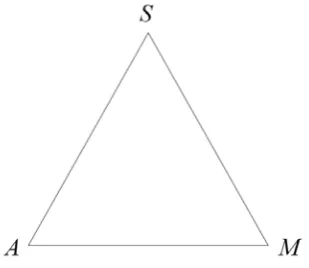
The simplex ∆₂ is a triangle. In Figure 1 we depict ∆₂ in a three-dimensional

Cartesian coordinate system with the coordinates (_a,_m,_s).

3

Figure 1: The simplex ∆₂ in the Cartesian coordinate system (a,m,s).

The vertices (A, M, S)and the origin (O) of the coordinate system in Figure 1

can be expressed in Cartesian coordinates (a,m,s) as follows:

(4) A:=(1,0,0)

(5) M :=(0,1,0)

(6) S:=(0,0,1)

(7) O:=(0,0,0)

Since the depiction in Figure 1 is inconvenient and unnecessary, we depict,

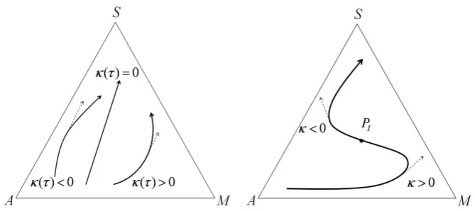
henceforth, ∆₂ in the plane, as shown in Figure 2.

Imagine a trajectory τ on ∆₂ describing a movement from vertex A to vertex

S, cf. Figure 3. To abbreviate discussion, we define here the concept of

“signed curvature” (κ) of a trajectory in a very simple and somewhat

restrictive way; for a rigorous mathematical definition see any book on

introductory differential geometry. We say that the signed curvature of τ is

uniformly positive (κ(τ)>0), if the tangential vector is always on the

right-hand-side of τ ; i.e. τ describes a counter-clockwise movement. The signed

curvature of τ is uniformly negative (κ(τ)<0), if the tangential vector is

always on the left-hand-side of τ ; i.e. the movement described by τ is

clockwise. If the curvature of τ is uniformly zero (κ(τ)=0), then τ is an

oriented line-segment. These definitions imply that, if the curvature of τ is

“uniform”, there are no inflection points on τ . See Figure 3.

Figure 3: Curvature of trajectories on ∆₂ and an inflection pointP_I .

3. INTERPRETATION OF POINTS AND TRAJECTORIES ON THE

2-SIMPLEX

In this section we elaborate the interpretation of points and vectors/trajectories

Remark 1: First, we turn to the interpretation of points on ∆₂. (4)-(6) imply

that at the vertices A, M and S all labour is employed in agriculture,

manufacturing and services, respectively; cf. Figure 1. Thus, we define:

DEFINITION 1: a) An economy situated in vertex A of ∆₂ is named “pure

agricultural economy”. b) An economy situated in vertex M of ∆₂ is named

“pure manufacturing economy”. c) An economy situated in vertex S of ∆₂ is

named “pure services economy”.

LEMMA 1: a) All points on the MS-edge of ∆₂ feature _a =0. b) All points

on the SA-edge of ∆₂ feature _m =0. c) All points on the AM -edge of ∆₂

feature _s =0. See also Figure 2.

PROOF: This property of the standard 2-simplex is well-known. For a proof

see APPENDIX A. 

Remark 2: Thus, an economy situated on the MS-edge of ∆₂ or moving

along this edge does not employ any labour in the agricultural sector.

Analogously, on the SA-edge labour is not employed in the manufacturing

sector and on the AM-edge labour is not employed in the services sector.

Remark 3: The following three lemmas show how a movement

(directional/tangential vector or trajectory) on ∆₂ can be interpreted in terms

of sectoral employment share dynamics.

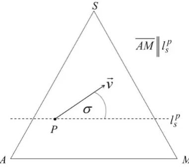
LEMMA 2: Assume that (I) P is an arbitrary point in the interior of ∆₂, (II)

v is the directional vector associated with point P indicating the direction of

movement from point P along ∆₂, (III) p s

parallel to the AM -edge of ∆₂ and (V) σ is the angle between p s

l and v (in

point P); cf. Figure 4. Under these assumptions the following is true:

a) If 0°<σ <180°, the movement from P in direction indicated by v is

associated with an increase in _s.

b) If 180°<σ <360°, the movement from P in direction indicated by v is

associated with a decrease in s.

c) If σ =180° or if σ =0°, the movement from P in direction indicated by v

is not associated with a change in _s.

PROOF: This property of the standard simplex is well-known. For a proof see

APPENDIX A. 

Figure 4: A directional vector on ∆₂ in relation to an AM-parallel ( p s l ).

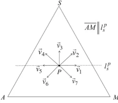
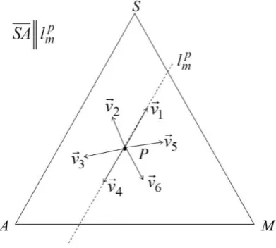
Remark 4: Figure 5 illustrates Lemma 2. The vectors v₁ and v₅ are parallel to

AM. Thus, a movement along these vectors is not associated with a change in

the service-share (_s). Along vectors v₂, v₃ and v₄ the service-share

increases. Along vectors v₆ and v₇ the service-share decreases. Overall, we

is associated with an increase/decrease in _s: if all tangential vectors on this

segment have an angle between 0 and 180 degrees to the edge AM , we know

that s increases steadily along this trajectory segment.

Figure 5: Representative vectors regarding _s-changes.

LEMMA 3: Assume that (I) P is an arbitrary point in the interior of ∆₂, (II)

v is the directional vector associated with point P indicating the direction of

movement from point P along ∆₂, (III) p m

l is a line going through P, (IV) p m l is

parallel to the SA-edge of ∆₂ and (V) µ is the angle between p m

l and v (in

point P); cf. Figure 6. Under these assumptions the following is true:

a) If 0°<µ <180°, the movement from P in direction indicated by v is

associated with a decrease in m.

b) If 180°<µ<360°, the movement from P in direction indicated by v is

associated with an increase in _m.

c) If µ =180° or if µ =0°, the movement from P in direction indicated by v

is not associated with a change in _m.

Figure 6: A directional vector on ∆₂ in relation to a SA-parallel ( p m l ).

Remark 5: Figure 7 illustrates Lemma 3: movement along vectors v₁ and v₄

is not associated with a change in the manufacturing-share (_m); _m declines

along vectors v₂ and v₃; _m increases along vectors v₅ and v₆.

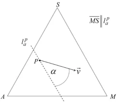
LEMMA 4: Assume that (I) P is an arbitrary point in the interior of ∆₂, (II)

v is the vector associated with point P indicating the direction of movement

from point P along ∆₂, (III) p a

l is a line going through P, (IV) p a

l is parallel to

the MS-edge of ∆₂ and (V) α is the angle between p a

l and v (in point P); cf.

Figure 8. Under these assumptions the following is true:

a) If 0°<α <180°, the movement from P in direction indicated by v is

associated with a decrease in _a.

b) If 180°<α <360°, the movement from P in direction indicated by v is

associated with an increase in a.

c) If α =180° or if α =0°, the movement from P in direction indicated by v

is not associated with a change in _a.

PROOF: Analogous to the Proof of Lemma 2. 

Figure 8: A directional vector on ∆₂ in relation to a MS-parallel ( p a l ).

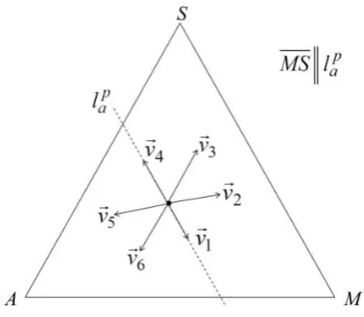
Remark 6: Figure 9 illustrates Lemma 4: movement along vectors v₁ and v₄

is not associated with a change in the agriculture-share (_a); _a declines

along vectors v₂ and v₃; a increases along vectors v5 

Figure 9: Representative vectors regarding a-changes.

Remark 7: Lemmas 2-4 show how to interpret a movement (a directional

vector or trajectory) on ∆₂. The angle set (α,µ,σ) associated with a

directional vector gives us all the necessary information about the structural

change associated with the movement along the vector.

Remark 8: The interpretation of directional vectors derived in this section

allows us to interpret trajectories on ∆₂ directly, i.e. without analysis of

three-dimensional Cartesian coordinates of trajectories. That is, we can analyse

structural change as dynamics of a system on a bounded subset of the plane.

This allows us to benefit from the nice properties of such systems mentioned

in Section 1; cf., e.g., Guckenheimer and Holmes (1990), p.42f.

4. STYLIZED FACTS OF STRUCTURAL CHANGE

Theories of long-run labour reallocation across sectors have a long tradition in

economics. Some classical contributions are, for example: Clark (1940),

Baumol (1967) and Kuznets (1969). For a detailed review of structural change

Teixeira (2008). Most studies focus on a three-sector framework (agriculture,

manufacturing, services). Some newer empirical evidence on labour dynamics

in this framework is provided by Maddison (1989, 1995a,b, 2007), Kongsamut

et al. (2001) and Raiser et al. (2004). Some of this evidence is depicted in

APPENDIX F. Throughout the paper we will use the US-dynamics as an

example (cf. Figure 10).

Figure 10: Past structural change dynamics in the USA (standard diagram).

Data source: Maddison, Angus (2007): Contours of the World Economy I-2030 AD, Essays in Macro-economic History, Oxford University-Press, New York, p.384

We use the following widely-accepted stylized facts in our model.

Stylized Fact 1: At early stages of development the economy is dominated by

agriculture (“agricultural economy”). This is one of the best known facts of

development economics. For evidence see any contribution on structural

change, e.g. Maddison (1989, 1995a,b, 2007), Kongsamut et al. (2001) and

Raiser et al. (2004). Figure 10 implies that 70% of labour has been employed

Stylized Fact 2: At later stages of development the economy is dominated by

services (“services economy”). “Later stages of development” refers here to

industrialized countries (e.g. OECD core-countries). For evidence on high

service-share in industrialized countries see e.g.: Schettkat and Yocarini

(2006), Maddison (1989, 1995a,b, 2007) and Raiser et al. (2004); see also the

figures in APPENDIX F. For example, Figure 10 implies that nearly 80% of

labour has been employed in the services sector in 2003 in the USA.

Stylized Fact 3 (Long-run trend): The employment share of agriculture

declines over the development process. See also Kongsamut et al. (2001). This

stylized fact is an implication of Stylized Facts 1 and 2. For evidence see e.g.:

the regression results presented by Kongsamut et al. (1997, 2001), the

evidence presented by Maddison (1989, 1995a,b, 2007), Figure 10 and the

figures in APPENDIX F.

Stylized Fact 4 (Long-run trend): The employment share of services grows

over the development process. See also Kongsamut et al. (2001). This stylized

fact is an implication of Stylized Facts 1 and 2. For evidence see e.g.: the

regression results presented by Kongsamut et al. (1997, 2001), the evidence

presented by Maddison (1989, 1995a,b, 2007), Figure 10 and the figures in

APPENDIX F.

These well-known and widely accepted stylized facts are necessary for our

results. For the sake of completeness, we add a further stylized fact, which is

not necessary for our results.

Stylized Fact 5 (optional): The employment share of manufacturing grows at

early stages of development (“industrialization”) and declines at later stages

of development (“tertiarisation”). This stylized fact implies that the curve

which describes the dynamics of manufacturing sector employment is

concave; cf. Figure 10. This result has been emphasized by Ngai and

Pissarides (2007). It may be questioned whether this stylized fact applies to all

countries. Furthermore, we are dealing here with long-run growth modelling;

could not find any trend in manufacturing employment share; therefore, they

postulate the following stylized fact:

Stylized Fact 5’ (optional): The manufacturing employment share is

“constant” over the development process.

Our model covers all these cases (Fact 5 and 5’): our results are consistent

with a inclining, declining, constant, concave or convex manufacturing-share

(curve).

Note that the dynamics depicted in the standard diagram (Figure 10) can be

translated into dynamics on ∆₂ by using Lemmas 1-4; see also APPENDIX B.

5. A QUALITATIVE MODEL OF STRUCTURAL CHANGE

In this section we define a qualitative model which satisfies the stylized facts

postulated in Section 4. In the next section we use this model to elaborate

scenarios of future structural change.

ASSUMPTION 2: a) The dynamics of the sector structure (_a,_m,_s) on ∆₂

are described by the curve φ(t), t<t<t, t∈R, where: φ(t) is a coordinate

vector determining the position of the economy on ∆₂ at time t; R is the set of

Real numbers. b) φ(t)∈∆₂ for t<t <t . c) φ(t) is continuous (in t) on ∆₂ for

t t t < < .

DEFINITION 2: a) φ(t₀)=:P₀ and φ(t_T)=:P_T, where t <t₀ <t_T <t .

b) τ :={φ(t)∈∆₂ :t<t <t} is the trajectory on ∆₂ describing the dynamics

of sector structure for t <t <t .

c) τ_0T :={φ(t)∈∆₂ :t₀ ≤t ≤t_T} is the segment of trajectory τ connecting the

points P and ₀ P_T.

e) τ₀₋ :={φ(t)∈∆₂ :t<t₀} denotes the τ -segment preceding point P . ₀

f)



T t t t T t ≤ ≤ = 0 ) ( : ]

[τ₀ φ is the set of all points covered by trajectory-segment τ_0T.

Remark 9: (i) Implicitly, we assume here some economic model which

generates a continuous trajectory (τ ) on ∆₂, cf. Assumption 2 and Definition

2b. For discussion and examples of mathematical and economic models which

generate continuous trajectories of structural change see Section 8. (ii) We

partition the trajectory τ in segments, cf. Definition 2c-e. (iii) We assume the

existence of a continuous trajectory (cf. Assumption 2c), since we analyse

long-run structural change. It is hard to imagine that

sector-employment-shares jump (i.e. change non-marginally) at some point in time, since (a)

changes in sector-employment-shares require labour reallocation across

sectors and (b) significant numbers of workers cannot be reallocated instantly.

ASSUMPTION 3: Let the Cartesian coordinates of points P₀ and P_T (cf.

Definition 2a) be given as follows: P0 =(0a,0m,0s) and T ( )

T s T m T

a, ,

P =    . The

trajectory segment τ_0T satisfies the following qualitative requirements:

a) P is relatively close to vertex A, i.e. ₀ 0a >1/2; cf. Figure 2.

b) P_T is relatively close to vertex S, i.e. T >1/2 s

 ; cf. Figure 2.

c) τ_0T has uniform signed curvature (κ(τ0T)>0 or κ(τ0T)<0 or κ(τ0T)=0),

i.e. τ_0T has no inflection points; cf. Section 2 and Figure 3.

d) The economy approaches P_T monotonously along τ_0T; i.e. all tangential

vectors on τ_0T satisfy the following (vector-angle-)conditions: 0°≤σ ≤180°

Remark 10: Remember that Definition 2a/c implies that trajectory-segment

T

0

τ describes a movement from point P₀ to point P_T; the economy is in P₀ at

time t₀ and in P_T at time t_T. Thus, Assumption 3 can be explained as follows:

a) Assumption 3a is due to Stylized Fact 1. Stylized Fact 1 states that

agriculture is dominant at the beginning of the development process (t0); cf.

Section 4. Assumption 3a implies that more than 50% of labour is employed in

the agricultural sector at t₀; thus, Stylized Fact 1 is satisfied. Note that Lemma

4b implies: the closer a point to vertex A, the greater the employment share of

agriculture (_a); cf. Remark 6.

b) Assumption 3b is due to Stylized Fact 2. Stylized Fact 2 states that the

services sector is dominant at later stages of development (t_T); cf. Section 4.

Assumption 3b implies that more than 50% of labour is employed in the

services sector at tT; thus, Stylized Fact 2 is satisfied. Note that Lemma 2a

implies: the closer a point to vertex S, the greater the employment share of

services (_s); cf. Remark 4. We discuss Assumption 3b in Section 7.1 as well.

c) Assumption 3c follows from our growth-theoretical approach to structural

change; cf. Section 4. We are interested in long-run trends not fluctuations.

Thus, in general, the assumption of a linear trajectory (κ(τ0T)=0) is

sufficient for our analysis; for example, the stylized facts and the model

elaborated by Kongsamut et al. (2001) imply a linear trajectory of structural

change on ∆₂. We allow for uniformly positive (κ(τ_0T)>0) and uniformly

negative (κ(τ_0T)<0) signed curvature of τ_0T for reasons of generality. If τ_0T

had one or many inflection points in reality, its trend could be approximated

by a trajectory with uniform signed curvature; see also the discussion of

Stylized Fact 5 in Section 4. Furthermore, our results remain valid, if there are

inflection points, provided that τ_0T does not feature strong fluctuations; we

d) Assumption 3d is due to Stylized Facts 3 and 4. Stylized Facts 3 and 4 refer

to long-run trends and state that services employment share (_s) increases

over the development process and agricultural employment share (a)

decreases over the development process. Assumption 3d (and Assumption

3a/b) implies that _s increases monotonously over time (0°≤σ ≤180°, cf.

Lemma 2 and Figure 4) and _a decreases monotonously over time

° ≤ ≤

° 180

0

( α , cf. Lemma 4 and Figure 8). The assumption of monotonous

dynamics is due to the fact that we analyse here long-run trends; cf. Remark

10c. In Section 7 we show that this assumption is not necessary for our results.

LEMMA 5: If Assumptions 1-3 are satisfied, the dynamics described by

trajectory-segment τ_0T are consistent with Stylized Facts 1-4 (cf. Section 4).

PROOF: For a proof of Lemma 5, see Remark 10a/b/d. 

ASSUMPTION 4: The trajectory τ does not intersect itself. In particular,

] [ ) (t τ_0T

φ ∉ for t>tT (cf. Definition 2f).

Remark 11: Assumption 4 implies that the economy never returns to a state in

which it has been previously. This assumption is widespread in structural

change analysis and in mathematical literature. We discuss it in Section 8.

Remark 12: Assumption 4 does not allow for closed trajectories. A closed

trajectory (or: closed orbit) in the plane is a Jordan curve. For example, the

circle is a Jordan curve. The economy moving along such a closed trajectory

repeats the cycle (infinitely) many times. Thus, if an economy satisfies

Assumption 1-3 and moves along a closed trajectory, at some point in time

T t

t> the economy enters the set [τ₀T] and moves along it (from point P0 to

also APPENDIX C and D. On closed trajectories, see any introductory book

on differential equation systems.

DEFINITION 3: a) An economy situated in point ( , , ps)

p m p a

P=    at time

T D t

t > “has undergone a process of relative deindustrialization since t ”, if _T

there exists a point T _T

s T m T a T , ,

P₀ =(0 0 0 )∈τ₀ such that T s p s

0



 = and

. 0T m p m 

 < b) An economy situated in point ( , , p)

s p m p a

P=    at time t_I >t_T

“has undergone a process of relative industrialization since t ”, if there _T

exists a point T _T

s T m T a T , ,

P₀ =(0 0 0 )∈τ₀ such that T s p s

0



 = and T

m p m

0

  > .

Remark 13: a) If we want to know whether an economy at time t_D >t_T “has

undergone a process of relative deindustrialization since t_T”, we have to do

the following. First, find data on services employment share ( p s

 ) at time

T D t

t > . Second, find a data-point (P0_T) in the past – exactly speaking, in the

period [t₀,t_T] – which satisfies T s p s

0



 = , i.e. the services share associated

with P_0T is equal to the services share at tD. Third, compare the

manufacturing employment share associated with P0_T to the manufacturing

employment share at t_D. If 0T

m p m 

 < , then the economy “has undergone a

process of relative deindustrialization since t_T”. b) Definition 3b implies that

the concept of “relative industrialization” is antipodal to the concept of

“relative deindustrialization”: while “relative deindustrialization” implies that

today’s manufacturing-share is relatively small, “relative industrialization”

implies that today’s manufacturing-share is relatively great. c) Remarks 13a/b

imply that the concept of “relative (de)industrialization” (Definition 3) is

based on comparing the today’s share to the

“comparable” to today’s situation if the service-share in the past situation is

equal to today’s service-share.

DEFINITION 4: Let the Cartesian coordinates of points P₀ and P_T (cf.

Definition 2a) be given as follows: P0 =(0a,0m,0s) and ( ) T s T m T a T , , P =    .

Furthermore, let the Cartesian coordinates of a point P_0T∈[τ_0T] be given as

follows: 0 ( 0 0 0 ) T s T m T a T , ,

P =    . We define the following partitions of ∆₂ (cf.

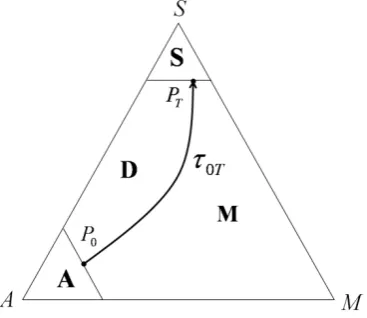
Figure 11):

(8) A:={(a,m,s)∈∆2 :a ≥0a}

(9) : {( , , ) 2 : }

T s s s

m

a    

 ∈∆ ≥

=

S

(10) D:=L∩(∆₂\(A∪S))

(11) M:=∆₂\(A∪S∪D∪[τ_0T])

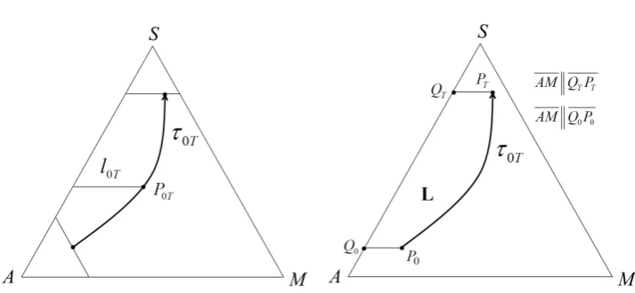
where L is given by 0 : {( , , ) 2 : 0 , 0 }

T m m T s s s m a T

l =    ∈∆  =  < and

]} [ :

{

: 0 0 0

p T T T P τ

l ∈

=

L .

Figure 11: A partitioning of ∆₂ according to Definition 4.

Remark 14: a) For an explanation of partitions A and S see (Proof of) Lemma

follow from Definition 4 and Lemmas 4 and 2. b) The explanation of partition

D is a little bit more complicated. Imagine an arbitrary point

) ( 0 0 0 0 T s T m T a T , ,

P =    on the trajectory τ_0T. The set of all points (_a,_m,_s) on

2

∆ which satisfy T

s s

0



 = and T

m m

0



 < is given by {(_a,_m,_s)∈∆₂ :

T T m m T s

s , l0

0 0

}≡

<

=  

 . The basic knowledge of calculus implies that (cf.

Figure 12): l_0T is a line-segment on ∆2; l0T is parallel to the AM -edge of

2

∆ (cf. Lemma 2c and Figures 4); l_0T is bounded on the right-hand side by

the point P0_T and on the left-hand side by the AS-edge of ∆2 (cf. Lemma

3a/c). Thus, l0_T is the set of all points on ∆2 which are situated on the

left-hand side of point P0_T; cf. Figure 12. If we do this procedure with every point

on τ_0T and join all the line-segments l_0T which are created by this procedure,

we obtain the set L:={l0T :P0T ∈[τ0T]}; cf. Figure 12. D is given by

2 ( :=L∩ ∆

D \(A∪S)), cf. Definition 4. For economic interpretation of

partition D see (Proof of) Lemma 6. c) The partition M is the part of ∆₂ which

is not assigned to the other partitions (A, S, D, [τ_0T]). It contains all the points

which are on the right-hand side of τ_0T. The proof of this fact is analogous to

the proof in Remark 14b.

DEFINITION 5: a) In an “agricultural economy” the greatest share of

labour is employed in the agricultural sector, i.e. _a >1/2. b) In a

“manufacturing economy” the greatest share of labour is employed in the

manufacturing sector, i.e. m >1/2. c) In a “services economy” the greatest

share of labour is employed in the services sector, i.e. s >1/2.

LEMMA 6: a) An economy situated in partition A is an agricultural economy

(cf. Definition 5a). b) An economy situated in partition S is a “services

economy” (cf. Definition 5c). c) An economy situated in partition D “has

undergone a process of relative deindustrialization since t_T” (cf. Definition

3a). d) Partition M contains all the points which satisfy Definition 3b

(“relative industrialization”).

PROOF: a) Definition 4 and Assumption 3a imply that all points in partition

A satisfy the following inequality: a ≥0a >1/2. This fact implies Lemma

6a; cf. Definition 5a. b) Definition 4 and Assumption 3b imply that all points

in S satisfy the following condition: T 1/2 s s ≥ >

 . This fact implies Lemma

6b; cf. Definition 5c. c) The definition of l0_T (cf. Definition 4) implies that all

points which belong to l_0T satisfy Definition 3a, i.e. if an economy is situated

on l0_T, then the economy “has undergone a process of relative

deindustrialization since t_T”. (Note that l0_T exists only for t>tT; cf.

Definition 4). Definition 4 implies that L consists of such line-segments, i.e.

line-segments which satisfy Definition 3a. Thus, L satisfies Definition 3a as

well. D is a subset of L. Thus, D satisfies Definition 3a. That is, an economy

situated in partition D “has undergone a process of relative deindustrialization

since t_T”; cf. Definition 3a, which proves Lemma 6c. d) The proof of Lemma

6d is analogous to the proof of Lemma 6c. Note, however, that M does not

only contain points which satisfy Definition 3b but also points which do not

they are not “comparable” (cf. Remark 13c). We omit the discussion of this

fact, since it has no relevance for our results. 

LEMMA 7: Assume an economy which satisfies Assumptions 1-4. Let this

economy be situated in partition S at time t , i.e. S φ(tS)∈S, where tT ≤tS <t .

If this economy leaves S, then it must enter D or M. That is: if φ(t)∉S for

x S t t

t < < , then either φ(t)∈D for t_S <t<t_D≤t_x or φ(t)∈M for

x M S t t t

t < < ≤ , where tx >tS, tD >tS and tM >tS are points in time.

PROOF: Note that Definition 4 implies that S is a closed set; thus, (i) the

boundary between S and M belongs to S and (ii) the boundary between S and

D belongs to S; cf. Figure 11. The proof of Lemma 7 can be divided into the

following parts.

LEMMA 8: If φ(t)∉S, then φ(t)∈A∪M∪D∪int([τ0T]). PROOF:

Definition 4, which defines a partitioning of ∆₂, and Assumption 2b imply

Lemma 8. See also Definition 2f. ◊

In the following we discuss which of the partitions (A, M, D, int([τ0T])) the

economy can enter at the instant at which it leaves S.

LEMMA 9: Let Z denote a partition of ∆2, i.e. Z∈{A,M,D,S,int([τ0T])}.

Assume that Z and S are separated. Then the following is true: if φ(t_y)∈S

then φ(t_z)∉Z for t_z →t_y, where t_z >t_y. PROOF: Two sets X⊂∆₂ and Y

2

∆

⊂ are separated if X*∩Y=X∩Y*=∅, where X* is the closure of X and

Y* is the closure of Y; see e.g. Flegg (1974), p.163f. Thus, Lemma 9 is

implied by the fact that φ(t) is continuous (cf. Assumption 2c) and S and Z

are separated. The economy cannot “jump” from S to Z, since a “jump”

contradicts the continuity assumption. ◊

LEMMA 10: Partitions S and A are separated. PROOF: Lemma 9 is implied

by Definition 4 and Assumption 3a/b. In particular, the fact that Assumption

implies that partitions S and A are separated by a non-empty set

) ]) int([

(D∪ τ_0T ∪M ; cf. Definition 4 and Figure 11. This vague statement

can be specified as follows. If 0a >1/2 and >1/2 T

s

 (cf. Assumptions 3a/b)

S and A are separated, as shown in the following proof. If S and A are not

separated then there must exist a point P=(l_ap,l_mp,l_sp)∈∆₂ which satisfies (i)

∈

P A* and P∈S or (ii) P∈A and P∈S*; cf. Proof of Lemma 9. (8) and (9)

imply that in the cases (i) and (ii) the following is true: 0

a p a l

l ≥ and T

s p s l l ≥ .

Thus, since we assume 0a >1/2 and >1/2 T

s

 , the following is true: pa >1/2

and ps >1/2 and, thus, + >1 p s p a l

 . This contradicts (1). Thus, S and A are

separated if 0a >1/2 and >1/2 T

s

 . ◊

LEMMA 11: In general, (i) S and M are not separated and (ii) S and D are

not separated. PROOF: Lemma 11 is implied by Definition 4 and Assumption

3; cf. Figure 11. For the case where S is separated from M and D see the

discussion at the end of this proof. ◊

LEMMA 12: φ(t)∉int([τ_0T]) for t >t_S. PROOF: Lemma 12 is implied by the

fact that t_S ≥t_T (as assumed in Lemma 7) and by Assumption 4. ◊

LEMMA 13: Assume that S is not separated from M and/or D. Then the

following is true: if φ(t_S)∈S and φ(t_z)∉S then φ(t_z)∈M or φ(t_z)∈D for

S z t

t → , where t_z >t_S. PROOF: This lemma is implied by Lemmas 8-12. ◊

Lemma 13 completes the proof of Lemma 7. Note that, if S is separated from

M and D, the economy cannot leave S (due to Assumption 2c) and, thus, stays

in S. In this case the premise of Lemma 7 (“...if φ(t)∉S for tS <t<tx...”) is

not satisfied. That is, this case is not relevant for Lemma 7. Furthermore, note

that Lemma 7 would hold, even if we allowed that τ is a closed trajectory (cf.

6. MODELL-PREDICTIONS OF STRUCTURAL CHANGE

We will assume now that t₀ corresponds to a point in time in the early history

of an industrialized country (e.g. the year 1820 in the history of the USA; cf.

Figure 10). Furthermore, we assume that t_T corresponds to now. Thus, the

trajectory-segment τ_0T corresponds to the past structural change (in the USA)

and the trajectory-segment τT₊ corresponds to the future structural change (in

the USA). We translate now the properties of τ_T+ into structural change

scenarios. First, we show that there are three scenarios of future development.

Then, we discuss how these scenarios can be continued.

LEMMA 14: The economy which satisfies Assumptions 1-4 is situated in

partition S at time t_T.

PROOF: Definition 2a implies that the economy is in point P_T at time t_T.

Definition 4 implies that the point P_T is located in partition S. 

THEOREM 1: Assume an economy which satisfies Assumptions 1-4. Let this

economy be situated in partition S at time t=t_T, i.e. φ(t_T)∈S (cf. Lemma

14). There are only three alternative scenarios regarding the development of

this economy in the future (t >t_T):

Scenario I: The economy stays in S for t >t_T, i.e.

φ

Figure 13.

Scenario II: At some point in time tSD >tT the economy departs from S and

enters D. That is,

φ

φ

where t_x >t_SD is some point in time. See also Figure 14.

Scenario III: At some point in time tSM >tT the economy departs from S and

enters M. That is,

φ

φ

PROOF: The economy being in S can stay in S forever. This outcome is

possible if, for example, the economy converges to a fixed point in S. If the

economy does not stay in S, i.e. if the economy leaves S, the economy must

enter D or M; cf. Lemma 7. Note that Definition 4 implies that S is a closed

set; thus, (i) the boundary between S and M belongs to S and (ii) the boundary

between S and D belongs to S. 

Figure 13: Scenario I.

Figure 15: Scenario III.

Remark 15: Of course, when the economy is in D (Scenario II) or in M

(Scenario III), it can move further to A or go back to S. These “secondary

steps” (sub-scenarios) will be discussed later.

COROLLARY 1 (Economic Interpretation of Theorem 1): Assume an

economy which (a) satisfies Assumptions 1-4 and (b) is dominated by the

services sector today. Then, there are only three alternative scenarios

regarding future development of this economy. (I) The economy remains a

“services economy” forever (cf. Definition 5c). (II) At some future point in

time the economy starts a process of “relative deindustrialization” (cf.

Definition 3a). (III) At some future point in time the economy starts a process

of “relative industrialization” (cf. Definition 3b).

PROOF: a) Theorem 1 postulates that in Scenario I the economy stays in S

forever. Lemma 6b shows that the economy situated in S is a services

economy. b) Theorem 1 postulates that in Scenario II the economy enters D.

Lemma 6c implies that the economy situated in partition D “has undergone a

process of relative deindustrialization since t_T” (cf. Definition 3a). c) Theorem

the economy situated in partition M “has undergone a process of relative

industrialization since t_T” (cf. Definition 3b). 

Remark 16: a) In Scenario I the service-share (_s) does not fall below its

today’s level, i.e. _s ≥T_s for t>t_T. b) Scenario I implies that there is some

fixed point or limit cycle in S; cf. Stijepic (2014a), “Theorem 1”, on the

limit-properties of trajectories satisfying Assumptions 1-4. c) The structural change

models discussed in Section 1 predict Scenario I (fixed point).

Remark 17: Scenario II implies that at some future point in time the

service-share (_s) starts shrinking (cf. Definition 4, Lemma 2b and Figure 14) while

the manufacturing sector remains below “comparable” past levels; cf.

Definition 3a and Remark 13c.

Remark 18: Scenario III implies that at some future point in time the

service-share (_s) starts shrinking (cf. Definition 4, Lemma 2b and Figure 15) while

the manufacturing sector remains above “comparable” past levels; cf.

Definition 3b and Remark 13c.

Remark 19: Now we turn to the secondary steps (sub-scenarios), i.e. we

analyse what happens after the economy has entered partition D or M. Of

course, the economy can stay in one of these partitions (if there is a fixed point

or limit cycle). In this case, the economy remains relatively (de)industrialized

forever. In the following we discuss what happens if the economy departs

from partitions D and M.

THEOREM 2 (Continuation of Scenario II): Assume an economy which

satisfies Assumptions 1-4. Furthermore, let this economy be situated in

leaves D at time t , then it enters x A or S at t , where x tD<tx<t. That is: if

D

∈

) (t

φ for t_D ≤t<t_x and φ(tx)∉D, then either φ(tx)∈A or φ(tx)∈S.

PROOF: See Figure 11. Note that Definition 4 implies that S and A are closed

sets; thus, (i) the boundary between S and D belongs to S and (ii) the boundary

between A and D belongs to A. The proof of Theorem 2 is analogous to the

Proof of Lemma 7. The proof can be divided into following parts.

LEMMA 15: If φ(t)∉D, then φ(t)∈A∪M∪S∪int([τ_0T]). PROOF:

Lemma 15 is implied by Definition 4, which defines a partitioning of ∆₂, and

Assumption 2b. See Definition 2f. ◊

In the following we discuss which of the partitions (A, M, S, int([τ0T])) the

economy can enter at the instant at which it leaves D.

LEMMA 16: Partitions D and M are separated. In particular, D and M are

separated by [τ_0T]. PROOF: Lemma 16 is implied by Definition 4. As

discussed in Remark 14b/c: D contains all the points on the left-hand side of

; 0T

τ M contains all the points on the right-hand side of τ_0T. For a definition

of “separated”, see Proof of Lemma 9. ◊

LEMMA 17: If φ(t)∈D for t_D ≤t<t_x, then φ(t_x)∉M. PROOF: Lemma 17

is implied by the fact that D and M are separated (cf. Lemma 16) and φ(t) is

continuous (cf. Assumption 2c). The “jump” from D to M violates the

continuity assumption of φ(t); cf. (Proof of) Lemma 9. ◊

LEMMA 18: In general, D is not separated from S and A. PROOF: Lemma 18

is implied by Definition 4 and Assumption 3. For a discussion of the case in

which D is separated from S and A, see the end of this proof.◊

LEMMA 19: If φ(t)∈D for tD ≤t<tx, then φ(tx)∉int([τ0T]). PROOF:

Lemma 19 is implied by the fact that t_x >t_D >t_T (as assumed in Theorem 2)

and by Assumption 4. ◊

LEMMA 20: Assume that D is not separated from S and/or A. Then, the

A

∈

) (t_x

φ or φ(t_x)∈S. PROOF: This lemma is implied by Lemmas 15 and

17-19. ◊

Lemma 20 proves Theorem 2. Note that, if D is separated from S and A, the

economy must stay in D. Thus, the premise Theorem 2 (“...if… ( x)∉D

p t

φ ...”)

is not satisfied. That is, this case is not relevant for Theorem 2. Furthermore,

note that Theorem 2 would hold, even if we allowed that τ is a closed

trajectory (cf. Remark 12); see APPENDIX D for a proof. 

COROLLARY 2 (Economic Interpretation of Theorem 2): Assume that an

economy is “relatively deindustrialized” (cf. Definition 3a) at time t_D

(Scenario II), where t_D >t_T (cf. Definition 2a). A necessary condition among

others for entering a path of relative industrialization (cf. Definition 3b) and

becoming a (pure) manufacturing economy (cf. Definition 1b) at some point in

time t_M >t_D is that prior to that (i.e. at some point in time t_x <t_M) the

economy becomes an agricultural economy (cf. Definition 5a) or a services

economy (cf. Definition 5c) (where tx >tD).

PROOF: PART 1: Corollary 2 refers to an economy which is situated in

partition D; cf. Lemma 6c. Definition 4 and Assumption 3 imply that M

contains vertex M and some neighbourhood of vertex M; cf. Figure 11. In

particular, Assumption 3c ensures that τ_0T does not contain vertex M; thus, M

contains the vertex M and some (eventually small) neighbourhood of vertex

M. Thus, if the economy cannot reach any point in M, it cannot reach M (and

some, potentially small, neighbourhood of M), and, thus, the economy cannot

become a (pure) manufacturing economy; cf. Definition 1b. Lemma 6a (6b)

implies that an economy situated in A (S) is a(n) agricultural economy

(services economy); cf. Definition 5a (5c). Furthermore, Lemma 6c implies

that an economy situated in M has entered a path of “relative industrialization”

PART 2: As Theorem 2 shows, the economy, which is situated in partition D,

cannot reach any point in M, unless the economy traverses S or A. Definition

4 implies that, in general, S and A are not separated from M; for a definition

of “separated”, see Proof of Lemma 9. Thus, in general, an economy which is

in S or A can enter M at the next instant.

PART 3: However, this is not always guaranteed; i.e. even if the economy

enters A or S, it may not always be possible that the economy can go from

there to M, as shown in the following example. Assume that the economy

which moves along τ satisfies Assumption 4. Furthermore, assume that τ₀₋

(cf. Definition 2e) touches the boundary of ∆₂ somewhere in A. Under these

conditions, trajectory-segment τ_T+ ⊂τ cannot go from D to M via A, since

on this way it intersects the trajectory-segment τ₀₋ ⊂τ . Assumption 4

prohibits self-intersections of τ . See also Figure 16.

PART 4: The following example demonstrates that an economy which is

situated in D may not be able to enter S or A. Assume that P_T =S (cf. (6) and

Definition 2a); i.e. the trajectory-segment τ_0T ends in vertex S. In this case

T T P S = ⊂τ0

=

S ; cf. Definition 4. Thus, the trajectory-segment τ_T+ cannot

enter S, since in this way it violates Assumption 4. A similar example can be

constructed to show that in some cases τ_T+ cannot enter A.

PART 5:For the reasons postulated in Parts 3 and 4 of this proof, Corollary 2

contains the formulation “…A necessary condition among others…”. That is,

when the economy is situated in D, traversing S or A is one necessary

conditions among many necessary conditions for entering M.

Figure 16: A case in which the way from D to M via A is not possible.

COROLLARY 3 (Economic Interpretation of Theorem 2): Assume that an

economy is “relatively deindustrialized” (cf. Definition 3a) at time t_D

(Scenario II), where tD >tT (cf. Definition 2a). A necessary condition among

others for entering a path of “relative industrialization” (cf. Definition 3b)

and becoming a (pure) manufacturing economy (cf. Definition 1b) at some

point in time t_M >t_D is that prior to that (i.e. at some point in time t_x <t_M)

the agriculture-share _a grows beyond 0

a

 (cf. Definition 4) or the

service-share _s grows beyond T s

 (cf. Definition 4) (where t_x >t_D).

PROOF: The proof of Corollary 3 consists of the following parts.

LEMMA 21: If the economy moves along τ_T+ from D to M, then the economy

muss cross the interior of the line-segment AP , or vertex A, or the interior of ₀

the line-segment P_TS, or vertex S. PROOF: P₀∈∆₂, P_T ∈∆₂ and [τ0T]⊂∆2;

cf. Definition 2. P₀ is closer to vertex A than P_T is; P_T is closer to vertex S

than P₀ is; cf. Assumption 3a/b. P₀ and P_T are connected by the interior of

]

[τ0T ; cf. Definition 2a/c/f. These facts imply that vertex A and vertex S are

S. c_∆ is a one-dimensional connected subset of ∆₂. It separates ∆₂ into two

disjoint parts: the left-hand side and the right-hand side. D is on the left-hand

side (of [τ0T]); M is on the right-hand side (of [τ0T]); cf. Definition 4 and

Remark 14 b/c. Thus, if the economy moves from D to M (along a continuous

trajectory) it must cross the curve c_∆. τT₊ is continuous on ∆2; cf.

Assumption 2c and Definition 2d. The economy which moves along τ_T+

cannot cross [τ_0T]⊂c_∆; cf. Assumption 4. Thus, the economy which moves

along τ_T+ from D to M must cross A∪int(AP₀) or int(P_TS)∪S. Remember

that [τ0T]=P0 ∪int([τ0T])∪PT; cf. Definition 2a/c/f. ◊

LEMMA 22: If the economy, which moves from D to M along τ_T+, crosses the

line-segment A∪int(AP₀) at time t_a, then 0

a a 

 > at time t . If the economy, a

which moves from D to M along τT₊, crosses the line-segment int(PTS)∪S at

time t , then s

T s s 

 > at time t .s PROOF: If the economy moves from P0

towards vertex A, _a grows; cf. Lemma 4. Thus, the economy situated in

) int(AP₀

A∪ features a greater _a than the economy situated in point P₀. If

the economy moves from P_T towards vertex S, _s grows; cf. Lemma 2. Thus,

the economy situated in int(P_TS)∪S features a greater _s than the economy

situated in point P_T. ( 0, 0 , 0) 0 a m s

P =    and ( T)

s T

m T a T , ,

P =    ; cf. Definition 4. ◊

As shown in the Proof of Corollary 1, M contains all the points which feature

“relative industrialization” and “pure manufacturing economy”. Corollary 3

refers to an economy which is situated in partition D at time t_D; cf. Lemma

6c. Corollary 3 refers to an economy which moves along trajectory-segment

+

T

τ , since Corollary 3 refers to tD >tT; cf. Definition 2d. These facts and

THEOREM 3 (Continuation of Scenario III): Assume an economy which

satisfies Assumptions 1-4. Furthermore, let this economy be situated in

partition M at time t_M, i.e. φ(t_M)∈M, where tT <tM <t. If this economy

leaves M at time t , then it enters _x A or S at t , where _x t_M <t_x <t . That is: if

M

∈

) (t

φ for t_M ≤t<t_x and φ(t_x)∉M, then either φ(t_x)∈A or φ(t_x)∈S.

PROOF: The proof is analogous to the proof of Theorem 2. 

COROLLARY 4 (Economic Interpretation of Theorem 3): Assume that an

economy is “relatively industrialized” (cf. Definition 3b) at time t_M (Scenario

III), where t_M >t_T. A necessary condition among others for entering a path of

relative deindustrialization (cf. Definition 3a) at some point in time tD >tM is

that prior to that (i.e. at some point in time tx <tD) the economy becomes an

agricultural economy (cf. Definition 5a) or a services economy (cf. Definition

5c) (where t_M <t_x).

PROOF: Note that this time the economy is situated in partition M and

Corollary 4 is about entering partition D. The rest of the proof is obvious,

since analogous to the proof of Corollary 2. 

COROLLARY 5 (Economic Interpretation of Theorem 3): Assume that an

economy is “relatively industrialized” (cf. Definition 3b) at time tM (Scenario

III), where t_M >t_T. A necessary condition among others for entering a path of

relative deindustrialization (cf. Definition 3a) at some point in time t_D >t_M is

that prior to that (i.e. at some point in time t_x <t_D) the agriculture-share _a

grows beyond 0

a

 (cf. Definition 4) or the service-share _s grows beyond T s 

(cf. Definition 4) (where t_x >t_M).

PROOF: Note that this time the economy is situated in partition M and

Corollary 5 is about entering partition D. The rest of the proof is obvious,