Automatic Accent Recognition Systems and the Effects of Data on Performance
Georgina Brown
Department of Language and Linguistic Science
University of York, UK
Abstract
This paper considers automatic accent recognition system per-formance in relation to the specific nature of the accent data. This is of relevance to the forensic application, where an accent recogniser may have a place in casework involving various accent classification tasks with different challenges attached. The study presented here is composed of two main parts. Firstly, it examines the performance of five different automatic accent recognition systems when distin-guishing between geographically-proximate accents. Using geographically-proximate accents is expected to challenge the systems by increasing the degree of similarity between the vari-eties we are trying to distinguish between: a type of task which may be of use to forensic speech analysts. The second part of the study is concerned with identifying the specific phonemes which are important in a given accent recognition task, and eliminating those which are not. Depending on the varieties we are classifying, the phonemes which are most useful to the task will vary. This study therefore integrates feature selection meth-ods into the accent recognition system shown to be the highest performer, the Y-ACCDIST-SVM system [1], to help to iden-tify the most valuable speech segments and to increase accent recognition rates.
1. Introduction
Various approaches to automatic accent recognition have been explored by adopting a range of techniques from other areas of speech technology. The motivation behind past research has largely been to improve automatic speech recognition systems, since great degrees of accent variation within a single language can prove challenging for a system to contend with. For exam-ple, the authors in [2] note that for Mandarin Chinese speech recognition, the degree of accent variation leads to great drops in speech recognition accuracy. By identifying the accent cat-egory of a given speaker in the first instance, we can develop adaptive speech recognition models, which are effectively tai-lored to an accent’s pronunciation patterns. The degree of im-provement for speech recognition of British English can be ob-served in [3].
While automatic speech recognition is a large application, and accent recognition has proved valuable, very little attention has been devoted to automatic accent recognition for forensic applications. Forensic speech scientists may benefit from the output of an automatic accent recognition system when tend-ing tospeaker profilingtasks. Speaker profiling is the task of drawing information about an unknown speaker from a record-ing. This information might be a speaker’s age or geographical origin. The authors in [4] offer some examples of case types where speaker profiling might be useful to investigative parties. These include identifying information about a speaker making
a ransom telephone call.
The work presented in [1] begins to look more closely at the use of a particular automatic accent recognition system ar-chitecture for a forensic purpose. [1] presents a single text-dependent system, the York ACCDIST-based Support Vector Machine accent recognition system (Y-ACCDIST-SVM) and applies it to, what might be termed, geographically-proximate accents. It is based on the ACCDIST metric [5]. By testing it on geographically-proximate accents, it is assumed that there are greater degrees of similarity between the accents, and therefore presenting it with a more challenging task. This angle separated the research from previous accent recognition studies which have largely focussed on distinguishing between speakers of ac-cents with greater phonological distances between them.
The experiments presented in this paper aim to further ex-plore the potential of automatic accent recognition systems for forensic applications. The present paper builds on previous re-search in two main ways:
1. It compares a number of different automatic accent recognition systems on geographically-proximate ac-cents to assess the sensitivity of these different accent classifiers. This allows us to assess the strengths and weaknesses of different systems.
2. Taking the highest-performing system, Y-ACCDIST-SVM, this paper explores ways of improving recogni-tion rates by identifying the most useful features in the speech sample, given any collection of accents. The fea-tures which are useful in distinguishing between accents is expected to be dependent on the specific accents in question: another aspect of accent recognition which is likely to be affected by the data itself. Feature selec-tion methods are therefore combined with Y-ACCDIST-SVM to automatically identify the segmental combina-tions which assist with classification the most.
Section 2 introduces how automatic accent recognition has been approached in previous studies, while Section 3 outlines, in more detail, the five selected automatic accent recognition systems being tested in this study. The experiments compar-ing these systems are presented in Section 4. Section 5 shows the effects of applying feature selection methods to the Y-ACCDIST-SVM system. Finally, Section 6 summarises the work presented here and suggests further research directions when considering automatic accent recognition for forensic ap-plications.
2. Previous Work
2.1. Approaches to Automatic Accent Recognition
2.1.1. Phonotactic Systems
Some past accent recognition systems have incorporated meth-ods from Language Identification (LID). For LID, [6] com-pared three Phone Recognition followed by Language Mod-elling (PRLM) systems. In these sorts of systems, the phone se-quence of the unknown speech sample is estimated by the phone recogniser, and then using this sequence (and phone frequency distribution), the likelihood of it appearing in each language in the reference database is calculated. Using a PRLM-type sys-tem, [7] classifies Arabic speakers into one of four broad dialect groups: Iraqi Arabic, Gulf Arabic, Levantine Arabic and Egyp-tian Arabic. They claim that these varieties are distinguishable by the phone sequences of each variety and report a promising Equal Error Rate (EER) of 6.0% in classification. Although this type of system seems to work well for this particular task, it is expected that this phonotactic encoding has little to offer a task where the accents have a heightened level of similarity between them. It is predicted that the phone sequences themselves are too similar and that this type of difference would be too sub-tle. It is suggested that more attention should be devoted to the phonetic realisational differences when we are distinguishing between more similar accent varieties.
2.1.2. Acoustic Systems
Rather than using information concerned with the presence, ab-sence, frequency and order of phones (like phonotactic sys-tems), acoustic systems are concerned with the specific acous-tic values obtained from a speech sample. These systems in-volve extracting acoustic representations of the speech samples (e.g. Mel-Frequency Cepstral Coefficients (MFCCs)). Using these representations, we can model and represent whole accent classes in training, or single speech samples in testing. Past at-tempts have trialled a GMM-UBM model to do this [8], and more recently i-vectors have been implemented [9], [10]. Fi-nally, some sort of classification strategy is put in place. Using Maximum Likelihood (ML) estimation [11] can achieve this, or indeed Support Vector Machines (SVMs) [12]. Section 3 gives more detail on how these processes are integrated into systems.
2.1.3. Text-Dependent vs. Text-Independent Systems
Systems can also be divided into whether speech samples re-quire an accompanying transcription (text-dependent), or not (text-independent). The practical advantages of not needing to provide a transcription are obvious, but for some applica-tions and research quesapplica-tions, text-dependent systems may still have a place. [8] compare a number of different accent recog-nition systems, both text-independent and text-dependent. The text-independent systems include a GMM-UBM system and a GMM-SVM system, while their text-dependent systems include a variation of the ACCDIST metric [?]. They developed and tested two ACCDIST-based systems, both of which were par-ticularly restrictive when it came to the nature of their text-dependency, in that the unknown speaker is required to pro-duce the same spoken content as the training speakers. This limits the number of applications such a system can be used for. It is no surprise, however, that these two systems achieved the highest recognition rates, exceeding those obtained by the text-independent systems. In this respect, [1] further developed an ACCDIST-based system (Y-ACCDIST) which can allow for content-mismatched data to be processed between unknown and training speakers. However, it should be acknowledged that Y-ACCDIST is still text-dependent in that input data require an
accompanying transcription.
2.1.4. Comparing Systems
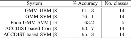
[image:2.612.312.539.304.372.2]The experiments presented here compare five automatic ac-cent recognition systems, which differ in their architectures and pre-processing requirements. These will be compared with similar systems which were developed in past studies and tested on other corpora. Four similar systems to those which were developed in [8] will be used (GMM-UBM, GMM-SVM, ACCDIST-based Correlation, ACCDIST-based SVM), as well as one from [13] (Phonological GMM-SVM). The systems in [8] were tested on theAccents of the British Isles(ABI) cor-pus [14], which comprises 14 different accents from across the breadth of the British Isle. The system in [13], however, was tested on a database of five Flemish varieties. The table below displays the results from these past studies.
Table 1:Recognition rates generated by accent recognition sys-tems in past studies.
System % Accuracy No. classes GMM-UBM [8] 61.13 14 GMM-SVM [8] 76.11 14 Phon-GMM-SVM [13] 63.2 5 ACCDIST-based-Corr [8] 93.17 14 ACCDIST-based-SVM [8] 95.18 14
It is important to acknowledge the number of accents in-volved in each of the studies. In [8], they were distinguish-ing between 14 varieties dispersed across the British Isles. The chance expectations of that study’s systems is therefore 7.1%, and we can see from the table above that each of the different architectures achieve rates which are well above this. We can of course observe a spread of results across the systems with the text-independent systems (GMM-UBM and GMM-SVM) striking recognition rates which are much lower than the text-dependent systems (the ACCDIST-based systems).
In the case of the Phonological-GMM-SVM system from [13], the chance expectation attached to the result above is 20.0%, as their study involved distinguishing between only five Flemish varieties. Given this, the result of 63.2% does not seem as impressive. However, they claim that the varieties they were distinguishing between were quite similar. Even though Flanders is known to have very distinct dialects for such a geographically-enclosed area, when speakers speak the stan-dard language, differences between the groups are less promi-nent. Performing accent recognition on these kinds of databases could be useful to forensic applications. It is perhaps of inter-est to assess how sensitive accent recognition systems can be to varieties which are more alike.
This study will bring these different types of systems to the AISEB corpus (Accent and Identity on the Scottish/English Border corpus [15]). We will compare the results brought about by these past experiments with those generated using variants of these systems on the AISEB corpus.
3. A Comparison of
Automatic Accent Recognition Systems
3.1. System 1: GMM-UBM
[image:3.612.368.486.71.237.2]A Universal Background Model (UBM) is trained using multi-speaker speech data including all the accents involved. MFCCs are extracted throughout the speakers’ speech samples (using the HTK toolkit [16]). These are composed of 12 coefficients, plus energy, and in addition, delta and acceleration coefficients are appended to the vector, totalling to 39 elements. These are extracted from 25ms windows of speech at overlapping 10ms intervals. Accent-specific multi-speaker speech data for each accent in the corpus is then introduced to the training process as enrolment data. For each set of enrolment data, MFCCs are ex-tracted and MAP adaptation [17] is applied to adapt an accent-specific model: a representative accent-accent-specific GMM. To clas-sify a test speaker, the likelihood of the test speaker’s acoustic features belonging to each of the adapted models is calculated. The highest probability determines the speaker’s accent class.
Figure 1:Flow diagram of a GMM-UBM system.
3.2. System 2: GMM-SVM
[image:3.612.114.228.258.432.2]In the same way as System 1 above, a UBM is trained using multi-accent, multi-speaker speech data. In the case of this sys-tem, the enrolment data is speaker-specific, but still independent of spoken content. Instead of adapting one single model to rep-resent one accent, a model is adapted for each of the speakers in the enrolment data. This leaves multiple GMMs representing each accent. Taking each of these speaker-specific GMMs, for each of the accent groups, the means are taken and concatenated to form a vector, which represents each speaker. These are fed into a Support Vector Machine (SVM) and effectively plotted in multi-dimensional space, while all other speakers’ GMM means of all other accent classes are also fed in to form a ‘one-against-the-rest’ configuration. An optimal ‘hyperplane’ between the accent class and ‘the rest’ is formed. On rotation, each accent class forms an SVM this way. In testing, an unknown speaker’s speech sample is used to adapt a model from the UBM and the mean vector is introduced to each SVM formed for each accent class. The accent label is determined by the clearest margin it forms with the hyperplane.
Figure 2:Flow diagram of a GMM-SVM system.
3.3. System 3: Phonological GMM-SVM
The training speakers’ speech samples, along with their ortho-graphic transcriptions, for each of the accents involved are taken and forced aligned. Using these alignments, a GMM is trained to represent each phoneme for an individual speaker. All the GMM means for each phoneme are concatenated to represent the speaker’s pronunciation system in one long supervector. In the same way as System 2, each of the training speakers’ rep-resentative vectors are fed into a SVM. To classify an unknown speaker, the speech sample and transcription are forced aligned and subsequently used to train phoneme-specific GMMs. The means of these GMMs are concatenated into a supervector and introduced to the SVM to assign an accent label.
Figure 3:Flow diagram of a Phonological GMM-SVM system.
3.4. System 4: Y-ACCDIST-Correlation
[image:3.612.364.494.441.635.2]for each English vowel phoneme. A representative matrix is formed by calculating the Euclidean distance between all vowel phoneme pair combinations, which aim to capture telling intra-speaker phonemic differences, indicative of an individual’s ac-cent. For example, the vowels infootandstrutare more similar for a typical Northern English English speaker than they are for a typical Southern English English speaker. The Euclidean dis-tance between these two vowel phonemes, then, is expected to be smaller for the Northern speaker than it is for the Southern speaker. The matrix is intended to capture these sorts of differ-ences. For each accent class in the database, each speaker’s ma-trix belonging to the group is taken and an average ACCDIST matrix is calculated to represent that accent.
Figure 4:Illustration of part of an ACCDIST matrix.
[image:4.612.341.508.257.432.2]For classification, an unknown speaker’s speech sample, along with a transcription, is converted into a representative ACCDIST matrix (in the way just described above). Pearson product-moment correlation is calculated (as per [18]) between the unknown speaker’s matrix and each of the representative accent matrices. The unknown speaker’s accent label is deter-mined by the accent class it generates the highest correlation value with, which indicates a higher degree of similarity.
Figure 5:Flow diagram of the Y-ACCDIST correlation system.
3.5. System 5: Y-ACCDIST-SVM
Speakers are processed as above (in Section 3.4) to model a rep-resentative ACCDIST matrix for each speaker. The difference between systems 4 and 5, however, lies in the classification pro-cess. For each accent class, the speaker matrices belonging to that class are fed into an SVM (in the same way as the GMM-SVM system) and the ACCDIST matrices for all other speakers of all other accents are fed in to form a ‘one-against-the-rest’ configuration. The accent classes rotate, so each becomes the ‘one’ in an SVM. An optimal hyperplane is formed for each configuration between the accent class and ‘the rest’. When classifying an unknown speech sample, it is converted into an ACCDIST matrix and subsequently incorporated into each of the SVMs produced for each accent class. The accent class la-bel is decided based on the clearest margin formed between the unknown speaker and the hyperplane in each of the SVMs.
Figure 6:Flow diagram of the Y-ACCDIST-SVM system.
4. Experiments
All five systems described above were trained and tested using the same data for comparison. The database used is described in the section below.
4.1. The AISEB Corpus
The Accent and Identity on the Scottish/English Border (AISEB) corpus [15] was used for the present study. It consists of speakers from four locations along the Scottish English bor-der: Berwick-upon-Tweed, Eyemouth, Carlisle and Gretna. For the purposes of this study, a total of 120 speakers were used: 80 speakers were used to train each system, while 40 were used for testing. The AISEB corpus provides a recorded wordlist, read-ing passage and interview for each speaker. The results in this study are generated using the reading passage recording only (sampled at a rate of 44.1kHz). This amounted to approximately 3 minutes of speech per speaker.
4.2. Results
[image:4.612.91.252.444.698.2]Table 2: Recognition rates for each accent recognition system classifying the 40 test AISEB speakers into one of four accent groups (25% correct expected at chance).
System % Correct GMM-UBM 37.5
GMM-SVM 35.0 Phon-GMM-SVM 62.5
Y-ACCDIST-Corr 82.5 Y-ACCDIST-SVM 87.5
[image:5.612.101.242.118.187.2]The text-independent systems (UBM and GMM-SVM) perform above chance level, but not by much. We can compare these results with those generated by similar systems in past studies (in Table 1). We witness a similar hierarchy of systems with regards to their relative performance. However, the spread of performance appears to be much more dramatic when applying these sorts of systems to the AISEB data. We still seem to see a drop in performance by the ACCDIST-based systems, but they appear to be much more robust to these kinds of task. Also of note are the confusion matrices for each of the systems displayed in the tables below:
Table 3:GMM-UBM system confusion matrix.
Location Ber. Car. Eye. Gre.
Ber. 6 2 0 2
Car. 3 3 2 2
Eye. 2 2 5 1
[image:5.612.92.249.345.401.2]Gre. 5 4 0 1
Table 4:GMM-SVM system confusion matrix
Location Ber. Car. Eye. Gre.
Ber. 4 3 1 2
Car. 2 5 3 0
Eye. 1 5 3 1
Gre. 3 5 1 1
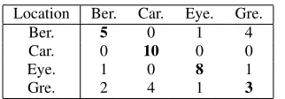
Table 5:Phon-GMM-SVM system confusion matrix
Location Ber. Car. Eye. Gre.
Ber. 5 0 1 4
Car. 0 10 0 0
Eye. 1 0 8 1
Gre. 2 4 1 3
Table 6:Y-ACCDIST-Correlation system confusion matrix
Location Ber. Car. Eye. Gre.
Ber. 9 1 0 0
Car. 2 7 0 1
Eye. 0 0 10 0
[image:5.612.95.251.446.505.2]Gre. 0 1 2 7
Table 7:Y-ACCDIST-SVM system confusion matrix
Location Ber. Car. Eye. Gre.
Ber. 10 0 0 0
Car. 2 6 0 2
Eye. 0 0 10 0
Gre. 0 0 1 9
The small amount of test data used for these experiments must be kept in mind. However, they may still be able to shed light on some considerations for further developments on au-tomatic accent recognition systems. One consideration is that some accent groups might be more likely to be successfully classified by one system over another. For example, in the ma-trices above, all Carlisle speakers are correctly classified by the Phon-GMM-SVM system, but as a group, Carlisle speakers are correctly classified on fewer occasions by the two overall more successful Y-ACCDIST systems. Other accent groups perhaps show a preference for the Y-ACCDIST-based systems. To make this observation more substantial, a greater pool of test speak-ers would be required, but these observations still open up lines of inquiry into system fusion, where different types of systems are combined with the intention of improving overall recogni-tion rate. One way in which fusion might be done is by using multi-class linear logistic regression (as per [8]’s acoustic-fused accent recognition system), but a much larger dataset would be required.
5. Feature Selection
Another aspect we can assume is affected by the data, or spe-cific accent varieties involved, is the particular segmental com-bination which would be most valuable to a given accent clas-sification task. In their accent clasclas-sification experiments on Flemish accents, [13] applied feature selection methods to a text-dependent GMM-SVM system, seeing an improvement in overall performance. Two feature selection methods they used were one-way ANOVA and SVM-RFE (Support Vector Machine Recursive Feature Elimination). Taking the highest-performing accent recognition system from the experiments above (Y-ACCDIST-SVM), the descriptions below will outline how these two methods are applied to the Y-ACCDIST matrices before the final SVM classification stage takes place.
5.1. Analysis of Variance (ANOVA)
ACCDIST matrices for the training speakers are formed using both vowels and consonants. For each accent involved, the in-dividual speaker matrices of that accent are grouped together to form an average accent matrix and passed through the one-way ANOVA. The individual elements of each of the Y-ACCDIST matrices are then ranked according to how statistically signif-icant they are, indicated by theirp-value. This suggests how much distinctive value the particular element, i.e. the specific similarity relationship between the two phonemes, brings to distinguishing between the varieties. A selection of only the top-ranked elements can then be introduced to the classification process.
5.2. SVM-RFE
[image:5.612.93.254.549.605.2] [image:5.612.94.249.652.707.2]and consonants were included, as with the ANOVA method). A SVM is trained in the usual way and, one by one, each feature of the Y-ACCDIST matrix is removed and classification perfor-mance is monitored. The feature which improved the system’s performance the most through its absence is ranked as the least valuable feature to the task. It is then removed from the rest of the process and the RFE continues to identify the least valuable matrix element for each iteration. The result is a ranked list of Y-ACCDIST matrix elements in order of distinctive potential for the given accent recognition task.
5.3. Experiments
[image:6.612.68.289.389.519.2]The effects of these methods were measured via the accent recognition performance of the Y-ACCDIST-SVM system. AC-CDIST matrices for the training speakers of each accent were formed using all the vowels and consonants in the phoneme in-ventory. The baseline classification rate in this configuration is 80.8% correct, contrasting with the Y-ACCDIST-SVM result presented above, where only vowels were used (86.7% correct). In increments of five, the topnmatrix elements, ranked by each feature selection method were the only elements which represented each speaker’s accent to form an ACCDIST matrix. These reduced ACCDIST matrices were then fed into the SVM classifier and tests were conducted as normal. These recogni-tion rates, where increasing numbers of matrix elements are used (along thex-axis), are shown in the graph below.
Figure 7: Graph to show recognition performance of Y-ACCDIST-SVM when varying the numbers of the top-ranked Y-ACCDIST matrix elements, determined by ANOVA and SVM-RFE.
The horizontal line is the baseline recognition level of this accent recognition task when all vowels and consonants are pro-cessed through the system (80.8% correct).
We can witness the two feature selection methods behav-ing slightly differently. SVM-RFE seems to more consistently achieve a recognition rate above baseline, whereas ANOVA achieves the highest recognition rate overall (89.2% correct). This is achieved by only using the top 80 ranked matrix ele-ments.
Obviously, these feature selection methods have been im-plemented with the primary intention of improving recognition rates. However, this feature may be useful to forensic ana-lysts, as well as to sociophonetic research. These methods offer an improvement to overall performance, and so it is assumed that these methods are identifying the most useful segmental
features. This might be valuable when we are dealing with unfamiliar or particularly under-researched varieties. These techniques might be able to provide a new way of screening databases of accent varieties.
6. Summary and Discussion
The first part of this paper has revealed a broad spectrum of results when five different systems (text-dependent and text-independent architectures) were tested on geographically-proximate accents. A comparison of these results with past studies confirms that we cannot assume that recognition results generated from one corpus will be reflected when the same tems are tested on another. It has been shown that some sys-tem types suffer more than others when challenged by a set of more similar accent varieties. However, it might be the case that when the systems are faced with other types of challenges (e.g. degraded and mismatched speech data, some systems may do better than others. This opens up a number of avenues for further research.
The second part of this paper focussed on ways in which we might be able to automatically identify Y-ACCDIST matrix elements (therefore phoneme pair distances) are the most useful in a given accent classification task. Experiments showed that by statistically eliminating the lower-ranking matrix elements, classification rate improves. It might be the case that other methods of feature selection may be better for this purpose. Fur-ther exploration into alternative feature selection methods might therefore give way to higher recognition rates.
While the current paper has shed light on aspects we should bear in mind when applying such systems to a corpus, and also uncovered additional strategies which can improve per-formance, the data used are still at a distance from the reali-ties faced by forensic analysts. The data used here were good-quality reading passage recordings. To put automatic recogni-tion systems to the test, further research must reflect the sorts of tasks faced by forensic speech scientists in real-life case-work. In future research, a greater focus will therefore be on how automatic accent recognition systems perform on content-mismatched speech data (spontaneous speech data), rather than using reading passage data. The comparison of systems should also include an i-vector classification system, similar to those presented in [9]. Additionally, degraded recordings of tele-phone quality will also be used for testing.
7. References
[1] Georgina Brown, “Y-ACCDIST: An automatic accent recognition system for forensic applications,” M.S. the-sis, University of York, UK, 2014.
[2] Yanli Zheng, Richard Sproat, Liang Gu, Izhak Shafran, Haolang Zhou, Yi Su, Dan Jurafsky, Rebecca Starr, and Su-Youn Yoo, “Accent detection and speech recognition for shanghai-accented mandarin,” 2005, pp. 217–220.
[3] Maryam Najafian, Andrea DeMarco, Stephen Cox, and Martin Russell, “Unsupervised model selection for recog-nition of regional accented speech,” inProceedings of In-terspeech, Singapore, 2014, pp. 2967–2971.
[5] M. Huckvale, “ACCDIST: An accent similarity metric for accent recognition and diagnosis,” inSpeaker Classifi-cation, C M¨uller, Ed., vol. 2 ofLecture Notes in Com-puter Science, pp. 258–274. Springer-Verlag, Berlin Hei-delberg, 2007.
[6] Marc Zissman, “Comparison of four approaches to auto-matic language identification of telephone speech,”IEEE Transactions on Speech and Audio Processing, vol. 4, pp. 31–44, 1996.
[7] Fadi Biadsy, Hagen Soltau, Lidia Mangu, Jiri Navratil, and Julia Hirschberg, “Discriminative phonotactics for dialect recognition using context-dependent phone clas-sifiers,” in Proceedings of Odyssey: The Speaker and Language Recognition Workshop, Brno, Czech Republic, 2010, pp. 263–270.
[8] Abualsoud Hanani, Martin Russell, and Michael Carey, “Human and computer recognition of regional accents and ethnic groups from British English speech,” Computer Speech and Language, vol. 27, pp. 59–74, 2013.
[9] Andrea DeMarco and Stephen Cox, “Iterative classifica-tion of regional british accents in i-vector space,” in Pro-ceedings of Machine Learning in Speech and Language Processing, 2012.
[10] Mohamad Hasan Bahari, “Accent recognition using i-vector, guassian mean supervector and gaussian poste-rior probabillity supervector for spontaneous telephone speech,” inProceedings of the International Conference on Acoustics, Speech and Signal Processing (ICASSP), 2013, pp. 7344–7348.
[11] Utpal Bhattacharjee and Kshirod Sarmah, “GMM-UBM based speaker verification in multilingual environments,”
International Journal of Computer Science Issues, vol. 9, pp. 373–380, 2012.
[12] V Vapnik,Statistical Learning Theory, Wiley, New York, 1998.
[13] Mark Huckvale, “ACCDIST: a metric for comparing speakers’ accents,” inProc. International Conference on Spoken Language Processing, Jeju, Korea, 2004, pp. 29– 32.
[14] Tingyao Wu, Jacques Duchateau, Jean-Pierre Martens, and Dirk Van Compernolle, “Feature subset selection for improved native accent identification,” Speech Communi-cation, vol. 2, pp. 83–98, 2010.
[15] Shona D’Arcy, Martin Russell, Sue Browning, and Mike Tomlinson, “The accents of the British Isles (ABI), corpus,” in Proceedings of Modelisations pour l’Identification des Langues, Paris, France, 2004, pp. 115– 119.
[16] Dominic Watt, Carmen Llamas, and Daniel Ezra Johnson, “Sociolinguistic variation on the Scottish-English border,” inSociolinguistics in Scotland, R. Lawson, Ed., pp. 79– 102. Palgrave Macmillan, London, 2014.
[17] S Young, G. Evermann, M. Gales, T. Hain, D. Ker-shaw, X. Liu, G. Moore, J. Odell, D. Ollason, D. Povey, V. Valtchev, and P. Woodland, The HTK Book for HTK Version 3.4, Cambridge University Engineering Depart-ment, Cambridge, 2009.
[18] Jean-Luc Gauvain and Chin-Hui Lee, “Maximum a-posteriori estimation for multivariate gaussian mixture ob-servations of Markov chains,” IEEE Transactions on Speech and Audio Processing, vol. 2, 1994.
[19] Emmanuel Ferragne and Franc¸ois Pellegrino, “Auto-matic dialect recognition: A study of British English,” in