(will be inserted by the editor)
Dynamic stochastic block models
Parameter estimation and detection of changes in community structure
Matthew Ludkin · Idris Eckley · Peter Neal
Received: date / Accepted: date
Abstract The stochastic block model (SBM) is widely used for modelling network data by assigning individu-als (nodes) to communities (blocks) with the probabil-ity of an edge existing between individuals depending upon community membership. In this paper we intro-duce an autoregressive extension of the SBM, based on continuous-time Markovian edge dynamics. The model is appropriate for networks evolving over time and al-lows for edges to turn on and off. Moreover, we allow for the movement of individuals between communities. An effective reversible jump Markov chain Monte Carlo algorithm is introduced for sampling jointly from the posterior distribution of the community parameters and the number and location of changes in community mem-bership. The algorithm is successfully applied to a net-work of mice.
Keywords Stochastic Block Model · autoregressive Dynamic Network · Reversible jump MCMC · Continuous Time Network
We gratefully acknowledge the support of the EPSRC funded EP/H023151/1 STOR-i Centre for Doctoral Training
M. Ludkin
E-mail: [email protected]
STOR-i Centre for Doctoral Training, Department of Math-ematics and Statistics, Lancaster University, Lancaster, LA1 4YF, UK
I. Eckley
STOR-i Centre for Doctoral Training, Department of Math-ematics and Statistics, Lancaster University, Lancaster, LA1 4YF, UK
P. Neal
Department of Mathematics and Statistics, Lancaster Uni-versity, Lancaster, LA1 4YF, UK
1 Introduction
Network models play a key role in capturing and un-derstanding population dynamics in a range of scenar-ios. Networks often show some form of structure rather than simple random interactions and this has led to a plethora of network models to capture such dynamics. Structures studied in the literature include: Barabsi-Albert model (Barabsi-Albert and Barab´asi 2002) (a scale-free model generated by preferential attachment), Watts-Strogatz model (Watts and Watts-Strogatz 1998) (small-world model), exponential random graph model (ERGM)(Frank and Strauss 1986) (specified frequencies of subgraphs) and the stochastic block model (SBM) (Frank and Harary 1982) (community model). This body of research cov-ers a broad range of subject areas including the social sciences, statistics, physics and computational biology. In this paper we consider the statistical detection of changes in the community structure of a dynamic network. The challenge of detecting changes in data se-quences is well-known, receiving considerable attention in the statistics literature in recent years. Much of this effort has been focused on changepoint detection within univariate data sequences, for example, see Davis et al (2006); Fearnhead and Liu (2007); Picard et al (2007); Killick et al (2012); Fryzlewicz (2014); Haynes et al (2017). More recently, the literature has turned to fo-cus on the detection of changes in more complex set-tings including multivariate time series (e.g. Matteson and James (2014); Xie and Siegmund (2013), spatial-temporal (Altieri et al 2015) and related challenges with network data (e.g. Fu et al (2009); Yang et al (2011); Xu and Hero (2014); Matias and Miele (2016)).
an-other with the interactions between individuals depend-ing upon their community. Animals changdepend-ing their mat-ing partners is a prime example of such behaviour. De-tecting changes in community structure in animal herds could help indicate the source of disease outbreaks and help with decisions such as targeted vaccination pro-grams. In Section 6, we study the changes in commu-nity structure in a network of mice first presented in Lopes et al (2016b).
The different network models described above typ-ically capture different network features. For example, the Watts-Strogatz model can create clusters whilst keeping a small distance between any two chosen nodes. This model has no simple parametric form, hence non-parametric methods are used to assess model fit (Ko-laczyk 2009). The ERGM can create clusters of nodes with specified sub-graph properties but is known to suf-fer from identifiability problems (Chatterjee and Diaco-nis 2013) since two different parameterisations can lead to the same model. Given that our primary interest is in community dynamics, we focus on a dynamic, autore-gressive extension of the SBM, introduced by Holland et al (1983). The general form of the SBM model is given by Snijders and Nowicki (1997) who discuss max-imum likelihood estimation and an Expectation Max-imisation algorithm for inferring the parameters for the SBM. The SBM aims to partition the set of nodes in a network in such a way that the proportion of edges between nodes in the same block is different to the pro-portion of edges between nodes in different blocks.
In this paper, the autoregressive stochastic block model (ARSBM) is introduced. This model is inspired by populations where the network of contacts (edges) between individuals evolve over time and depend upon the community (block) to which individuals belong; see, for example, the mice network data, Section 6 and Lopes et al (2016b). The edges are binary states 1/0 which alternate between being on (1) and off (0), spend-ing time in a given state before transitspend-ing to the other state. The observed data consist of snapshots of the network over time with snapshots close together in time typically being more similar to those further apart. The correlation in the presence/absence of edges is a key fea-ture of the data we want to explore and capfea-ture in our modelling. In addition, we seek to infer other important characteristics of the population such as the amount of movement of individuals between communities (blocks) and the interactions both within and between blocks.
There have been a number of extensions of the SBM to include temporal dynamics. Various authors have considered a continuous-time model based on an SBM where the edge processes are non-homogeneous Pois-son point processes (DuBois et al 2013; Guigour`es et al
2015; Corneli et al 2016; Xin et al 2017; Matias et al 2017). This is appropriate for event data such as send-ing emails or SMS. However, for edge processes which have a duration, such as phone calls and the status of friendships in a social network, a model which accounts for the time for which an edge lasts is required. Another direction which has attracted attention is discrete time dynamic extensions of the SBM (Fu et al 2009; Yang et al 2011; Xu and Hero 2014; Matias and Miele 2016). These papers have focused on discrete-time dynamics for both community membership and the network evo-lution over time. A key assumption of these works is that, conditional upon the community structure, the networks at each time point are independent SBMs. Re-laxing the time-independence assumption is an impor-tant contribution of this work with a view to application domains with highly correlated edges. For example, in a computer network, knowing that two machines are currently connected means they are more likely to be connected in the near future. Moreover, as we show in this article, some community structures can only be de-tected by taking account of the temporal dependencies in the network dynamics. Finally, the continuous-time model handles irregularly observed or incomplete data far more easily than its discrete-time counterparts.
simu-lated data sets and a data set involving monitoring so-cial behaviour in mice (Lopes et al 2016b), respectively. Finally, in Section 7 we make some concluding remarks concerning directions for future research in this area.
2 The autoregressive stochastic block model 2.1 Model
The autoregressive stochastic block model (ARSBM) is built on a hierarchical structure as follows. Suppose a dynamic network consists of a fixed set of nodes, V (|V|=N), partitioned into a fixed number of commu-nities,K. The community membership of theN nodes is modelled using N independent and identically dis-tributed community membership processes. Let Ci(·) denote the community membership process for nodei. It is assumed that Ci(·) is a continuous-time Markov chain (CTMC) (Norris 1997), which takes values in {1,2, . . . , K}, with Ci(t) = k meaning that individ-ual i is in community k at time t. We assume that, regardless of the current community to which it be-longs, a node spends Exp(λ) time in the community before moving to a new community chosen uniformly at random from the remaining communities. (This as-sumption can easily be relaxed.) Therefore the genera-tor matrix for the CTMC governingCi(·) has diagonal elements equal to−λand off-diagonal elements equal to λ/(K−1). Using properties of CTMCs, the number of times nodeichanges community,Mi ∼Po(λ) with the times of the changes τi = (τi1, . . . , τ
Mi
i ) being ordered and uniformly distributed on [t0, tT]. The new commu-nity level,Ci(τid), is drawn uniformly at random from
{k=6 ci(τid−1) :k= 1, . . . K}, and individualiremains in that community until τid+1. Throughout we denote the stochastic process by Ci(t) and a given realisation at timet byci(t).
In the SBM the probability that an edge exists be-tween two nodes depends only upon the communities to which the two nodes belong. In the ARSBM, we employ a similar model hierarchy with edge dynamics only depending upon the communities to which the two nodes belong. We introduce an autoregressive compo-nent which allows the state of the edge to switch “on” or “off” with Markovian dynamics. We make the ad-ditional assumption that all edges with end-nodes in different communities have similar dynamics, although this can easily be relaxed. Under this setting, there will be K+ 1 processes to govern the dynamics of edges in the network: one process for each community k (gov-erning the edges (i, j) with Ci(t) = Cj(t) = k) and one process for edges between communities (governing
the edges (i, j) whereCi(t)6=Cj(t)). This reduces the number of parameters fromO(K2) toO(K).
In order to model edge dynamics, we first define the community membership of the edge, which is a deter-ministic function of the community membership of the end-nodes. Specifically, for the edge between nodes i andj, its community membership processCij(·) is de-fined to bekif bothiandj are in communitykand 0 otherwise, as in Equation (1).
Cij(t) =
(
Ci(t) ifCi(t) =Cj(t), 0 ifCi(t)6=Cj(t),
Cij(t)∈ {0,1, . . . , K}.
(1)
Since bothCi(·) and Cj(·) are piecewise constant pro-cesses, thenCij(·) is a piecewise constant process with
Mij ≤ Mi +Mj step changes. Let Eij(·) denote the edge status process for the edge between nodesiandj. Specifically,Eij(t) = 1 if an edge exists (“on”) between nodesiandj at timetandEij(t) = 0 if no edge exists (“off”) between nodesiandj at timet. The edge pro-cess is assumed to follow a piecewise time-homogeneous CTMC. That is, whilst the Cij(t) = k, the generator matrix for the edge process is
G(k) =
−αk αk
δk−δk
.
The transition rates αk, referred to as theappearance
rates, govern the rate at which an edge appears (tran-sitions from state 0 to 1) whilst in communityk. Simi-larly, the transition ratesδk are referred to asdeletion
ratesand govern the reverse transition from state 1 to 0. Throughout, we denote the stochastic process byEij(t) and a given realisation at timetbyeij(t).
Letπk=αk/(αk+δk), the stationary probability of an edge being on in communityk. This allows for a di-rect comparison with the static SBM. Furthermore, let ρk=αk+δkbe the combined rate of change for the edge process withαk =πkρk andδk = (1−πk)ρk. It is help-ful to use the parameterisation π = (π0, π1, . . . , πK) andρ= (ρ0, ρ1, . . . , ρK) for modelling the ARSBM.
2.2 Posterior distribution
We are now in position to construct the likelihood for the data and the posterior distribution of the parame-ters and community membership of the nodes.
between nodesiandjat thesthobservation. Similarly, cs
i =ci(ts) is the community membership of nodei at observation time s; however, this is a latent variable. We also let ∆s =ts−ts−1 be the amount of time be-tween observations s−1 and s. Let e(t) = {es
ij|1 ≤
i < j ≤N, s = 0,1, . . . , T} denote the set of all net-work snapshot data. Let ci(t) = {csi|s = 0,1, . . . , T}, the community membership of node i at every obser-vation time, with c(t) = {ci(t)|i = 1,2, . . . , N}, the set of all community memberships. We are interested in the joint posterior distribution, which can be decom-posed into the product of the observation likelihood, the distribution of the evolution of community assign-ments and a prior distribution on the parameters as in Equation (2).
π(θ,c(t)|e(t))∝π(e(t),c(t)|θ)π(θ)
=π(e(t)|c(t),θ)π(c(t)|θ,c(t0))π(θ,c(t0)), (2) where θ = (λ,π,ρ) and c(t0) = (c0
1, c02, . . . , c0N). Note the dependence on the initial community structure.
We now provide equations for each term in Equa-tion (2). Firstly, in EquaEqua-tion (3), the likelihood of the observed edge sequence, given the latent community memberships and model parameters, is computed.
π(e(t)|c(t),θ) =Y s,i j6=i
π(esij|esij−1, cis−1, csi, csj−1, csj) (3)
The computation of each factor in Equation (3) is non-trivial since it requires integrating over all possible com-munity membership processes for all nodes between the times ts−1 and ts. Since each community membership process is piecewise constant, it is sufficient to know the times of the changepoints in node i’s community membership, τi = (τi1, . . . , τ
Mi
i ), and the community membership of the nodes at the changepoints, ci(τi) with c(τ) = (c1(τ1), . . . ,cN(τN)). Note that cij(τij) is a deterministic function of ci(τi) andcj(τj), where
τij = (τij1, . . . , τ Mij
ij ) is the set of combined change-points in nodes iandj community memberships.
Therefore, given that the edge dynamics are gov-erned by a CTMC with piecewise constant dynamics then, ifcij(t) =kfor all timet∈[ts−1, ts), then
P es= 1|es−1, c(t)
=πk+ (es−1−πk)e−ρk∆s, (4)
where we drop the subscriptij for brevity.
The calculation of the probability of an edge being in state 1 becomes more involved if there is a change in community membership of the edge during an interval [ts−1, ts). It is straightforward, in principle at least, to compute P es
ij= 1|e s−1
ij , cij(t) by summing over the possible states of the edgeijat each of the changepoints
in the interval [ts−1, ts). Specifically, ifτ ∈[ts−1, ts] is a changepoint withcij(t) =kfort∈[τ, ts), then
P es= 1|es−1, c(t)
= 1
X
l=0
P(es= 1|e(τ) =l) P e(τ) =l|es−1
= 1
X
l=0
{πk+(l−πk)e−ρk(ts−τ)}P e(τ) =l|es−1, (5)
where again, we drop the subscriptij for brevity. Whilst it is possible to computeπ(e(t)|c(t),c(τ),θ) from (5), it is far simpler to augment the data with e(τ) = {eij(τijd); 1 ≤i, j ≤ N, d = 1,2, . . . , Mij}. Let
σi=t∪τi, the ordered times at which the edges are ob-served or nodeichanges community membership. Simi-larly, letσij=σi∪σjdenote the ordered times at which edge (i, j) is observed or changes community member-ship and contains Tij =T +Mij elements. Thus, the likelihood of the observed and augmented edges, given the community structure,π(e(σ)|c(σ),τ,θ) becomes
Y
i6=j Tij−1
Y
d=0
P eij(σijd+1)|eij(σdij), cij(σijd)
(6)
where, by letting∆d+1 = (σd+1−σd), the factors can be written as:
(1−πc(σd))−(e(σd)−πc(σd))e−
ρc(σd)∆d+11− e(σd+1)
×πc(σd)+ (e(σd)−πc(σd))e−
ρc(σd)δd+1 e(σd+1)
The computation of π(c(σ),τ|θ,c(t0)) is straight-forward. Firstly,σi is deterministic givenτi, so
π(c(σ),τ|θ,c(t0)) =
N
Y
i=1
π(ci(τi)|τi,c(t0))π(τi|λ)
= N
Y
i=1
π(ci(τi)|τi,c(t0))π(τi|Mi)π(Mi|λ)
= N
Y
i=1
1 k−1
Mi
× Mi! (tT −t0)Mi
×{λ(tT −t0)}
Mi
Mi!
exp(−λ(tT−t0))
=
1
k−1
M
λMexp(−λN(tT −t0)), (7)
where M = PN
which take place and the probability that there areMi changes in nodei’s community membership.
Combining (6) and (7), we have an expression for π(e(σ),c(σ)|θ,c(t0)), and therefore, an explicit expres-sion for the right hand side of
π(c(σ),e(τ),τ,θ|e(t))∝π(e(σ)|c(σ),τ,θ)
×π(c(σ),τ|c(t0),θ)×π(c(t0),θ). (8)
2.3 Identifiability
An important point to consider before introducing the RJMCMC sampler is the identifiability of the model. As is well known for SBMs, the parameters can only be ob-tained up to a label switching of the group nodes (Ma-tias and Miele 2016). Lettingρk ↓0 for k= 0,1, . . . , K whilst keepingπfixed results inλbeing unidentifiable. This is because the graph does not change through time and hence E(t) = E(s) for all 0 ≤ s < t. Therefore the graph dynamics are invariant to how fast (or slow) the nodes switch between blocks since after the initial configuration, the block to which a node belongs be-comes irrelevant. More generally, we observe that the dependence parameterρk enters the likelihood through exp(−ρk∆s)), see Equation (4), and robust estimation of ρk is obtained when exp(−ρk∆s)) is not close to 0 (independence) or 1 (full dependence).
The graph parameters become unidentifiable asλ→ ∞, that is the nodes are constantly switching between blocks. In this case, for eachk, l= 1,2, . . . , K, the nodes i andj will spend a proportion 1/K2 time in blocksk and l, respectively during any period of time. Conse-quently, regardless of the value of K, as λ → ∞, the dynamic SBM resembles an SBM with a single block model, a dynamic Erd¨os-R´enyi random graph, with sta-tionary probability of an edgeπ∗and rate of changeρ∗, where
ρ∗= 1 K2
K
X
k=1 ρk+
K−1
K ρ0, (9)
and
π∗= 1 ρ∗
(
1 K2
K
X
k=1 ρkπk+
K−1 K ρ0π0
)
. (10)
Lettingλ→ ∞removes any dependence in block mem-bership of a node from one time point to the next. This is linked to the observation in Matias and Miele (2016) for the discrete time SBM models of Xu and Hero (2014) and Matias and Miele (2016) that inde-pendence in block membership from one time point to the next leads to non-identifiability of the parameters.
If λ = 0 and (ρk, πk) = (ρI, πI) (k = 1,2, . . . , K) (a dynamic affiliation model), then, following the ap-proach of Frank and Harary (1982) and Allman et al (2011), it is straightforward to show thatE[E12(0)] and E[E12(0)E13(0)E23(0)] give (πI, π0), as in the case of the static SBM. Moreover, consideringE[E12(0)E12(t)] andE[E12(0)E13(0)E23(0)E12(t)E13(t)E23(t)] for some t >0 is then sufficient to identify (ρI, ρ0). By consider-ing edge moments involvconsider-ing 4 nodes, we can show that this extends to small positive λ > 0 by ignoring o(λ) terms. A further discussion of parameter identifiability is beyond the scope of this paper but note that we ob-serve parameter estimation is robust to starting values in the simulations and application data set up to per-mutation of block labels, for moderate, positiveρk and small, positiveλ.
3 Reversible jump MCMC 3.1 Sampling scheme
In this section a RJMCMC (reversible jump MCMC) algorithm is described for obtaining samples from the joint posterior distribution of θ = (λ,π,ρ) and c(t) givene(t) using (8) and data augmentation of the val-ues (τ,c(τ),e(τ)). The updating of the parametersλ,π andρgiven (τ,c(τ),e(τ)) is straightforward using (6) and (7). Updating τi and the associated augmented data is more involved as Mi, the number of elements in τi, is unknown. This naturally leads to a reversible jump sampler (Green 1995) to explore parameter spaces of differing dimensions.
An overview of the sampling scheme is given in Al-gorithm 1. For each step of the sampler, each of the pa-rametersλ,π,ρ andτ (andM = (M1, M2, . . . , MN)) are updated in turn.
By assigning a Gamma(λ01, λ02) prior to λ, it fol-lows from (7) that, λ|π,ρ,τ,c(σ),e(σ) is distributed as Gamma (λ01+M, λ02+N(tT −t0)).
Forπandρthere is no closed form conditional dis-tribution and for this reason, a random walk is pro-posed. Since πk is bounded on [0,1], a random walk is proposed on a logit scale, logit(πk∗)∼N(logit(πk), σ2π). As forρk, a random walk on the log scale is proposed, sinceρk > 0, with log(ρ∗k)∼ N(log(ρk), σ2ρ). The pri-ors for πk and ρk are Beta and Gamma distributions respectively. By performing random walk updates on transformed scales, we need to take account of the pro-posal densities with
q(πk∗|πk) =
φ(logit(π∗k)|logit(πk), σ2π)
Algorithm 1RJMCMC Sampler
Inputs: parameters for Gamma prior forλ, prior distribu-tions forπandρ, nRuns and burn-in.
Drawλ, π, ρfrom their respective priors. Set M = 0 and
τ=∅.
forh=1,. . .,nRunsdo
Drawλ(h+1)from its conditional distribution.
fork in 1,. . . , Cdo
Propose π(h+1)k by taking a random walk on the
logit scale fromπk(h).
Proposeρ(h+1)k by taking a random walk on the log
scale fromρ(h)k .
if There are no changes in the current sampler state then
Propose inserting a change
elseDraw X uniformly at random from{1,2}
if X=1 then
Propose inserting a new change to the current state, with augmented edge states as required.
elseX=2
Propose deleting a change from the current state, removing and adding affected augmented edge states as required.
Given thatM > 0, propose moving each changepoint into an adjacent observation interval and using a Gaussian random walk proposal.
Resample the augmented edges. Discard samples 1, . . . ,burn-in.
and
q(ρ∗k|ρk) =
φ(log(ρ∗k)|log(ρk), σρ2)
ρk
, (12)
where φ(y;µ, σ2) denotes the probability density func-tion of aN(µ, σ2) evaluated aty.
In this work, an adaptive scheme is used to adjust the variance of the proposal distributions to improve the efficiency of the sampler. The proposal variancesσ2 π andσ2
ρ are set using an adaptive procedure as in Xiang and Neal (2014). By Roberts et al (1997), an acceptance rate of approximately 25% is optimal for random walk Metropolis sampling. To achieve this rate, a proposal varianceσ2is adjusted at each step during the burn-in period by
σ2h+1=
σh21−√ h
if move rejected, σh21 + √3
h
if move accepted,
where the step sizeis chosen as input.
3.2 Updating (τ,c(τ),e(τ))
The trans-dimensional sampler for updatingτ, and con-sequently, (c(τ),e(τ)) is now described. These consti-tute birth-death moves: inserting a changepoint (insert
a change of community membership in a node) and removing a changepoint (removes one of the changes from the current state of the sampler). In each itera-tion of the algorithm only one move is attempted. In the case that the current sampler state contains no change-points, then an insert move is attempted. Otherwise, the insert move is chosen with probability 0.5. In ad-dition, we propose moving the time of existing change-points to obtain a posterior distribution of changepoint locations.
We begin by describing the process for proposing to insert a changepoint. Firstly a nodeiis chosen uni-formly at random from 1, . . . , N and a time τ∗ is cho-sen uniformly at random from the interval [t0, tT]. This amounts to adding a step change at time τ∗ in Ci(·). Letk denote the community membership of node i at time τ∗ prior to the proposed addition of a change-point at time τ∗. Since the initial community mem-berships are unknown, the sampler allows for adjust-ingCi(·) either prior to, or after, time τ∗. A proposal “forwards” in time proposes a new communityk∗ and sets Ci(τ∗) = k∗. Conversely, a proposal “backwards” in time proposes a new communityk∗ for the interval
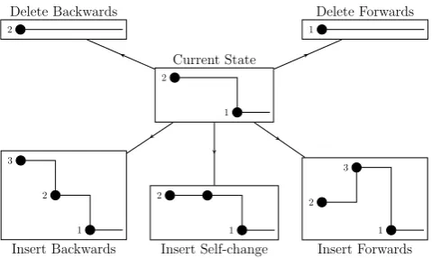
preceding τ∗. If this previous interval starts at timeσ∗, then the sampler sets Ci(σ∗) = k∗, where σ∗ = t0 if there are no previous changes in node i’s community membership with Ci(τ∗) = k. See Figure 1 for an ex-ample of possible insert moves.
2
1
Current State
2
Delete Backwards
1
Delete Forwards
3
2
1
Insert Backwards
2
1
Insert Self-change
2 3
1
Insert Forwards
Fig. 1 Possible moves to insert or delete a changepoint for a node which currently has one change. After choosing to insert or delete, a model is proposed proportional to the likelihood.
[image:6.595.297.537.464.607.2]such a change is irrelevant since inserting a self change is symmetric in time.
There are therefore 2K−1 ways to propose insert-ing a change in community membership at timeτ∗ for node i. Rather than drawing a change in community membership uniformly at random from the possibili-ties we consider the relative likelihood of the 2K − 1 changes in community membership and propose a change accordingly. In order to do this, we consider the set of edges affected by each of the proposed com-munity changes. In all cases the unobserved states of edges affected by the change are a subset ofEi(τ∗) = (Ei1(τ∗), Ei2(τ∗), . . . , EiN(τ∗)). For an edge (i, j) af-fected by the change in community membership, we augment the state space witheij(τ∗) and seteij(τ∗) = 1 with probability,
P(eij(τ∗) = 1|eij(σ∗∧t∗), cij(σ∗) =κ, πκ, ρκ), (13)
where t∗ denotes the last observation prior to τ∗. Let Ak1,k2 denote the set of additional edges proposed with
the move toci(σ∗) =k1andci(τ∗) =k2, where at least one of k1 or k2 is equal to k. Let A∗ = ∪k1,k2A
k1,k2
and note that edge (i, j) can be included in more than one Ak1,k2 with different values fore
ij(τ∗). We choose to move to community memberships ci(σ∗) = k1 and ci(τ∗) =k2 for nodeiwith probability
P Ak1,k2|θ, τ∗
P
l1,l2P(A
l1,l2|θ, τ∗). (14)
Therefore the proposal distribution for the proposed changepoint in node i’s community membership and A∗ is
P(M+ 1|M) N(tT −t0)
·P(A∗|θ, τ∗)· P A
k1,k2|θ, τ∗
P
l1,l2P(A
l1,l2|θ, τ∗). (15)
The reverse move is the deletion of a changepoint for which we require M > 0. Firstly, we select a change-point τ∗ to delete uniformly at random. Suppose that the changepoint occurs in node i’s community mem-bership. Suppose thatσ∗ denotes the previous change-point in node i prior to τ∗ and that ci(σ∗) = k1 and ci(τ∗) = k2, then there are two choices (unless k1 = k2,τ∗ represents a self-change), either set ci(σ∗) =k1 (change the future community membership from time τ∗) orci(σ∗) =k2(change the community membership prior to time τ∗). For both of these proposed changes it is possible that the set of augmented edges required changes atσ∗when settingci(σ∗) =k2and the change-point in nodei, should one exist, afterτ∗. LetBk1 and
Bk2 denote the additional augmented edges required
when settingci(σ∗) =k1andci(σ∗) =k2, respectively. For generating edges inBkl (l= 1,2), we take the same
approach as when inserting a changepoint simulating forward the state of an edge by modifying (13) to pro-pose the edge state at the required time. Then we set ci(σ∗) =kl (l= 1,2) with additional augmented edges
Bkl with probability P Bkl|θ
P(Bk1|θ) + P(Bk2|θ). (16)
Therefore, the proposal distribution for the proposed deletion of changepointτ∗with associated changes and B∗=Bk1∪ Bk2 is
P(M −1|M) M ·P(B
∗|θ)· P B kl|θ
P(Bk1|θ) + P(Bk2|θ). (17)
The generating of A∗ and B∗ in the above proce-dures are simply to assist with choosing community membership in an informed way and play no role in the posterior distribution (parameters and augmented states) once a set of augmented edges have been cho-sen. Therefore, we would ideally want to integrate out A∗ and B∗. This can effectively be done by working on an expanded state space incorporating all the pos-sible community membership states of the nodes and all possible edge states. In this way we can show that the probability of accepting a proposed move to insert a changepoint in communityiat timet∗is
π(e(σ0),c(τ0),τ0,θ|e(t)) π(e(σ),c(τ),τ,θ|e(t)) ×P(M|M + 1)N(tT−t0)
P(M + 1|M)(M + 1) ×
P(B∗|θ) P(A∗|θ, τ∗)
× P B
kl|θ P
l1,l2P A
l1,l2|θ, τ∗
P(Ak1,k2|θ, τ∗) P(Bk1|θ) + P(Bk2|θ)
(18)
where σ0 = σ∪τ∗ and τ0 = τ∪τ∗. The acceptance probability for deleting a changepoint is the reciprocal of (18).
The two procedures for moving a changepoint are straightforward. Firstly, each changepoint is moved at random either to the next observation interval or the previous observation interval. Secondly, the time of a changepoint is perturbed using a random walk move with a Gaussian proposal. The first such move allows for large changes in the location of a changepoint while the second allows for small, local moves refining the position of the changepoint. Suppose that the changepoint to be adjusted is τ which lies in the interval [tn, tn+1]. We propose a new time τ∗ to lie in one of the intervals immediately before or after [tn, tn+1]. We propose that
τ∗ is positioned in the proposed interval proportional to the location ofτ in the current interval such that:
τ∗=
(
tn−1+ (tn−tn−1)tτ−tn
n+1−tn w.p 0.5
The second move allows for refinement of such times by making a small change in location ofτusing a stan-dard Metropolis-like move. Specifically a value τ∗ is proposed viaτ∗=τ+N(0, στ) forστ small.
Finally, each augmented edge states A ∈ A∗ is re-sampled proportional to the relative likelihood using Equation (3) in the proposal distribution,
P(A= 1) = π(A= 1,e(σ)|θ)
π(A= 0,e(σ)|θ) +π(A= 1,e(σ)|θ). In the case that a changepointτ is close to an observa-tion time t, the augmented edges at τ will most likely be resampled in the same state as at the observation timet.
4 Initialisation of sampler state
In this section some observations are made about the initial community membership vector c(t0), which is key to the success of the sampler. Recall that the data e(t) concerns the state of edges in the network, which are assumed to be Markov chain distributed with pa-rameters determined by the latent community member-ship of the end nodes. These community membermember-ships are themselves Markov chain distributed conditional on the initial community assignment,c(t0). This makes the initial community membership very influential on the entire model. As such, assigning nodes to the incorrect community can lead to poor estimates for parameters πandρ, and slow convergence of the RJMCMC to the posterior distribution.
There are a number of possible ways to initialise c(t0), the initial community membership. The simplest approach is to model the initial state using a static SBM to identify the initial block assignments. Given that a single snapshot of the ARSBM is informative about π but contains no information concerning ρ, this works well if theπks (k= 1,2, . . . , K) are significantly differ-ent fromπ0. However, this approach fails ifρis the pri-mary determinant of block membership. Therefore, we propose and use throughout a robust approach based on clustering nodes using a distance metric. An alter-native clustering using a Poisson SBM on the distances was also considered. In this case, the network snapshots were projected onto a matrixMdwithMd
ij=d(i, j) for each of the distances introduced in this section. Next, an SBM with Poisson emission distribution was fitted to eachMdto yield an initial assignment of nodes to com-munities labelled cd. Finally, the assignment with the highest likelihood (under the Poisson SBM) was chosen for the initialisation. The results for using a Poisson SBM are similar to the proposed clustering method; however, the clustering procedure is faster to compute.
The distance between two nodes is the weighted av-erage of two measures. Firstly,d1(i, j) is the fraction of time thateij(·) is observed in the “on” state in the set of snapshots. Secondly,d2(i, j) is the number of times that eij(·) changes state in the set of snapshots. In essence,
d1 is a measure for π and d2 is a measure for ρ. The metric d is then a weighted average of these two dis-tances as given in (19).
d(i, j) =γd1(i, j) + (1−γ)d2(i, j) (19)
For networks where the community structure is more apparent in the ratio of edges within a community com-pared to the ratio of edges between communities, then setting γ = 1 in (19) gives a distance measure based only on this ratio. However, for networks where the community structure is embedded in the rate of tran-sition of edge states, thenγ= 0 is a more appropriate choice. This distance will work well in networks with disassortative community structures, since nodes which are less likely to be connected are close under this mea-sure. Since no assumptions are made on the assortivity of a network, the distance used should not be fixed to one type of assortivity. A further three distances are used to measure the similarity of two nodes. All four distances are given in (20).
d11(i, j) =γ11d1(i, j) + (1−γ11)d2(i, j) d10(i, j) =γ10d1(i, j) + (1−γ10)(1−d2(i, j)) d01(i, j) =γ01(1−d1(i, j)) + (1−γ01)d2(i, j) d00(i, j) =γ00(1−d1(i, j)) + (1−γ00)(1−d2(i, j))
(20)
in both the fraction of edges and the number of times edges change state. Such networks have more edges be-tween nodes in the same community compared to edges between communities which are fewer in number, how-ever the edges between communities are more persistent than edges within communities.
Using these distances, thek-means algorithm (Lloyd 1982) can be used to cluster the nodes. A good cluster-ing should separate nodes which are in different com-munities. Based on this idea, the k-means algorithm aims to put nodes which are far apart underdinto dif-ferent communities. As a result, a measure for a good clustering is the ratio R of squared distances between nodes in different communities to the total squared dis-tance between all nodes. The higher this ratio, the more separated the clusters are.
To set the initial community assignmentsc(t0), the network is measured using each of the distances in (20). Eachγparameter is set by maximisingRfor eachdby clustering the nodes usingk-means. This gives four clus-tering which are respectively optimal under each dis-tance. The clustering used to initialisec(t0) is then cho-sen as the clustering which maximises R among these four clusterings. This procedure is very quick compared to the RJMCMC sampling scheme.
5 Simulation study
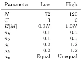
In order to assess the performance of the RJMCMC sampler, we conducted a simulation study over a range of parameter combinations. There are eight parame-ters which we varied and for each parameter we con-sidered two settings (Low, High) giving 28 = 256 pa-rameter combinations. The papa-rameter combinations are the number of nodesN, the number of communities,C, the size of each communitync, the expected number of changes E[M] (the rate of nodes moving λ) and the community parameters π and ρ. For the community parameters, we set all the within-community parame-ters to be the same, that is, for all i, j = 1,2, . . . , C, πi=πj andρi=ρj. The parameter values are given in Table 1. For equal community sizes, N/C nodes were placed in each community. The sizes of communities for other simulations are given in Table 2. We ran simula-tion for all parameter combinasimula-tions with the excepsimula-tion ofπk=π0 andρk=ρ0, where the resulting network is indistinguishable from a dynamic Erd¨os-R´enyi random graph (a stochastic block model with only one commu-nity). This yielded 192 simulated data sets, each con-sisting of 30 snapshots of the network equally spaced in time.
[image:9.595.349.484.108.209.2]The RJMCMC described in Section 3 was applied to each simulated data set forH = 20,000 steps. The prior
Table 1 Parameter settings for simulation study.
Parameter Low High
N 72 120
C 3 6
E[M] 0.3N 1.0N
πk 0.1 0.5
π0 0.1 0.5
ρ0 0.2 1.2
ρk 0.2 1.2
[image:9.595.331.500.237.279.2]nc Equal Unequal
Table 2 Number of nodes per community fornc=unequal.
N C= 3 C= 6
72 12, 24, 36 7, 9, 11, 13, 15, 17 120 20, 40, 60 10, 14, 18, 22, 26, 30
distributions for λ, π and ρ were set as Gamma(1,1), Beta(1,1) and Gamma(2,1) respectively. The algorithm was initialised with no changepoints (M = 0) and the first 1000 steps were removed as burn-in. Trace-plots of the parameters showed that the burn-in was sufficient and test runs of 50,000 steps on a subset of the data sets gave similar parameter estimates, indicating that 20,000 steps is sufficient.
In order to assess the performance of the RJMCMC algorithm the modal values, a 95% credible interval and mean absolute percentage error against the true value (MAPE, see (21)) are computed for each of the param-etersπ,ρ,λand τ. The MAPE of an estimateE from true valueT is given by:
MAPE(E, T) = n
X
i=1
|Ei−Ti|
|Ti|
(21)
Additionally, to assess the estimation of commu-nity assignments c(t), the v-measure (Rosenberg and Hirschberg 2007) was computed. V-measure is a score between 0 and 1 given to a clustering of a data set where true class labels are available Rosenberg and Hirschberg (2007). It is an information theoretic measure based on the harmonic mean of two different scores: homogene-ity and completeness. A clustering is considered homo-geneous if it assigns only those data points that are members of a single class to a single cluster, whereas a clustering is considered complete if it assigns all of those data points that are members of a single class to a single cluster. Thev-measure lies in the interval [0,1] with a v-measure of 1 denoting perfect reconstruction of the classes. Alternative metrics such as the Adjusted Rand Index (ARI) can also be used for assessing com-munity assignment.
Thev-measureVihtwas computed for each data set
step h = 1001, . . . ,20,000 of the sampler. The mean v-measure vi = Ph
P
tViht/(HT) was computed for each data set by averaging over time and sampler step. Across all sampler runs, vi has mean 0.9131 and me-dian 0.9294 with inter-quartile range [0.8856,0.9548]. Similar results were found using the ARI which had mean 0.9079, median 0.9404 and inter-quartile range [0.8644,0.9945]. The lowest v-measure was 0.6476, ob-tained for a data set with π0 =πk = 0.1 andρ0 = 0.2 and ρk = 1.2. This is a difficult data set for the sam-pler since the probability of seeing a given edge at any time is 0.1 and all the information on the community structure is encoded in the parameter ρ.
Althoughλwas estimated well in every simulation (the true value was in the HPD interval), the number of changepoints was sometimes underestimated. This generally occurred because changes close to the start or end of the observation period or that occur close to another change are difficult to detect, a well-known feature of changepoint problems. In such cases the sam-pler is performing model selection by selecting a more parsimonious model than the one simulated from. For example, in the simulation with combinedv-measure of 0.6476, the change in community memberships of nodes 26 and 63 are missed at times 1.26 and 2.03, respec-tively, and instead the sampler assigns the community they move to as their initial community. Such an early change is thus difficult to detect but may not be impor-tant since the imporimpor-tant structure (i.e.the community membership after time 2) is still captured. A similar boundary effect is present for changes late in the obser-vation period.
Finally, we investigated in more detail how the algo-rithm scales with the amount of data (N = 50,100,150; T = 20,40,60) and number of blocks (K= 2,4,6). The RJMCMC sampler run-time per iteration scales linearly with the number of snapshots and quadratically in the number of nodes which is to be expected as doubling the number of nodes quadruples the number of potential edges to evaluate. The number of blocks in the model appears to have a negligible effect on the run-time of the algorithm. For a fixed number of iterations the effective sample sizes of the MCMC output decreases slightly as N andT increase. Therefore, the main additional com-putational cost from analysing larger data sets is the larger likelihood calculations required.
6 Application: Communities of mice
In this section we apply the RJMCMC sampling scheme to a data set of mice contacts presented in Lopes et al (2016b). We aim to show how the algorithm can iden-tify changes in community structure of this dynamic
network. In this study, 90% of a population of 257 mice were observed for a period of 54 days (Lopes et al 2016a). Each nest box was fitted with a sensor which recorded when two mice were cohabiting. The data were presented as aggregates of time spent in close proximity, mainly collected every other day but with some obser-vations collected every third day. We use the data by setting the edge Yij(ts) to 1 if mice i and j had any contact on observation day ts. Since the mice sleep in nests and are social animals, it is hypothesised that the contact network will show community structure. In Lopes et al (2016b) the authors stage an intervention in some of the subjects by treating them with either lipopolyaccharide (LPS) or a placebo saline injection. It is hypothesised that treatment with LPS makes sub-jects more introverted and thus less likely to contact other subjects. The authors found that the treatment, when compared to placebo injections, reduced the de-gree to which mice interacted with others. We ask if the mice change their community structure, hypothesising that the treated mice may change community member-ship.
A preliminary analysis (Lopes et al 2016b) shows that the network is split into some disconnected com-ponents. We take a subset of 107 mice to form a sub-network. This sub-network contains some almost dis-connected components with some connections between components. This sub-network contained 12 mice who received the active treatment and 17 mice treated with a placebo. The remaining mice received no treatment.
2 4 6 8 10
0.0
0.2
0.4
0.6
0.8
1.0
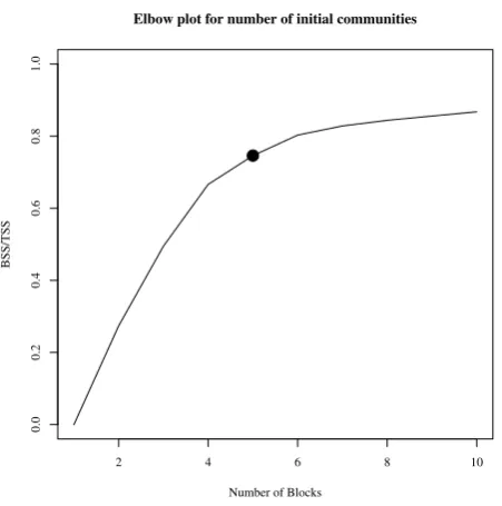
Elbow plot for number of initial communities
Number of Blocks
BSS/TSS
Fig. 2 Elbow plot for determining the number of communi-ties with which to initialise the sampler.
We ran the RJMCMC sampler for 50,000 iterations discarding the first 10,000 as burn-in. This allows the number of changes to become stable, since the sam-pler starts with zero changepoints. The estimates for the community parameters are given in Table 3 with around 50 changes in community membership. Trace-plots are available in the supplementary material. No-tice that π0 is low, showing that the communities are mainly disjointed. Contacts in communities 1, 2 and 5 are more likely than contacts in communities 3 and 4 with similar behaviour within these two groups. Note also that ρis in the range (0.4, 0.6) for all communi-ties giving a similar degree of autoregressive behaviour in the contact process for all mice. The higher value ofρ0 corresponds to a more rapid turnover of contacts between mice in different communities, as one would expect.
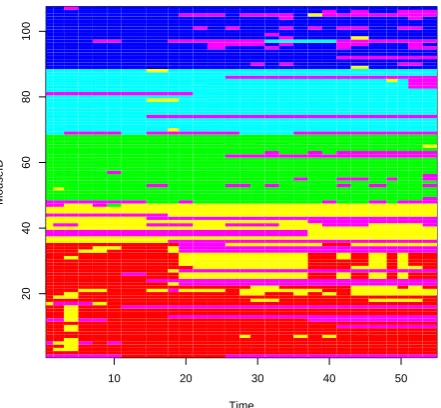
Figure 3 shows thea posteriori most probable com-munity membership through time for each mouse. The communities are coded by hatching, with the shading typezused at point (x, y) representing the highest pos-terior probability at time x of mouse y belonging to communityz. The mice detected to have changed com-munity were mainly mice which were absent from the nests over a short period. Such mice were detected to join the community labelled 6 in Figure 3. However, a few mice are more active. For example, the mouse with ID 97 leaves the nest from group 5 for some time then returns to group 4 and then leaves the nest again. For each of the 107 mice, we present plots of the
poste-rior probabilities of a mouse belonging to each of the 6 communities over time in the supplementary material. For comparison, the dynamic SBM (dynSBM) of Matias and Miele (2016) was fit to the same data. In this model, the nodes act independently and move be-tween blocks via a discrete-time Markov chain. This gives similar dynamics for the nodes as for the ARSBM. The key difference is in the modelling of the edges. Un-der dynSBM, given the block memberships of the nodes, the edges are treated as independent Bernoulli random variables. Applying the dynSBM to the mice data set yields similar memberships to those found using AR-SBM, as seen by comparing Figures 3 and 4. The mean parameter estimates for the dynSBM are given in Ta-ble 4 with some differences observed in the estimates of βk and πk, the probability of an edge existing be-tween two nodes in communitykin dynSBM and AR-SBM, respectively. This is particularly the case for com-munities 1 and 2, reflecting the significant changes in community membership seen in the dynSBM between these two communities. The dynSBM method estimates 283 changes, more than five times the mean number of changes estimated using the ARSBM, with the latter maintaining a more consistent and coherent community structure.
[image:11.595.44.270.95.323.2]Finally, we see no evidence that treating mice with LPS affects community structure of the network, (ex-cept by leaving the network). Even though mice are found to interact less by Lopes et al (2016b), those in-teractions are likely to be with the same group of mice.
Table 3 Parameter estimates for the mice community data set.
variable 5% mean 95% s.d.
M 49 52.57 56 2.0843
λ 0.0010 0.0019 0.0030 0.0006
π0 0.0003 0.0004 0.0005 0.0001 π1 0.6799 0.6994 0.7182 0.0118 π2 0.6111 0.6660 0.7189 0.0328 π3 0.4152 0.4349 0.4547 0.0121 π4 0.4331 0.4473 0.4609 0.0084 π5 0.6616 0.6821 0.7007 0.0119 ρ0 1.1489 1.3164 1.5059 0.1092 ρ1 0.4740 0.5138 0.5556 0.0248 ρ2 0.3420 0.4104 0.4893 0.0453 ρ3 0.5256 0.5650 0.6054 0.0244 ρ4 0.3915 0.4077 0.4246 0.0102 ρ5 0.6265 0.6851 0.7429 0.0357
7 Concluding remarks
[image:11.595.319.510.511.660.2]10 20 30 40 50
20
40
60
80
100
Time
MouseID
Fig. 3 ARSBM: Maximum a posteriori community membership of each mouse through time. Community labels are: 1 -red, 2 - yellow, 3 - green, 4 - sky blue, 5 - dark blue, 6 - purple. These labels match the parameter labels in Table 3.
Table 4 Parameter estimates for the mice community data set from the dynSBM (β) and ARSBM (π, ρ).
k βk πk ρk
0 0.0948 0.0004 1.3164 1 0.3645 0.6994 0.5138 2 0.7301 0.6660 0.4104 3 0.6415 0.4349 0.5650 4 0.5610 0.4473 0.4077 5 0.7602 0.6821 0.6851
and an effective RJMCMC algorithm to sample jointly from the posterior distribution of the parameters and the number and location of individuals’ changes in com-munity membership. The Markovian nature of the AR-SBM makes it flexible and allows the model and RJM-CMC algorithm to be trivially applied to irregularly ob-served data or data with gaps in the collection process, both of which are challenging problems for discrete-time models. The effectiveness of the RJMCMC algorithm is demonstrated through the simulation study with excel-lent detection of the changepoints in community mem-bership. There are a number of exciting avenues for future research opened up by autoregressive stochas-tic block models. Firstly, whilst the initialisation pro-cedure for community allocation worked well in the ex-amples in this paper, alternative clustering algorithms could be considered, especially by estimating the com-munity structure throughout the observation interval. This would enable the insertion of changepoints into the model at the start of the RJMCMC algorithm to
10 20 30 40 50
20
40
60
80
100
Time
MouseID
Fig. 4 dynSBM: Trace for community membership of each node. Community labels are: 1 - red, 2 - yellow, 3 - green, 4 - sky blue, 5 - dark blue, 6 - purple. These labels match the parameter labels in Table 4.
reduce the potentially lengthy burn-in period. Secondly, it would be useful to allow the number of communities to be an unknown parameter which possibly varies over time. This would avoid the use ofad hocmethods such as an elbow plot to choose the number of communities and, more interestingly, allow the number of communi-ties to vary through time, with the possibility of large global changes when communities split or merge. Fur-ther possible extensions include covariate information on edges or nodes and weighted edges. Both of these present challenges in efficient evaluation of the likeli-hood as in this paper we have been able to exploit the binary state of edges classified solely by the community membership of the nodes.
References
Albert R, Barab´asi AL (2002) Statistical mechanics of com-plex networks. Rev Mod Phys 74:47–97
Allman E, Matias C, Rhodes J (2011) Parameters identifia-bility in a class of random graph mixture models. Journal of Statistical Planning and Inference 141:1719–1736 Altieri L, Scott EM, Cocchi D, Illian JB (2015) A
change-point analysis of spatio-temporal change-point processes. Spatial Statistics 14:197–207
Chatterjee S, Diaconis P (2013) Estimating and under-standing exponential random graph models. Ann Statist 41(5):2428–2461
[image:12.595.45.268.113.319.2] [image:12.595.302.523.114.318.2]Davis RA, Lee TCM, Rodriguez-Yam GA (2006) Struc-tural Break Estimation for Nonstationary Time Series Models. Journal of the American Statistical Association 101(473):223–239
DuBois C, Butts C, Smyth P (2013) Stochastic blockmod-eling of relational event dynamics. In: Carvalho CM, Ravikumar P (eds) Proceedings of the Sixteenth Inter-national Conference on Artificial Intelligence and Statis-tics, PMLR, Scottsdale, Arizona, USA, Proceedings of Machine Learning Research, vol 31, pp 238–246
Fearnhead P, Liu Z (2007) On-line inference for multiple changepoint problems. Journal of the Royal Statistical Society: Series B (Statistical Methodology) 69(4):589–605 Frank O, Harary F (1982) Cluster inference by using transi-tivity indices in empirical graphs. Journal of the American Statistical Association 77(380):835–840
Frank O, Strauss D (1986) Markov graphs. Journal of the american Statistical association 81(395):832–842 Fryzlewicz P (2014) Wild binary segmentation for
mul-tiple change-point detection. The Annals of Statistics 42(6):2243–2281
Fu W, Song L, Xing EP (2009) Dynamic mixed membership blockmodel for evolving networks. In: Proceedings of the 26th annual international conference on machine learning, ACM, pp 329–336
Green PJ (1995) Reversible jump markov chain monte carlo computation and bayesian model determination. Biometrika 82(4):711–732
Guigour`es R, Boull´e M, Rossi F (2015) Discovering pat-terns in time-varying graphs: a triclustering approach. Advances in Data Analysis and Classification
Haynes K, Eckley IA, Fearnhead P (2017) Computation-ally efficient changepoint detection for a range of penal-ties. Journal of Computational and Graphical Statistics 26(1):134–143
Holland PW, Laskey KB, Leinhardt S (1983) Stochastic blockmodels: First steps. Social networks 5(2):109–137 Killick R, Fearnhead P, Eckley IA (2012) Optimal Detection
of Changepoints With a Linear Computational Cost. J Amer Statist Assoc 107(500):1590–1598
Kolaczyk ED (2009) Statistical Analysis of Network Data: Methods and Models. Springer New York
Lloyd S (1982) Least squares quantization in pcm. IEEE Transactions on Information Theory 28(2):129–137 Lopes P, Block P, K¨onig B (2016a) Data from:
Infection-induced behavioural changes reduce connectivity and the potential for disease spread in wild mice contact networks. Lopes PC, Block P, K¨onig B (2016b) Infection-induced be-havioural changes reduce connectivity and the potential for disease spread in wild mice contact networks. Scien-tific Reports 6:31,790
Matias C, Miele V (2016) Statistical clustering of tempo-ral networks through a dynamic stochastic block model. Journal of the Royal Statistical Society: Series B (Statis-tical Methodology) p (to appear).
Matias C, Rebafka T, Villers F (2017) A semiparametric ex-tension of the stochastic block model for longitudinal net-works, working paper or preprintdata
Matteson DS, James NA (2014) A Nonparametric Ap-proach for Multiple Change Point Analysis of Multivari-ate Data. Journal of the American Statistical Association 109(505):334–345
Norris JR (1997) Markov Chains. Cambridge University Press, cambridge Books Online
Picard F, Robin S, Lebarbier E, Daudin JJ (2007) A segmen-tation/clustering model for the analysis of array cgh data.
Biometrics 63(3):758–766
Roberts GO, Gelman A, Gilks WR (1997) Weak conver-gence and optimal scaling of random walk metropolis al-gorithms. Ann Appl Probab 7(1):110–120
Rosenberg A, Hirschberg J (2007) V-measure: A conditional entropy-based external cluster evaluation measure. In: EMNLP-CoNLL, vol 7, pp 410–420
Snijders TA, Nowicki K (1997) Estimation and prediction for stochastic blockmodels for graphs with latent block struc-ture. Journal of classification 14(1):75–100
Watts DJ, Strogatz SH (1998) Collective dynamics of small-worldnetworks. nature 393(6684):440–442
Xiang F, Neal P (2014) Efficient mcmc for temporal epi-demics via parameter reduction. Computational Statistics & Data Analysis 80:240–250
Xie Y, Siegmund D (2013) Sequential multi-sensor change-point detetion. Annals of Statistics 41:670–692
Xin L, Zhu M, Chipman H (2017) A continuous-time stochas-tic block model for basketball networks. The Annals of Applied Statistics 11(2):553–597
Xu KS, Hero AO (2014) Dynamic stochastic blockmodels for time-evolving social networks. IEEE Journal of Selected Topics in Signal Processing 8(4):552–562