Ultra-red Galaxies Signpost Candidate Protoclusters at High Redshift
A. J. R. Lewis1 , R. J. Ivison1,2 , P. N. Best1, J. M. Simpson1,3, A. Weiss4 , I. Oteo1,2 , Z-Y. Zhang1,2, V. Arumugam1,2, M. N. Bremer5, S. C. Chapman3, D. L. Clements6 , H. Dannerbauer7,8 , L. Dunne1,9, S. Eales9, S. Maddox1,9 , S. J. Oliver10 ,
A. Omont11,12 , D. A. Riechers13 , S. Serjeant14 , E. Valiante9, J. Wardlow15 , P. van der Werf16, and G. De Zotti17 1
Institute for Astronomy, University of Edinburgh, Royal Observatory, Blackford Hill, Edinburgh EH9 3HJ, UK
2
European Southern Observatory, Karl-Schwarzschild-Straße 2, D-85748 Garching, Germany
3
Academia Sinica Institute of Astronomy and Astrophysics, No. 1, Section 4, Roosevelt Road, Taipei 10617, Taiwan
4Max-Planck-Institut für Radioastronomie, Auf dem Hügel 69, D-53121 Bonn, Germany 5
H. H. Wills Physics Laboratory, University of Bristol, Tyndall Avenue, Bristol BS8 1TL, UK
6
Astrophysics Group, Imperial College London, Blackett Laboratory, Prince Consort Road, London SW7 2AZ, UK
7
IAC, E-38200 La Laguna, Tenerife, Spain
8
Departamento de Astrofisica, Universidad de La Laguna, E-38205 La Laguna, Tenerife, Spain
9
School of Physics & Astronomy, Cardiff University, Queen’s Buildings, The Parade, Cardiff CF24 3AA, UK
10
Astronomy Centre, Department of Physics and Astronomy, University of Sussex, Brighton BN1 9QH, UK
11
UPMC Univ Paris 06, UMR 7095, IAP, F-75014, Paris, France
12
CNRS, UMR7095, IAP, F-75014, Paris, France
13
Cornell University, Space Sciences Building, Ithaca, NY 14853, USA
14
Department of Physical Sciences, The Open University, Milton Keynes, MK7 6AA, UK
15Centre for Extragalactic Astronomy, Department of Physics, Durham University, South Road, Durham DH1 3LE, UK 16
Leiden Observatory, Leiden University, P.O. Box 9513, NL-2300 RA Leiden, The Netherlands
17
INAF-Osservatorio Astronomico di Padova, Vicolo dellOsservatorio 5, I-35122 Padova, Italy Received 2017 November 13; revised 2018 May 30; accepted 2018 June 12; published 2018 July 26
Abstract
We present images obtained with LABOCA of a sample of 22 galaxies selected via their redHerschelSPIRE colors. We aim to see if these luminous, rare, and distant galaxies are signposting dense regions in the early universe. Our 870μm survey covers an area of≈1 deg2down to an average rms of3.9 mJy beam-1, with our
five deepest maps going ≈2×deeper still. We catalog 86 dusty star-forming galaxies (DSFGs) around our “signposts,”detected above a significance of 3.5σ. This implies a100+-3030% overdensity ofS870>8.5 mJy (or
= ´ – ´
LFIR 6.7 1012 2.9 1013L ) DSFGs, excluding our signposts, when comparing our number counts to
those in“blankfields.”Thus, we are 99.93% confident that our signposts are pinpointing overdense regions in the universe, and≈95%[50%]confident that these regions are overdense by a factor of at least 1.5×[2×]. Using template spectral energy distributions (SEDs)and SPIRE/LABOCA photometry, we derive a median photometric redshift ofz=3.2±0.2 for our signposts, with an inter-quartile range ofz=2.8–3.6, somewhat higher than expected for∼850μm selected galaxies. We constrain the DSFGs that are likely responsible for this overdensity to within∣Dz∣0.65 of their respective signposts. These “associated” DSFGs are radially distributed within(physical)distances of 1.6±0.5 Mpc from their signposts, have median star formation rates (SFRs)of»(1.00.2)´103Myr-1(for a Salpeter stellar inital mass function)and median gas reservoirs of ~1.7´1011M. These candidate protoclusters have average total SFRs of at least»(2.30.5)´103Myr-1
and space densities of∼9×10⁻⁷Mpc−3, consistent with the idea that their constituents may evolve to become massive early-type galaxies in the centers of the rich galaxy clusters we see today.
Key words:galaxies: clusters: general– galaxies: high-redshift–galaxies: starburst– infrared: galaxies– submillimeter: galaxies
1. Introduction
Galaxy clusters whose cores are rich in early-type galaxies (ETGs, i.e.,relatively passive ellipticals and lenticulars) mark the densest regions in the distribution of dark matter (DM), regions that have grown hierarchically from initial Gaussian fluctuations, supposedly etched into the universe at some arbitrarily early epoch (e.g., Peebles & Yu1970; White1978; Spergel et al.2003). In the local universe, these galaxy clusters harbor the majority of ETGs, which in turn harbor over half of the present-day stellar mass(Mstars). Thus studying their cosmic
evolution can place valuable constraints on models of galaxy formation (e.g., Springel et al. 2005; Robertson et al. 2007; Overzier et al. 2009a; Lacey et al.2016).
ETGs obey a tight scaling relation between their color and magnitude, where magnitude approximately equates Mstars.
This is known as the“red sequence,”in which more massive galaxies are typically redder with older stellar populations and less ongoing star formation (e.g., Bower et al. 1998, 2006; Baldry et al. 2004; Bell et al. 2004). Furthermore, ETGs in local galaxy clusters appear redder (and thus more massive, since they follow the scaling relation)as their distance to the cluster center decreases(Bernardi et al.2006). These properties are consistent with the concept of“cosmic downsizing”(Cowie et al.1996; and see Figure 9 in Thomas et al.2010), whereby the most massive ETGs formed their stars early (z3) and over relatively short timescales(0.5 Gyr—Nelan et al.2005; Thomas et al. 2005, 2010; Snyder et al. 2012; Tanaka et al.2013a,2013b).
ETGs have commonly been viewed as transformed late-type galaxies(LTGs, i.e., star-forming spirals)whose star formation was quenched via some mechanism, leaving behind an ETG on
The Astrophysical Journal,862:96(23pp), 2018 August 1 https://doi.org/10.3847/1538-4357/aacc25
the red sequence (Dressler et al. 1997; Gerke et al. 2007). In local galaxy clusters this quenching is brought about rapidly via ram pressure stripping(Gunn & Gott1972)or by so-called “starvation” and/or “strangulation” processes20 (Larson et al.1980; Balogh et al.2000; Elbaz et al.2007; Cooper et al. 2008; Tanaka et al. 2013a; Casado et al. 2015). However, at higher redshifts, could the most massive ETGs, in the centers of galaxy clusters, instead be the remnants of colossal merger events?
An extreme event like this would require wildly different behavior for the precursors of ETGs at z>3, with such systems exhibiting immensely high star formation rates(SFRs,
y~
- M
103 yr 1). In a hierarchical context, this large burst of
star formation is driven by mergers in dense environments (Lacey & Cole 1993). Although the existence of such large systems at such high redshifts places stress on the hierarchical paradigm(Granato et al.2004), it is conceivable that dusty star-forming galaxies(DSFGs—e.g., Blain et al.2002; Casey et al. 2014)are associated with these distant events at an epoch when the merger rates are comparatively high (Hine et al. 2016; Delahaye et al.2017).
Conventional wisdom places this dusty population atz∼2.5 (Chapman et al.2005; Simpson et al.2014), but recent work by Riechers et al. (2013), Dowell et al. (2014), Asboth et al. (2016), and(Ivison et al.2016, hereafter PaperI), to name but a few, suggests that a rarez3 subset can be identified via their red, far-infrared(far-IR)colors as measured by the Spectral and Photometric Imaging Receiver(SPIRE—Griffin et al.2010)on board the Herschel Space Observatory (Pilbratt et al. 2010). Lensed DSFGs at similarly high redshifts have also been found by surveys atlobs>1 mm with the South Pole Telescope—
relying on flux-density ratios at even longer wavelengths to generate a sample of distant, dust-dominated sources (Vieira et al.2010; Weiß et al.2013; Strandet et al.2016).
With remarkably high median rest-frame, 8–1000μm luminosities, Lfar IR‐ =1.3´1013L, these so-called “
ultra-red galaxies”can provide the SFRs necessary to give birth to the most massive ETGs in the centers of galaxy clusters, and thus, the red sequence. In this work, we go one step further than PaperIexploiting a representative sample of ultra-red galaxies to decipher whether these z3 DSFGs exhibit evidence of clustering consistent with their eventual membership of massive galaxy clusters atz∼0.
If ultra-red galaxies do indeed trace the precursors of the most massive ETGs in the centers of present-day galaxy clusters, we would expect to witness unvirialized systems characterized by overdensities of (physically associated) DSFGs (i.e., a “protocluster”—Muldrew et al. 2015; Casey 2016). Such systems have already been discovered in thez>3 universe via their submillimeter (submm) emission, with previous work typically relying either on high-redshift radio galaxies(HzRGs—e.g., Ivison et al.2000; Stevens et al.2003, 2004; Rigby et al.2014), pairs of quasi-stellar objects(QSOs— Uchiyama et al. 2017) or even strong overdensities of Lyα emitters as signposts (Tamura et al.2009; Capak et al. 2011; Tozzi et al. 2015). Predictions by Negrello et al. (2005) suggested that bright-intensity peaks within low-resolution data taken with the Planck High Frequency Instrument could
represent clumps of DSFGs. Indeed, overdensities of DSFGs at z∼3 have been found using this technique (i.e., “HATLAS12-00”—Clements et al.2016).
Although DSFGs are supposedly poor tracers of large structure below z2.5 (Miller et al. 2015), the situation appears to be quite different byz∼5(Miller et al.2016; Oteo et al.2017b)—although care must be taken when discovering overdensities within such a rare(thus low-numbered) popula-tion of galaxy. At odds with this concept is the most-distant (z∼6) ultra-red galaxy discovered to date, “HFLS3” (Riechers et al. 2013). Confusion-limited observations of the environments surrounding this DSFG showed little evidence that it signposted an overdensity of DSFGs(Robson et al. 2014). However, in light of new and improved comparison data, it appears that HFLS3 perhaps signposts a region that is overdense by a factor of at least∼2×.
Thus, if our sample of ultra-red galaxies shows an excess of DSFGs compared to the field, we will have confirmed the effectiveness of this novel technique for pinpointing primordial overdensities in the distant universe. Combined with follow-up optical imaging/spectroscopy of their environments (to detect so-called“Lyman-break”galaxies, LBGs—Steidel et al.1996; Madau et al.1996), we will be able to place strong constraints on their Mstars and DM components. A joint approach— combining models(e.g., Springel et al.2005)and observations —is necessary to fully predict the eventual fate of these protoclusters atz∼0(Casey2016; Overzier 2016).
The structure of this paper is as follows. In the next section we outline our target sample, as well as our data acquisition and reduction methods. We analyze our data in Section 3 and discuss their implications in Section4. Finally, our conclusions are presented in Section 5. Throughout our analysis and discussion, we adopt a “concordance cosmology” with H0=71 km s−1Mpc−1,Ωm=0.27 andΩΛ=0.73(Hinshaw et al.2009), in which 1′corresponds to a(proper)distance of ≈0.5 Mpc atz=3.0. For a quantity,x, we denote its mean and median values asx andx1/2, respectively.
2. Target Sample and Data Reduction
2.1. Target Sample
We selected 12 targets—based on their initial shallow ∼850μm imaging—from the H-ATLAS(Herschel Astrophy-sical Terahertz Large Area Survey—Eales et al.2010)imaging survey. These targets are contained in Data Release 1(DR1—
Bourne et al.2016; Valiante et al.2016)H-ATLAS images of the two equatorial Galaxy And Mass Assembly(GAMA 09 and GAMA 15)fields and the South Galactic Pole(SGP)field. Our selection criteria are discussed fully in PaperI, and we briefly outline them here.
We imposed color cuts ofS500/S250 1.5 andS500/S350 0.85 in order to select rare, distant galaxies. We increased the reliability of our ultra-red galaxy sample by imposing a 500μm significance of 3.5σ500, and by requiring flux densities consistent with a high redshift in ground-based snapshot images obtained at 850 or 870μm.
Additionally, we required thatS500100 mJy in order to
reduce the fraction of gravitationally lensed galaxies in favor of intrinsically luminous galaxies (Negrello et al. 2010; Conley et al.2011), although we draw attention to SGP-28124, with a flux densityS500»120 mJy, which is significantly higher than
its catalogedflux density at the time of our observations. 20
To thisH-ATLAS sample, we added an additional 10 targets from five fields in the HerMES (Herschel Multi-tiered Extragalactic Survey—Oliver et al. 2012) imaging survey— ultra-red galaxies selected in the Akari Deep Field-South (ADF-S), theChandra Deep Field-South Survey(CDFS), the European Large-Area Infrared Survey-South1 (ELAIS-S1), and the XMM-Large-Scale Survey (XMM-LSS) fields are contained in the DR4.0 xID250 catalogs by Roseboom et al. (2010, 2012), while those selected from the HerMES Large Mode Survey (HeLMS) are among the 477 red galaxies presented by Asboth et al. (2016). All HerMES images and catalogs were accessed through the Herschel Database in Marseille (HeDaM—Roehlly et al.2011).21
2.2. Observing Strategy
Our sample of 22 ultra-red galaxies were imaged with the Atacama Pathfinder Experiment (APEX) telescope’s Large APEX BOlometer CAmera (LABOCA—Kreysa et al. 2003; Siringo et al. 2009) instrument over six observing runs from 2012 September to 2014 March.22 The passband response for this instrument is centered on 870μm (345 GHz) and has a half-transmission width of ∼150μm(∼60 GHz).
Targets were observed in a compact-raster scanning mode, whereby the telescope scans in an Archimedean spiral for 35 s at four equally spaced raster positions in a 27″×27″ grid. Each scan was approximately≈7 minutes long such that each raster position was visited three times, leading to a fully
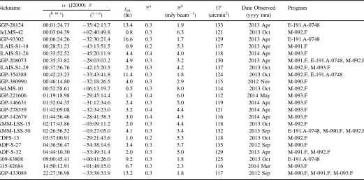
sampled map over the full 11′ diameter field of view of LABOCA. An average time of tint≈4.6 hr was spent integrating on each target (see Table 1). Maps with longer integration times(tint10 hr)provide deeper data sensitive to less luminous DSFGs in the vicinity of our signposts. Our shallower maps (tint1 hr) help constrain the abundances of the brightest DSFGs, thus reducing the Poisson noise associated with these rare galaxies. These deep/shallow 870μm data are necessary to constrain the photometric redshifts of the brighter/fainter DSFGs within the vicinities of our signposts, therefore allowing us to identify members of any candidate protocluster found.
During our observations, we recorded typical precipitable water vapor(PWV)values between 0.4 and 1.3 mm, corresp-onding to a zenith atmospheric opacity ofτ=0.2–0.4. Finally, the flux density scale was determined to an rms accuracy of σcalib≈7% using observations of primary calibrators, Uranus and Neptune, while pointing was checked every hour using nearby quasars and found to be stable toσpoint≈3″(rms).
2.3. From Raw Timestreams to Maps
The data were reduced using the Python-based BOlometer data Analysis Software package (BOA V4.1—Schuller 2012), following the prescription outlined in Section 10.2 and Section 3.1 of Siringo et al. (2009) and Schuller et al. (2009), respectively. We briefly outline the reduction steps below.
1. Timestreams for each scan were calibrated onto the
-Jy beam 1scale using primary or secondaryflux density
[image:3.612.46.567.76.333.2]calibrators. Table 1
Targets and Their Properties
Nickname α (J2000) δ tint ta sb Ωc Date Observed Program
(h m s) (°′ ″) (hr) (mJy beam-1) (arcmin2) (yyyy mm)
SGP-28124 00:01:24.73 −35:42:13.7 13.4 0.3 1.9 133 2013 Apr E-191.A-0748 HeLMS-42 00:03:04.39 +02:40:49.8 0.8 0.3 6.3 121 2013 Oct M-092.F SGP-93302 00:06:24.26 −32:30:21.4 16.6 0.3 1.7 129 2013 Apr E-191.A-0748 ELAIS-S1-18 00:28:51.23 −43:13:51.5 0.9 0.2 5.3 117 2013 Apr M-091.F ELAIS-S1-26 00:33:52.52 −45:20:11.9 4.4 0.4 4.0 118 2014 Apr M-093.F
SGP-208073 00:35:33.82 −28:03:03.2 4.9 0.3 3.2 130 2013 Apr M-091.F, E-191.A-0748, M-092.F ELAIS-S1-29 00:37:56.76 −42:15:20.5 2.9 0.3 4.2 137 2013 Oct M-092.F, M-093.F
SGP-354388 00:42:23.23 −33:43:41.8 11.4 0.3 1.8 124 2013 Oct M-092.F, E-191.A-0748 SGP-380990 00:46:14.80 −32:18:26.5 4.0 0.3 2.9 115 2012 Nov M-090.F
HeLMS-10 00:52:58.61 +06:13:19.7 0.5 0.3 8.0 114 2013 Oct M-092.F SGP-221606 01:19:18.98 −29:45:14.4 1.3 0.4 6.0 112 2014 May M-093.F SGP-146631 01:32:04.35 −31:12:34.6 2.4 0.3 5.0 119 2014 Apr M-093.F SGP-278539 01:42:09.08 −32:34:23.0 3.2 0.4 4.4 121 2014 Apr M-093.F SGP-142679 01:44:56.46 −28:41:38.3 3.0 0.4 4.3 116 2014 Apr M-093.F XMM-LSS-15 02:17:43.86 −03:09:11.2 2.0 0.3 4.4 118 2013 Oct M-092.F
XMM-LSS-30 02:26:56.52 −03:27:05.0 4.1 0.3 3.4 132 2013 Sep E-191.A-0748, M-090.F, M-092.F CDFS-13 03:37:00.91 −29:21:43.6 1.0 0.2 5.3 118 2013 Oct M-092.F
ADF-S-27 04:36:56.47 −54:38:14.6 3.4 0.3 3.7 135 2012 Sep M-090.F ADF-S-32 04:44:10.30 −53:49:31.4 2.0 0.3 5.0 129 2013 Apr M-091.F, M-092.F G09-83808 09:00:45.41 +00:41:26.0 9.2 0.3 1.8 125 2013 Oct E-191.A-0748 G15-82684 14:50:12.91 +01:48:15.0 6.7 0.3 2.3 116 2014 Mar M-093.F
SGP-433089 22:27:36.98 −33:38:33.9 13.2 0.3 1.8 117 2012 Sep M-090.F, M-091.F, M-093.F
Notes.Targets are listed in order of increasing R.A.
a
Average opacity value.
b
Average depth computed across each beam-smoothed LABOCA map, where the resulting FWHM of a beam is 27″.
c
Extent of LABOCA map.
21
http://hedam.oamp.fr/hermes/
22ESO program E-191.A-0748 and MPI programs 090.F-0025-2012,
M-091.F-0021-2013, and M-092.F-0015-2013.
2. Channels exhibiting strong cross talk with their neigh-bors, showing no signal or high noise wereflagged, while the remaining channels were flatfielded.
3. Timestreams wereflagged in regions where the speed and acceleration of the telescope are too severe to guarantee reliable positional information at every timestamp. 4. In an iterative manner, the following sequence was
performed:
(a)Noisy channels were σ-clipped relative to all channels with the degree of clipping increasing from 5 to 3 with each iteration.
(b)Sky noise determined across all channels was removed from each channel.
(c)Each channel’s timestreams were “despiked” about their mean value.
(d)An nth-order polynomial baseline was subtracted from the timestreams to remove any low-frequency drifts, where n=1–4 with each iteration.
5. Large discontinuities(jumps)in the timestreams, seen in all channels, and correlated noise between groups of channels (e.g., channels sharing the same part of the electronics or being connected to the same cable) were removed.
6. The Fourier spectrum of the timestreams were high-pass filtered below 0.5 Hz using a noise-whitening algorithm to remove the 1/f noise. At this stage, the mean noise-weighted point-source sensitivity of all channels was calculated to remove scans corrupted by electronic interference. Uncorrupted scans were opacity-corrected using skydips and radiometer opacity values before being pixelated onto a map. We oversampled the pixelization process by a factor of four to preserve the spatial information in the map. This results in afinal map for a given scan with a pixel scale p≈4 8 pix−1.
We coadded, with inverse weighting, all of the reduced maps for each scan before beam smoothing thefinal map to ease the detection of point sources and to remove any high-frequency noise on scales smaller than the beam that might exist. The effect of convolving with a Gaussian with a FWHMθ=19 2 (i.e., the beam width, see Figure 1) increase the spatial resolution to q2+q2 = 2q»27. Thus we scale thefinal
map by 2 in order to preserve the peak intensity, i.e., the mJy beam−1units. As our rms maps are also smoothed by a 19 2 Gaussian, we applied an additional scaling to them such that the signal-to-noise ratio (S/N) in regions free of sources was unity.
We repeated these reduction steps, this time using the final reduced map as a model to mask significant sources before flagging the timestreams. Using a model in this fashion helps to increase thefinal S/N of detections(Nord et al.2009; Schuller et al.2009; Belloche et al.2011). Wefind that one repetition is sufficient to achieve convergence in the S/N of a point source, in agreement with the findings of Weiß et al. (2009) and Gomez et al.(2010). We present thefinal S/N maps for all of our ultra-red galaxies in AppendixA.
To model the instrumental noise of our maps, we generated so-called “jackknife”maps by randomly inverting(i.e., multi-plying by−1)half of our reduced scans before coadding them. The result is a map free of astronomical sources and confusion, which we estimate to be »0.9 mJy in our deepest maps, and thus these realizations will underestimate the true noise. For
each map, we created 100 jackknife realizations of the instrumental noise.
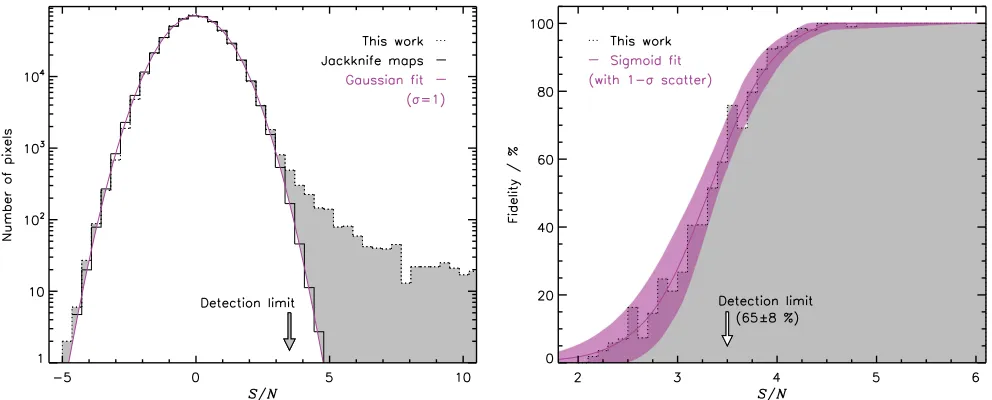
In Figure2we show the pixel distributions of thefinal S/N maps and their respective jackknife realizations. There is clearly a positive excess above S/N3 in the final reduced maps compared to the jackknife maps. This excess is caused by the presence of astronomical sources.
3. Analysis
We chose a detection threshold(Σthresh)based on the values of a“fidelity”or“trustworthiness”parameter,, similar to that outlined in Aravena et al.(2016). For all of our maps, we ran our extraction algorithm (Section 3.1) and compared the number of sources detected in our maps, , to the mean number of sources detected in our 100 jackknife realizations for each map, jack, as a function of detection S/N:
= -1 jack. ( )1
We show the average fidelity in the right-hand panel of Figure2, which illustrates that by increasing the detection S/N, we increase our confidence in the recovered sources. We reach afidelity of»100%at5σ and afidelity of=50% at ≈3σ, the latter indicating that we would expect about half of our sources to be spurious at S/N≈3. We chose—as a compromise between reliability and the number of cataloged sources—a detection threshold ofΣthresh>3.5, where we have afidelity»658%.
The intrinsic map-to-map scatter in thefidelity is caused by the varying abundance of sources in each map, due to the effects of cosmic variance and the differing rms noise levels. This scatter decreases with increasing detection threshold and is
[image:4.612.321.565.50.250.2]s » 3%at 5σ.
Figure 1.Main: Radially averaged beam profile of J2258−280, the most frequently visited pointing source for this work, reduced in the same manner as our maps. Black points indicate radial bin averages and their respective rms values, after sky subtraction. The beam is well described by a Gaussian with FWHMθ=19 2(purple line), which we use to beam-smooth ourfinal maps. Inset: Normalized flux map of J2258−280 (Sn=765.426.2 mJy)
with contours indicating the 10, 30(black), 50, 70, and99 white %( ) peak
3.1. Source Extraction
We used a custom-written Interactive Data Language(IDL—
Landsman 1993) source-extraction algorithm to identify and extract sources in the beam-smoothed S/N maps, noting that the beam-smoothing step described above optimizes the detection of point sources.
In a top-down fashion, we searched for pixels above our floor S/N detection thresholdΣthresh>3.5σ. To accommodate sources whose true peak falls between pixels, we temporarily lowered Σthresh by ≈95%, keeping sources with bicubically interpolated sub-pixel values that meet our original S/N detection threshold. In Table 5 we catalog the peak flux density, noise, and position determined from a three-parameter Gaussianfit made inside a box of widthθ(i.e.,≈27″)centered on a source. After removing thefit from the map, we searched for and cataloged subsequent peaks until no more could be found.
During the extraction process we performed some additional steps: the parameters of sources deemed too close to each other (Δr<θ/2) were reevaluated by fitting multiple three-para-meter Gaussians simultaneously; sources deemed too close (Δr<θ/2)to the map edges were rejected.
3.1.1. Completeness, Flux Boosting, and Positional Offsets
We inserted simulated sources into our jackknife maps to quantify the statistical properties of our cataloged sources. To ensure that we did not encode any clustering, we randomize the injection sites of our simulated sources. We drew model flux densities down to Smod=1 mJy from a Schechter function
parameterization of the number counts,
µ
a
-⎛ ⎝
⎜ ⎞
⎠
⎟ ( )
dN dS
S
S e , 2
S S
mod
mod 0
mod 0
where S0=3.7 mJy and α=1.4(Casey et al. 2013), which
we scaled to 870μm using a spectral index of ν2, i.e., we divided the modelfluxes by(ν870/ν850)2≈1.05.
For each simulated source, we ran our source-extraction algorithm, and if we detected a peak within a threshold radius,
´q
rthresh 1.5 , of the injection site, then we recorded the
best-fitting Gaussian parameters. If we recovered multiple peaks within our threshold radius, we took the most significant. Finally, if we failed to recover a simulated source, we recorded the model flux density and the instrumental noise at the injection site.
This procedure was repeated 10,000 times for each target so that we generated a large, realistic catalog of simulated sources. We used this to determine the noise-dependent completeness, , i.e., the fraction of recovered sources to input sources, as well as theflux boosting,, i.e., the ratio of recovered to input flux densities, and the radial offsets, , i.e., the distance between recovered and input positions for each cataloged source.
We calculated the medianflux boosting in bins of recovered S/N, which we used to translate the recoveredflux densities of our detections into model flux densities (see Figure 3). After this stage, we used our deboosted flux densities with their associated instrumental noise levels to determine their completenesses and radial offsets. The former we computed from a spline interpolation of a two-dimensional surface of modeledflux density and instrumental noise(see Figure4and, e.g., Geach et al.2013), while the latter we computed from a spline interpolation of modeled S/N (see left-hand panel of Figure5).
At our detection threshold, theflux density of a source in our deepest map, SGP-93302, is typically boosted by =1.7, which is in agreement with the literature at similar depths(e.g., »1.5—Geach et al. 2017), while at S/N6, the flux boosting becomes negligible. However, we draw attention to the relatively severe deboosting factors recorded for our noisiest maps (e.g., central rms, s5 mJy for SGP-221606) due to the steep bright-end(Sn >13 mJy)slope of the number counts.
[image:5.612.59.555.51.251.2]For SGP-93302, our two-dimensional completeness function indicates that we are »100% complete at a deboosted Figure 2.Left: Beam-smoothed S/N pixel distribution for our maps(dotted, black histogram)that shows an excess above our detection threshold due to the presence of astrophysical sources(gray region). We also plot the beam-smoothed S/N pixel distribution of our jackknife maps(black solid histogram, see Section2.3), whose mean is well modeled by a Gaussian(solid, purple line)centered onμ=0 with a standard deviationσ=1, as expected. Right: Meanfidelity(black, solid histogram
—)as a function of detection S/N for our maps using our extraction algorithm(see Section3.1). We parameterize the histogram by a sigmoid function(purple, solid line), which we use to deduce thefidelity of each source detected. We draw attention to the fact that this is a statistical measurement and that on average 65±8% of sources detected at 3.5σwill be trustworthy, i.e., a third of these sources may be spurious.
flux density and instrumental noise of Smod»5 mJy and
sinst»1.2 mJy, respectively. In this same flux density plane,
our completeness falls close to »0% as the instrumental noise reachessinst»2.5 mJy.
In the left-hand panel of Figure5we see that the mean radial offset is in good agreement with that expected from Equation (B22)in Ivison et al.(2007). There exists a large scatter in the low S/N5 bins, which indicates that our radial offsets at a given S/N value can vary by as much ass= 2. 5. We also
note that our brightest detections with S/N≈30 have radial
offsets as little as= 0. 5, allowing us to accurately constrain the positions of such sources.
Finally, the simulated sources that we successfully recovered match the Schechter source counts given in Equation (2) to within 1σ, with no underlying systematics remaining.
3.2. Herschel SPIRE Photometry
In order to derive photometric redshifts for the LABOCA-detected DSFGs, we bicubically interpolated the SPIRE fl ux-density maps at the LABOCA source positions. We determined the errors and local sky values from a box of width≈12×θSPIRE centered on each detection, whereθSPIRE≈18″, 24″and 35″for the 250, 350 and 500μm passbands, respectively (Valiante et al.2016).
To quantify the effect that the LABOCA radial offset has on determining our SPIRE measurements, we analyzed how the “true flux density” of a source varied as we tweaked the position at which we measured it. For each survey field and passband, we selected a bright (S250≈S350≈S500≈ 1 Jy) point source and measured the true flux density at its cataloged position. We then performed 500 Monte Carlo simulations, drawing radial offset values from a Gaussian distribution centered on the cataloged position with a standard deviation23 s=, which we allowed to range across =
–
0 10 . For each simulation, we measured theflux density at the adjusted positions and compared them to the true flux density. We used this ratio (Frec) to flux-boost a SPIRE photometric measurement, depending on the LABOCA radial offset it exhibited. We parameterize this value using Frec %=100
- ab
( ) , whereα=1.0, 1.4, and 1.9 andβ=1.7, 1.8, and 1.9 at 250, 350, and 500μm, respectively.
The right-hand panel of Figure 5 shows that the average radial offset is passband related, reflecting the different pixel scalings of 6″, 8 3 and 12″pix−1for the 250, 350, and 500μm passbands in H-ATLAS, respectively (similar values are recorded in HerMES). We see that for detections with low radial offsets, < 2 , and thus high S/N8 values, we recover ≈95% of the true flux density. Owing to the large SPIRE 500μm pixel size, even at the highest radial offsets considered in this paper(»10)for sources near to or at our detection threshold, we still recover 80% of the true flux density. Conversely, however, we only recover 55% and
65% of the trueflux densities for these highest offsets at 250 and 350μm, respectively.
[image:6.612.48.291.49.254.2]We draw attention to 16 (i.e., ≈15%) of our LABOCA sources that are undetected at the 1σlevel in all SPIRE maps. The majority (12) of these possibly spurious sources have detection S/N4.5, in agreement with our fidelity analysis. The number of sources with higher S/N values is also expected when the intrinsic scatter in thefidelity parameter is taken into account. These sources do not affect our number counts because on average, we correct for this effect. Thus ourfidelity =658%and highflux-boosting factors at these low S/N thresholds weights these possibly spurious sources accordingly. However, we choose not to include any of these sources in our photometric redshift analysis—we are unable to meaningfully constrain them.
Figure 3.Flux boosting(i.e., recovered vs. modeledflux density)as a function of recovered S/N for SGP-93302. We generate a model flux density distribution using the Schechter parameterization of the number counts given in Casey et al. (2013) when determining these corrections. We record a negligibleflux-boosting factor,<1.1, at S/N6.0 and witness corrections of »1.7 at our detection threshold, comparable to that of S2CLS (»1.5—Geach et al.2017), despite the different noise levels.
Figure 4.Completeness for SGP-93302 as a function of instrumental noise and modelflux density. The two-dimensional treatment of our completeness is vital due to the radially varying sensitivity across our maps. We see that as the instrumental noise decreases and our model flux density increases, our completeness increases as well. For this map, at an instrumental noise and model flux density ofsinst»1.2 mJy and Smod»1 mJy, respectively, we
recover hardly any sources, i.e.,»0%. However, increasing the modelflux density to5 mJywhile keeping the noise constant results in most sources being recovered successfully, i.e.,»100%.
23
[image:6.612.49.288.346.523.2]Finally, we note that the SPIRE fluxes derived in this manner, i.e., using a LABOCA prior and a radial offset fl ux-boosting value, are consistent with those from which they were originally selected—varying by±1σ.
3.3. Photometric Redshifts
We use a custom-written χ2-minimization routine inIDLto determine far-IR-based photometric redshifts for our catalog of sources, which have at least one SPIRE detection above
>1σSPIRE. We fit to three well-sampled spectral energy distributions (SEDs) used in Paper I: that of the Cosmic Eyelash (Ivison et al. 2010; Swinbank et al. 2010), and synthesized templates from Pope et al. (2008) and Swinbank et al. (2014), ALESS. Figure 4 in Paper I highlights the diversity of these SEDs in the rest frame, each normalized in flux density atλrest=100μm.
We use the deboosted 870μm and boosted SPIRE flux densities during our template fitting. The fitting is done in linear space (accommodating for negative fluxes) over a photometric redshift range0<zphot<10down to a resolution
of Δz=0.01. We adopt the photometric redshift associated with the template that produces the overall minimumχ2value (cmin2 )and report 1σerrors based on thec +
1
min
2 values. We
find that the errors determined in this way are consistent with the Monte Carlo method used in Paper I. However, they are inconsistent with the intrinsic scatter deduced from a training sample of spectroscopically confirmed DSFGs that meet our ultra-red criteria. In Paper I, we find that the accuracy and scatter in Dz (1 +zspec)=(zphot-zspec) (1 +zspec) are mDz= -0.03 1( +zspec) and sDz=0.14 1( +zspec),
respec-tively. This scatter is representative of the minimum systematic uncertainty when determining photometric redshifts using these three templates—significantly larger than that determined from both thecmin2 +1values at high redshift.
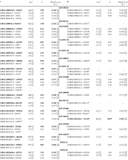
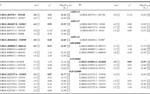
The results of thesefits, as well as the rest-frame 8–1000μm luminosities are presented in Table4.
4. Discussion
We catalog 108 DSFGs from our 22 maps above
Σthresh>3.5 and list their SPIRE and LABOCAflux densities and their mean flux boosting, , and mean fidelity, , parameters in Table5. Our signpost ultra-red galaxies span a deboosted flux density range ofS870=2.9 42.8 mJy– , with a mean S870=17.0 mJy. The surrounding field galaxies span
a deboostedflux density range ofS870=1.9 31.3 mJy– with a meanS870=6.8 mJy. There are two exceptionally bright, new
DSFGs with S87025 mJy, but on average, the new field
galaxies are less bright than our target ultra-red galaxies. We are unable to detect four of our target ultra-red galaxies above our S/N>3.5 threshold; all of these are located in our shallower maps. In such cases, we report the peakflux and rms pixel value within a 45″ aperture centered on the telescope pointing position. We do not provide completeness, fl ux-boosting,fidelity, or radial offset values for these sources.
4.1. Number Counts
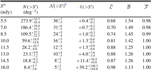
We deduce number counts, which we list in Table 2 and display in the left-hand panel of Figure6, using the following equation:
å
> ¢ = " > ¢
( ) ( )
N S , 3
Si S
[image:7.612.60.557.52.254.2]where the sum is over all deboostedflux densities,Si, greater than some thresholdflux,S¢. Fidelity corrections,, are made using the detected S/N values, while completeness corrections, , are made using the deboostedflux densities and instrumental noises. The area surveyed at a recovered flux density, , is obtained by cumulating the area across all of our maps where a givenflux density is detected above our threshold. These three corrections account for the varying map rms values in our sample.
We exclude the target ultra-red galaxies to partially remove the bias associated with imaging a region where a galaxy is already known to reside. We note, however, that this method does not fully remove all of the bias associated with imaging a region centered on a galaxy. The reason is that galaxies themselves are known to cluster(Greve et al.2004; Weiß et al. 2009). Thus, these “galaxy-centric” regions will be, by definition, overdense relative to arbitrarily selected regions.
The errors on the number counts are deduced using
s = > ¢ s
> ¢
> ¢ ( )
( ) ( )
( ) N S
S , 4
N S G86
where σG86 are the double-sided 1σ Poisson errors (Gehrels 1986) and (> ¢S) are the number of sources above each thresholdflux density.
Because of the largeflux density uncertainties in some of the cataloged DSFGs, we compare the method outlined above to drawing realizations of the flux densities and computing Equation (3) for each realization, adjusting , and accordingly. We then take the median and errors from the 15th and 84th percentiles from the median. We find no significant variation in the results obtained from either method, which suggests that the largeflux density uncertainties do not severely affect our number counts analysis.
Our number counts are always 1σ above those from the LABOCA Extended Chandra Deep Field South (ECDFS) Submillimetre Survey (LESS—Weiß et al. 2009) and the
SCUBA-2 Cosmology Legacy Survey (S2CLS—Geach
et al. 2017). We see a slight break in the shape of counts at
¢ >
S 7 mJy, similar to that seen in the LESS number counts. Figure6 shows that there are similarities in the shape of our number counts to those of J2142−4423, a Lyα protocluster (Beelen et al.2008), atS¢7 mJyandS¢14 mJy. However, it is unclear whether Beelen et al. (2008) removed the target source from their number counts, which, as mentioned earlier, will bias their results higher. Furthermore, Beelen et al.(2008) claim that the environments around J2142−4423 are only moderately overdense compared to SHADES—but as discussed previously, we believe this to be evidence that J2142−4423is overdense compared to LESS and S2CLS. Figure6also shows the number counts of MRC 1138262(the so-called“Spiderweb
galaxy”—Miley et al.2006; Dannerbauer et al.2014), a HzRG with an overdensity of sources compared to LESS atS¢ >7 mJy (i.e., ≈385 deg−2). This protocluster is ≈2×more overdense compared to our work, but it should be noted that Dannerbauer et al. (2014) neither account for flux boosting nor survey completeness, nor do the authors remove the target galaxy (DKB07). We crudely correct for the first two of these differences using the results obtained for SGP-93302, which was observed under similar conditions for a similar integration time to MRC 1138262. Adjusting for these corrections, we record less extreme number counts of N(>6 mJy)≈394± 176 deg−2 (1σ Poisson errors) that exhibit a sharp break at
¢ »
S 6.5 mJy. Thus, MRC 1138−262 has number counts that are only slightly higher than those presented in this work.
In Figure 7 we show how the contribution to our number counts at the flux densities provided in Table 2 varies in two signpost-centric annuli of equal area(16πarcmin2). We see that at S¢ > 8.5 mJy, ≈80% of the contribution to the number counts comes from DSFGs distributed withinrtarget< ¢4 of our
signposts. However, because of the low numbers of galaxies above these deboosted flux-density thresholds, this excess contribution is not significant(≈1.5σ). However, the increasing instrumental noise with distance from our signposts causes comparisons of the number counts at all but the highest flux densities to become heavily biased. We see that at the higher flux-density thresholds, this perceived excess diminishes rapidly, and aboveS¢ >11.5 mJy, the contribution appears to be equally split between the two annuli. Thus, without uniformly wide imaging of these environments, the number counts as a function of radial distance remain largely unconstrained for this sample.
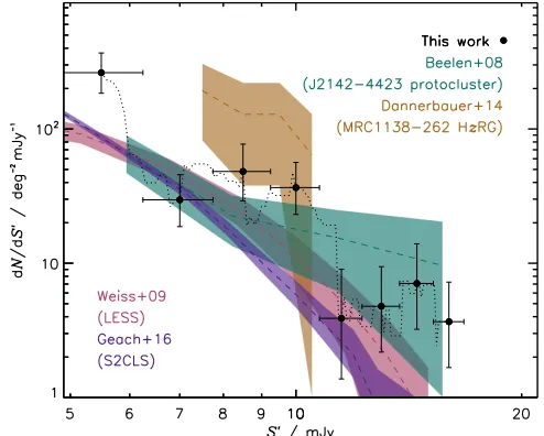
Finally, in Figure8we show the differential number counts for this work alongside those of the LESS and S2CLS blank fields and the two known protoclusters J2142−4423 and MRC 1138262.
4.2. Overdensities
In order to make a statistical analysis of the significance of our number counts, we employ an overdensity parameter (Morselli et al.2014)
d > ¢ = > ¢ > ¢
-( ) ( )
( ) ( )
S N S
N S blankfield 1, 5
where N(> ¢S)blankfield are the number counts expected in a
blank-field survey above some thresholdflux density.
[image:8.612.42.296.74.196.2]When choosing a blank-field survey suitable for comparison, it is important to compare“like-for-like”(i.e., Condon 2007). For instance, broad-beam surveys can hide the multiplicity of DSFGs; multiplicity wasfirst identified in early interferometric observations with the Very Large Array(VLA)/SMA/Plateau de Bure Interferometer(PdBI; e.g., Tacconi et al.2006; Ivison et al.2007; Biggs et al.2011; Wang et al. 2011; Barger et al. 2012; Smolčićet al.2012), confirmed for large samples using ALMA observations(Karim et al.2013; Bussmann et al.2015; Simpson et al.2015; Oteo et al.2017a), and is consistent with models of galaxy formation (e.g., Smolčić et al. 2012, Narayanan et al.2015). Furthermore, similar—if not identical —data reduction techniques ensure consistency in the flux densities and associated errors, which may otherwise lead to a lower or higher estimate of the number counts (see Section4.2.1).
Table 2
Number Counts and Overdensities
S′a N(> ¢S) (> ¢S)b d(> ¢S)
(mJy) (deg-2)
5.5 273.9-+45.453.7 36-+75 +0.4-+0.10.1 0.68 1.54 0.98
7.0 186.4-+33.339.9 31-+65 +0.7-+0.20.2 0.70 1.49 0.98
8.5 109.5-+22.227.2 24-+54 +1.0-+0.30.3 0.74 1.45 0.99
10.0 59.6-+14.818.9 16-+35 +1.3-+0.50.6 0.81 1.42 1.00
11.5 28.2-+8.010.7 12-+43 +1.5-+0.80.9 0.88 1.25 1.00
13.0 23.1-+7.29.9 10-+43 +4.0-+3.43.6 0.88 1.26 1.00
14.5 18.8-+6.59.3 8-+32 +11.4-+16.016.5 0.87 1.26 1.00
16.0 8.4-+3.65.7
-+
5 23 +39.2-+144.8146.3 0.98 1.13 1.00
Notes. a
Flux-density threshold levels are taken from Weiß et al.(2009)to simplify the comparisons we made with LESS.
b
Hence, we choose the LESS number counts (calculated directly from the source catalog)to make comparisons. These data and ours were obtained from the same instrument and are reduced in a similar manner using the same software. However,
[image:9.612.61.556.50.251.2]there are slight differences in the results when we run our source-extraction algorithm on the LESS DR1.0 S/N map.24 Using a detection threshold ofΣthresh>3.7, we recover 95% of their sources. Our 870μm flux density measurements are Figure 6.Left: Number counts(excluding our target ultra-red galaxies)as a function of 870μmflux density(black circles)with 1σdouble-sided Poisson errors (Gehrels1986). We show the blank-field number counts from LESS(pink region)and S2CLS(purple region—scaled with a spectral index ofν2)surveys. We also show the number counts of two known protoclusters, J2142−4423(green region—Beelen et al.2008)and MRC 1138262(brown region—Dannerbauer et al.2014). It is clearly evident that our number counts are high at allflux density thresholds and exhibit a slight break atS¢ >7 mJy. We believe that the increasing excess at higher
flux densities is the result of our ultra-red galaxies signposting similarly extreme DSFGs. Our catalog containsfive bright(S870>16 mJy)sources. However, we
[image:9.612.319.566.376.574.2]concede that we are unable to rule out gravitational lensing by chance alignment as a cause for the bright sources without high-resolution imaging. Right: Number counts relative to LESS, i.e., the overdensity parameter,d(> ¢S). In black we show the results for the entire sample(i.e., the circles from the left-hand panel), while in colored circles we show the overdensity for each map. The size of each circle has been logarithmically scaled to show the influence that each target has in deducing the number counts for the whole sample. Maps where no sources are present above a given thresholdflux are indicated by staggered squares starting fromδ<−1 for clarity. These squares highlight the deficit of sources due to intrinsic properties(i.e., cosmic variance)and varying map rms values. Hence, we see that some maps probe considerably more overdense regions than others, with variations being sometimes as high≈×5. Finally, we color-code each target from blue to red in order of increasing R.A., i.e.,in the order that our targets appear in Table1and the color that they have in Figure13.
Figure 7.Contribution to the cumulative number counts from two signpost-centric annuli with equal area(i.e., 16πarcmin2). We separate each annuli by
dashed black lines and divide them into eight equally sized segments representing the 870μmflux-density thresholds listed in Table2. We color-code the contribution to the total number counts from each annuli in a given segment(see scale). AtS¢ <8.5 mJy, we see that the inner annuli contributes ≈80% of the sources responsible for the total number counts. However, by
¢ >
S 11.5 mJy, the contribution is equally split between the two annuli, within the large Poisson errors(σ≈30%). This highlights the difficulty in claiming any radial dependence on the number counts due to variations in the instrumental noise(i.e., the noise increases as the distance from our signposts increases).
Figure 8.Differential number counts(excluding our target ultra-red galaxies) as a function of 870μmflux density(black circles). As in Figure6, we also show the differential number counts for the LESS(pink)and S2CLS(purple) blankfields as well as the two known protoclusters J2142−4423(green)and MRC 1138262 (brown). We see that above S¢ >8.5 mJy, our differential number counts are typically 1σgreater than those presented in LESS—our comparisonfield of choice.
24http://archive.eso.org/cms/eso-data/data-packages/
less-data-release-v1-0.html
[image:9.612.48.292.376.559.2]comparable to those in Weiß et al.(2009)as we record a mean absolute offset of∣DSn∣=0.4 mJy. These differences should have a relatively minor effect on comparisons made with the number counts. However, the computation of completeness and flux-boosting parameters do differ. We record 15% differ-ences in the latter at a detection S/N≈3.7 for sources around SGP-433089, which has a similar (although slightly higher) average depth to LESS. We note that Weiß et al.(2009)claim that LESS is underdense and also shows a deficit of bright sources relative to other blankfields. However, Figure6shows that this is clearly not case when adopting the much deeper and wider data from S2CLS as a reference.
We make overdensity comparisons at aflux-density thresh-old of S¢ > 8.5 mJy, which equates to a surveyed area of »0.2 deg2at our detection threshold. We choose thisfl
ux-density threshold to be directly comparable to LESS. Furthermore, this threshold is high enough to minimize the correction effects needed for our low S/N detections. At the same time, it is low enough such that our results should not drastically change if our bright sources are magnified byμ2. We add our number-count error bars in quadrature to those given in Weiß et al. (2009). We determine an overdensity of d= -+
1.0 0.3
0.3 at S¢ >
8.5 mJy. In other words, we are 99.93% confident that our signposts pinpoint overdense regions in the universe, and we are≈95(50)% confident that these regions are overdense by a factor of at least 1.5(2)×compared to LESS. However, we stress that byonlyremoving the target galaxy from our number counts analysis, we are left with a “residual bias” due to imaging a region where a galaxy is known to reside. We estimate that this residual bias increases our overdensity parameter by dresid. bias=0.230.02 over the
typical map areas (p(6.2-+0.10.3 2) ) that we have surveyed in
this work.
Furthermore, we crudely test what effect removing sources with S/N4 and S/N4.5 has on this overdensity calculation. This S/N regime is close enough to our detection threshold such that the completeness corrections and surveyed area values that we apply should be similar. Thus, we derive overdensity values of δ=1.0±0.3 and δ=0.7±0.2 for sources with S/N>4 and S/N>4.5, respectively. This suggests that despite a non-negligible fraction of sources near our detection threshold potentially being spurious, our over-density above 8.5 mJy is comprised of secure LABOCA detections.
Finally, we test the effects that cosmic variance has on our ultra-red galaxies and our comparisonfield of choice, LESS. To do this, we simulate 100 2 deg×2 deg images, which we populate with clustered sources—governed by the observed two-point angular correlation function given in Weiß et al.(2009).
For each ultra-red galaxies, we extract a randomly placed sub-image from 22 randomly chosen simulated images, each with an area that matches our LABOCA data given in Table1. We then calculate the number of sources present in these sub-images and repeat this process 1000 times. The standard deviation of the total number of sources in each of these 1000 repetitions incorporates, in quadrature, the Poisson noise and the noise from cosmic variance, which we estimate to≈15% on the ultra-red galaxy number counts.
For LESS, we extract a randomly placed, LESS-sized sub-image from each of these larger simulated sub-images and compute
the standard deviation—deriving a relative error of≈20% on the LESS number counts.
As both of the effects from cosmic variance are weaker than that accounted for in the Poisson noise (≈40% and ≈50%, respectively), we do not propagate either into the error budget for our overdensity parameter.
There exists a strong correlation in flux density with our overdensity parameter, as seen in the right-hand panel of Figure 6. Here we plot the overdensity parameter for each target, which we have logarithmically scaled to reflect each target’s contribution to our overall number counts. We see a large scatter across our 22 maps, which is indicative of cosmic variance and varying levels of map noise. The evolution in overdensity increases ∼50×from S¢ =7 16 mJy– , although the Poisson error from the blank-field counts rises steeply at the higherflux densities, exacerbated by the large relative error in the number counts of bright sources in LESS. We believe that this evolution is caused by our ultra-red galaxies signposting regions that contain brighter DSFGs. However, without high-resolution imaging of the environments around our ultra-red galaxies, we cannot rule out gravitational lensing by chance alignment.
4.2.1. Mundane, Not Cosmic, Underdensity in LESS
It is often claimed that LESS exhibits an underdensity of DSFGs—resulting in the introduction and use of(Dannerbauer et al. 2014; Swinbank et al. 2014) a multiplicative “ fudge-factor”(∼2×)to the number counts presented in Weiß et al. (2009). An“adjustment”of this magnitude would require us to significantly lower the value of the overdensity parameter, if necessary.
This perceived underdensity is concluded against the number counts presented in SHADES (SCUBA HAlf Degree Extra-galactic Survey—Coppin et al.2006)as it was the largest“ like-for-like” survey at the time. Recently, the Subaru/ XMM-Newton Deep Field (SXDF)—one of the two extragalactic fields in SHADES—has been reimaged during the S2CLS, which has improved the sensitivity of thisfield by2×.
Using these new data, however, we are only able to match 27/60(45%)of the SXDF detections25to a counterpart in the S2CLS.26 These “matched” sources have typical offsets of 4 7±3 0 and deboosted flux densities that are on average (1.6±0.1)×greater than those reported in the S2CLS. The 33/60 (55%) “unmatched” detections have a broad range of deboostedflux densities,S=3.1–22.0 mJy. These values from SHADES are typically≈4×higher than the measurements we make at their respective positions in the S2CLS image.
Thus, if these results were to be replicated for the Lockman Hole East—the second extragalactic field in SHADES—it would appear that the spurious fraction of sources and/orfl ux-boosting corrections have been miscalculated. Taken together, these findings suggest that the claimed underdensity in LESS and apparent deficit of bright DSFGs is unlikely to be true and unlikely to be biasing the overdensity parameter of our ultra-red galaxies. Furthermore, thesefindings are very reminiscent of those discussed by Condon (2007), who resolved the inconsistencies amid differing reports of the radio number counts at the time. Thus, in homage, the variance in the number counts between SHADES and LESS appears to be“mundane” 25
http://www.roe.ac.uk/ifa/shades/dataproducts.html
26
(likely due to instrumental and analysis effects) rather than “cosmic.”
4.2.2. Probability of Being Ultra-red
As can be seen Table 5, half of our signposts have SPIRE photometry, which is just consistent with them being ultra-red. This motivates us to derive for thefirst time a probability that a galaxy is actually ultra-red (PUR) based on its SPIRE photometry.27 To this end, we draw 10,000 realizations of the SPIRE photometry from a Gaussian distribution and determine the number of times that these realizations meet our ultra-red criteria outlined in PaperI. By incorporating the photometric errors from all SPIRE bands, we are able to generate a subset of galaxies that are likely to be ultra-red. Finally, we derive 1σ errors assuming Poisson statistics for these ultra-red galaxy probabilities, which we list in Table 3.
In Figure 9we show how the overdensity parameter above
¢ >
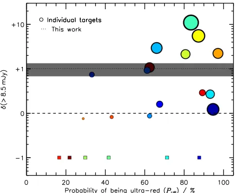
S 8.5 mJy varies as a function of its probability of being ultra-red for our signposts. Clearly, galaxies that have a higher probability of being ultra-red typically have a much higher overdensity parameter. Furthermore, overdense signposts(i.e., signposts withδ>0)all have a probability of being ultra-red greater than PUR30%. This lower limit value is caused by
galaxies lying at the boundaries of both of our SPIRE color cuts outlined in Paper I. Above a probability of being ultra-red of
PUR 60%, we see that only three (≈20%)of our signposts
have environments that are consistent with being underdense (i.e.,δ<0). Such a low fraction of underdense environments suggests that using this novel ultra-red-probability technique in
conjunction with 870μm imaging provides a robust method for signposting overdensities in the distant universe.
4.3. Colors
We analyze theS500 S250and S500/S350colors to see if our field galaxies comprise similarly red galaxies as our signposts. We recall that in the further analysis we exclude 16 LABOCA detections as we are unable to constrain their photometric redshifts. This leaves us with 86–16=70 DSFGs around our 22 ultra-red signposts above >3.5σ. Figure 10 illustrates that only 7%(≈5 DSFGs)of ourfield galaxies meet our ultra-red galaxy criteria. Such a low fraction might be expected as our ultra-red galaxy criteria select the most luminous and rare DSFGs. If we relax the 3.5σ500threshold(imposed in PaperI) to 1σ500, our fraction of field ultra-red galaxies increases to 17%(≈12 DSFGs)at the expense of being less reliable.
Our field galaxies have median S500/S250 and S500/S350 colors of(S500 S250 1 2) =1.1and(S500 S350 1 2) =0.9,
respec-tively, with interquartile ranges of S500 S250=0.7 1.4– and
S500/S350=0.7–1.2. If we isolate the field galaxies that we assume to be physically associated with their target galaxy(see Section 4.4), we note a redder change as theS500/S250 color increases to a median (S500 S250 1 2) =1.4 with interquartile
range S500 S250=1.2 1.5– . However, we see no appreciable change in theS500/S350color. As can be seen in Figure10, this can be explained by five signpost galaxies narrowly missing our original ultra-red criteria when their SPIRE photometry has been remeasured at their LABOCA position.
Thus, if we go one step further and isolate the associatedfield galaxies that contribute to the overdensity atS¢ >8.5 mJy, we find that they have redder median colors of(S500 S250 1 2) =1.0
and(S500 S350 1 2) =1.4. This is in part due to the exclusion of
[image:11.612.323.566.51.250.2]SGP−433089 and its associated galaxies, which—having had its SPIRE photometry remeasured at the position of its LABOCA Table 3
Targets and Their Probability of Being Ultra-red
Nickname PUR
(%)
SGP-28124 94.6±0.4
HeLMS-42 87.4±0.4
SGP-93302 67.5±0.2
ELAIS-S1-18 33.4±0.1
ELAIS-S1-26 61.4±0.2
SGP-208073 62.2±0.2
ELAIS-S1-29 65.8±0.2
SGP-354388 93.2±0.4
SGP-380990 71.1±0.3
HeLMS-10 83.6±0.3
SGP-221606 41.8±0.1
SGP-146631 29.9±0.1
SGP-278539 81.0±0.3
SGP-142679 87.5±0.4
XMM-LSS-15 29.5±0.1
XMM-LSS-30 97.1±0.4
CDFS-13 28.5±0.1
ADF-S-27 43.1±0.1
ADF-S-32 16.5±0.0
G09-83808 89.0±0.4
G15-82684 62.6±0.2
SGP-433089 21.7±0.0
[image:11.612.43.295.72.327.2]Note.Targets are listed in order of increasing R.A., i.e., in the same order as they appear in Table1.
Figure 9.Overdensity parameter aboveS¢ >8.5 mJyvs. the probability that our signposts are ultra-red using the method outlined in the text. Each target is color-coded and represented as a circle with a size reflecting its overall contribution to the number counts, i.e., as described in the caption of Figure6. The mean overdensity at thisflux-density threshold is shown as a black dotted line, while the shaded area represents its 1σ uncertainty. This shows that approximately half of our ultra-red galaxies havePUR68%once their SPIRE flux densities have been reevaluated at their LABOCA position. Conversely, signposts that have a higher probability of being ultra-red contribute more to the mean overdensity at thisflux-density threshold.
27
These probabilities are calculated by assuming symmetric color uncertain-ties, and do not take the bias into account that more bluer galaxies will have had their colors scattered redward, into the ultra-red category, than vice versa. However, these are only used as a guide to the likelihood of being ultra-red.
Table 4
Targets and Their Photometric Redshift Properties
ID zphota c2 log10(Lfar IR‐ ) ID zphota c2 log10(Lfar IR‐ )
(L) (L)
SGP-28124
LURGS J000124.9−354212 3 4. -+0.10.1 5.99 13 50. -+0.020.02 LURGS J000145.0−353822 2.5-+0.20.2 0.19 13.05-+0.060.05
LURGS J00014.2−354123 3.6-+0.82.0 0.36 12.59-+0.190.30 LURGS J000122.9−354211 2.5-+0.20.2 32.37 12.95-+0.050.05
LURGS J000138.5−35442 3.7-+1.46.3 1.02 12.38-+0.350.64 LURGS J000115.9−35411 1.6-+0.40.4 0.69 12.36-+0.260.17
LURGS J000129.4−354416 1.6-+0.50.4 2.20 12.35-+0.280.18
HeLMS-42
LURGS J00034.2+024114 3 2. -+0.20.2 3.30 13 26. -+0.050.04 LURGS J000319.2+02371
b L L L
SGP-93302
LURGS J000624.4−323018 3 7. -+0.20.2 0.14 13 41. -+0.030.03 LURGS J00067.7−322638 4.4-+0.20.2 0.02 13.45-+0.030.04
LURGS J000621.3−32328 3.6-+0.30.4 0.26 13.02-+0.060.08 LURGS J000619.9−323126 2.2-+0.40.4 0.64 12.50-+0.150.12
LURGS J00066.1−323016 1.8-+0.50.4 1.05 12.58-+0.290.17 LURGS J000619.9−322847 1.9-+0.40.4 0.42 12.43-+0.180.14
LURGS J000634.0−323138 2.3-+0.70.8 0.13 12.33+-0.280.22 LURGS J00068.5−323338b L L L ELAISS1-18
LURGS J002851.3−431353 2 9. -+0.20.2 0.87 13 03. -+0.050.06 LURGS J00297.7−431036 2.8-+0.20.2 0.81 13.05-+0.070.06
LURGS J002913.4−43077 6.3-+4.13.7 1.38 12.87-+0.710.28 LURGS J00294.0−430737 1.4-+1.41.1 0.37 12.08-+0.440.44
LURGS J002919.0−430817 6.3-+4.13.7 0.75 12.52-+0.760.29
ELAISS1-26
LURGS J003352.4−452015 2 8.-+0.30.3 2.47 12 88. -+0.070.08 LURGS J003410.4−452230 2.2-+0.50.4 1.44 12.83-+0.180.13
LURGS J003347.9−451441 2.9-+0.70.7 0.16 12.60-+0.200.15
SGP-208073
LURGS J003533.9−280260 3 6.-+0.20.3 0.96 13 19. -+0.050.05 LURGS J003540.1−280459 2.7-+0.30.3 0.64 12.92-+0.090.08
LURGS J003536.4−280143 2.5-+0.60.6 1.25 12.50-+0.200.16
ELAISS1-29
LURGS J003756.6−421519 2 8. -+0.30.2 3.89 12 87. +-0.070.06 LURGS J003831.5−421418b L L L
LURGS J003744.9−421240 2.0-+0.30.3 1.15 12.70-+0.120.10 LURGS J003811.7−42198 b
L L L
LURGS J003825.5−42128 0.9-+0.70.5 0.34 12.34-+1.290.35 LURGS J00388.4−421742 2.3-+0.30.3 1.66 12.64-+0.130.10 SGP-354388
LURGS J004223.7−334325 4 2. -+0.20.2 0.19 13 37. -+0.040.03 LURGS J004223.5−334350 3.5-+0.30.3 0.18 13.15-+0.060.06
LURGS J004233.2−33444 3.7-+0.50.9 0.36 12.85-+0.110.15 LURGS J004223.2−334117 3.2-+0.50.6 1.09 12.81-+0.110.12
LURGS J004216.1−334138 1.8-+0.20.2 0.06 12.77-+0.090.07 LURGS J004219.8−334435 2.6-+0.30.3 2.39 12.72-+0.090.08
LURGS J004212.9−334544b L L L LURGS J004210.1−334040b L L L
LURGS J004228.5−334925b L L L
SGP-380990
LURGS J004614.6−321828 2 8. -+0.20.2 4.55 12 88. -+0.060.06 LURGS J004620.2−32209 2.7-+0.30.3 1.34 12.77-+0.100.09
LURGS J00464.4−321844 2.0-+1.00.7 0.23 12.43-+0.550.24
HeLMS-10
LURGS J005258.6+061318 3 2.-+0.20.1 3.56 13 48. +-0.040.03 LURGS J00532.4+061113b L L L
LURGS J005310.4+061510 2.5-+0.50.5 0.12 12.97-+0.180.13
SGP-221606
LURGS J011918.9−294516 2 8. -+0.20.2 1.59 13 04. -+0.070.06 LURGS J011915.9−294748 4.4-+1.21.7 2.72 12.65-+0.220.22
LURGS J01191.8−294342 1.3-+1.33.7 0.56 11.71+-0.990.99 LURGS J01199.6−294241b L L L SGP-146631
LURGS J013155.8−311147 2.9-+0.30.3 2.26 12.89-+0.090.08 LURGS J01324.5−311239 2 4. -+0.20.2 20.97 13 03. -+0.060.05
LURGS J013215.5−310837b L L L
SGP-278539 LURGS J01428.2−323426 2 9.-+0.30.3 4.62
-+
12 94. 0.080.07 LURGS J014226.2−323324b L L L
LURGS J01421.6−323624 5.2-+1.44.1 0.23 12.91-+0.210.37 LURGS J014214.4−32290 3.8-+1.62.5 0.06 12.63-+0.410.34
LURGS J014218.2−32352b L L L
SGP-142679
LURGS J014456.9−284146 2 7. -+0.20.2 15.33 13 03. -+0.060.05 LURGS J014448.8−283535 7.3-+2.22.7 2.69 12.96-+0.230.19
LURGS J01456.7−284457 2.1-+0.10.1 8.07 13.12-+0.060.05 XMM-15
LURGS J021745.3−030912 3 7. -+0.50.5 0.01 13 00. -+0.090.09 LURGS J021757.1−030753 1.2-+0.50.4 0.09 12.51-+0.430.23
LURGS J021737.3−03128b L L L
XMM-30 LURGS J022656.6−032711 3 5. -+0.20.2 3.23
-+
13 19. 0.030.03 LURGS J022644.9−032510
-+
2.8 0.10.2 3.05
-+
13.13 0.040.04
LURGS J022630.2−032530 2.9-+0.60.7 1.45 12.84-+0.180.15 LURGS J02270.8−032541 2.5-+0.90.8 0.53 12.32-+0.320.20
emission—has a low probability of being ultra-red. We recall that this is shown in Table3and Figure9, where galaxies with a higher probability of being ultra-red, which are thus more distant, primarily contribute to our overdensity parameter atS¢ >8.5 mJy.
4.4. Physical Associations
To quantify whether the galaxies responsible for the overdensity are associated with their signpost ultra-red galaxy —thus comprising a protocluster—we analyze their photo-metric redshifts.
The simplest analysis we could perform is to calculate the absolute difference between the photometric redshifts of our field galaxies,zfield, relative to their respective target ultra-red galaxy, ztarget. We therefore define a parameter
D =
-∣ z∣ ∣ztarget zfield∣ ( )6
in order to determine the fraction of galaxies that lie at or below some association threshold,∣Dz∣thresh. Choosing such a
thresh-old is complicated by the difficult task of determining photometric redshifts using far-IR photometry alone.
For example, if we were to account for the fraction f=d +d = -+
(1 ) 0.5 0.40.6 of sources responsible for our
over-density, d=1.0-+0.5 0.6
, at S¢ >8.5 mJy we would require an association threshold∣Dz∣thresh 0.65(see Figure11). In other
wordds, we have an overdensity ofδ=1.0, comprised of 24 DSFGs with deboostedflux densitiesS>8.5 mJy. We there-fore expectf=0.5(or 12)of these DSFGs to be responsible for this overdensity. We achieve this association if we arbitrarily set our threshold to∣Dz∣thresh 0.65, as shown in
Figure11, where we plot the fraction of sources responsible for an overdensity against our association threshold.
On the other hand, if we choose a threshold dependent on the median fitting errors for our targets and field galaxies,
s s
D + =
∣ z∣thresh (( ztarget)1 22 ( zfield)1 22 )1 2 0.52, we are unable
to account for ≈20% of the galaxies responsible for the overdensity. Finally, if we were to include in quadrature the intrinsic scatter in our three templates to the median fitting errors, our association threshold would increase to∣Dz∣thresh
0.93. As can be seen in Figure11, this threshold includes all of the galaxies responsible for the overdensity, but is likely contaminated by unassociated galaxies(15%).
Both the former and latter association thresholds are too large to make any reliable claim of association. We therefore compromise, knowingly missing some of the galaxies respon-sible for the overdensity, by choosing an association threshold,
D
∣ z∣thresh 0.52. We do this in order to increase the reliability
[image:13.612.47.564.71.395.2]of our further analysis of these potential protocluster systems. With this approach for our entire catalog, wefind that half of our target ultra-red galaxies have at least one associated DSFG. Table 4
(Continued)
ID zphota c2 log10(Lfar IR‐ ) ID zphota c2 log10(Lfar IR‐ )
(L) (L)
CDFS-13
LURGS J03370.7−292148 3 0. -+0.20.2 1.51 13 21. -+0.050.05 LURGS J03370.3−291746 3.0-+0.82.3 13.23 12.83-+0.250.40
LURGS J033655.2−292627 2.6-+1.11.1 0.15 12.44-+0.470.26 ADFS-27
LURGS J043657.0−543813 4 4. -+0.30.4 0.92 13 23. -+0.060.06 LURGS J043729.9−54365 4.0-+0.60.7 0.80 13.02-+0.120.12
LURGS J04374.7−543914b L L L LURGS J043717.4−54356
-+
2.7 0.50.5 1.90 12.63-+0.140.11
LURGS J043717.5−543528 2.0-+0.20.2 11.45 12.80-+0.090.07 LURGS J04377.5−54341 1.9-+0.50.4 0.05 12.57-+0.280.17
LURGS J043649.4−54408 3.1-+0.80.9 0.54 12.54-+0.230.18 ADFS-32
LURGS J044410.1−534949 3 0. -+0.60.6 0.45 12 65. -+0.150.12 LURGS J04450.4−53496
b L L L
G09-83808
LURGS J090045.7+004124 4 5. -+0.30.4 0.23 13 25. -+0.050.05 LURGS J090032.8+004313 2.3-+0.10.1 6.55 13.15-+0.050.04
LURGS J090019.4+004016b L L L LURGS J090057.3+00415 2.1-+0.30.3 1.20 12.60-+0.110.09
LURGS J090054.2+004343 1.9-+0.50.5 1.16 12.34-+0.230.16 LURGS J090057.1+004039 1.8-+0.30.3 6.49 12.45-+0.170.12
LURGS J090037.1+003624 1.8-+0.20.2 2.45 12.83-+0.090.07
G15-82684
LURGS J14506.3+015038 3.2-+0.20.2 1.24 13.14-+0.050.04 LURGS J145013.1+014810 3 5. -+0.20.3 0.05 13 07. -+0.050.05
LURGS J145012.1+015158 2.7-+0.30.3 0.58 12.93-+0.080.07 LURGS J145015.4+015237 3.2-+0.30.3 0.83 12.94-+0.070.07
LURGS J145025.7+015115 2.3-+0.40.4 0.83 12.62-+0.140.11 LURGS J145023.8+01514 2.5-+0.70.7 2.67 12.48-+0.250.18 SGP-433089
LURGS J222737.4−333835 2 5. -+0.20.3 0.87 12 77. -+0.080.08 LURGS J222725.2−333920 2.4-+0.30.3 0.14 12.83-+0.100.09
LURGS J222747.9−333533 2.5-+0.30.4 0.21 12.71-+0.100.10 LURGS J222731.1−33404
b L L L
LURGS J222733.7−333440 1.9-+0.30.3 0.66 12.66-+0.120.10 LURGS J222737.7−333727 1.5-+0.30.2 0.81 12.57-+0.150.12
LURGS J222730.4−333534 2.3-+0.50.6 0.16 12.57-+0.190.16 LURGS J222750.1−334153 3.1-+0.71.0 0.51 12.56-+0.180.19
LURGS J222753.8−333529 2.6-+0.40.5 4.51 12.58-+0.140.13 LURGS J222727.8−334056 2.2-+0.40.4 1.43 12.52-+0.150.13
LURGS J222744.7−333741 2.3-+0.40.4 6.69 12.49-+0.130.13
Notes. a
We quote errors based on thec2+1values, without the adding the intrinsic template scatter in quadrature. b
SPIRE non-detections for which we do not provide any photometric redshifts; we do not include these in our analysis.