warwick.ac.uk/lib-publications
Original citation:
Zhu, H., Gu, Z., Zhao, H., Chen, K., Li, Chang-Tsun and He, Ligang (2018) Developing a pattern discovery method in time series data and its GPU acceleration. Big Data Mining and
Analytics.
Permanent WRAP URL:
http://wrap.warwick.ac.uk/102608
Copyright and reuse:
The Warwick Research Archive Portal (WRAP) makes this work by researchers of the University of Warwick available open access under the following conditions. Copyright © and all moral rights to the version of the paper presented here belong to the individual author(s) and/or other copyright owners. To the extent reasonable and practicable the material made available in WRAP has been checked for eligibility before being made available.
Copies of full items can be used for personal research or study, educational, or not-for profit purposes without prior permission or charge. Provided that the authors, title and full bibliographic details are credited, a hyperlink and/or URL is given for the original metadata page and the content is not changed in any way.
Publisher’s statement:
© 2018 IEEE. Personal use of this material is permitted. Permission from IEEE must be obtained for all other uses, in any current or future media, including reprinting
/republishing this material for advertising or promotional purposes, creating new collective works, for resale or redistribution to servers or lists, or reuse of any copyrighted component of this work in other works.
A note on versions:
The version presented here may differ from the published version or, version of record, if you wish to cite this item you are advised to consult the publisher’s version. Please see the ‘permanent WRAP url’ above for details on accessing the published version and note that access may require a subscription.
ISSNll1007-0214 0?/?? pp???–???
DOI: 10.26599/BDMA.2018.9020000
Volume 1, Number 1, Septembelr 2018
Developing a Pattern Discovery Method in Time Series Data and its
GPU Acceleration
Huanzhou Zhu1, Zhuoer Gu1, Haiming Zhao1, Keyang Chen2, Chang-Tsun Li3, Ligang He1∗
Abstract: The Dynamic Time Warping (DTW) algorithm is widely used in finding the global alignment of time
series. Many time series data mining and analytical problems can be solved by the DTW algorithm. However,
using the DTW algorithm to find similar subsequences is computationally expensive or unable to perform accurate
analysis. Hence, in the literature, the parallelisation technique is used to speed up the DTW algorithm. However,
due to the nature of DTW algorithm, parallelising this algorithm remains an open challenge. In this paper, we first
propose a novel method that finds the similar local subsequence. Our algorithm first searches for the possible
start positions of subsequence, and then finds the best-matching alignment from these positions. Moreover, we
parallelise the proposed algorithm on GPUs using CUDA and further propose an optimisation technique to improve
the performance of our parallelization implementation on GPU. We conducted the extensive experiments to evaluate
the proposed method. Experimental results demonstrate that the proposed algorithm is able to discover time
series subsequences efficiently and that the proposed GPU-based parallelization technique can further speedup
the processing.
Key words:Dynamic Time Warping, Time series data, Data mining, Pattern Discovery, GPGPU, Parallel processing
1
Introduction
Time series data is a series of values sampled at time intervals [1]. Time series data captures a lot of information including inter-patterns, trends, and correlations. Also, time series data usually contains a high volume of numerical data and a time dimension. Many different techniques have been developed to
•Author 1 are with Department of Computer Science, University
of Warwick, Coventry, UK E-mail:[email protected]
•Author 2 are with School of Computer Science and
Telecommunications Engineering, Jiangsu University
Zhengjiang,212013, China
•Author 3 are with School of Computing and Mathematics,
Charles Sturt University, Wagga Wagga, Australia
∗To whom correspondence should be addressed.
Manuscript received: day; accepted: year-month-day
model, compare, and predict time series data.
Due to the ubiquity of time series data, many real life data mining tasks can be modelled as mining time series data. These jobs often relate to finding known patterns, discovering unknown patterns and locating common subsequences in time series data [2–5]. Locating common subsequence or sequence matching is an important domain in time series data analysis.
As suggested in [6] and [7], many applications can be solved by finding the common subsequence pairs in two time series data. For example: finding the association rules in time series data [8, 9]; classification algorithms that are based on building typical prototypes of each class [10, 11]; anomaly detection [12] and finding periodic patterns [13].
To find local alignments, previous researchers focus on finding subsequence within a longer sequence that match a shorter query sequence (Subsequence DTW) [15–17].
However, DTW algorithm suffers from high computational complexity. A straightforward implementation of DTW is quadratic in time and space. Using DTW to find local similarity between two time series normally requires applying the DTW algorithm to input data multiple times [18–20]. Therefore, it is necessary to improve the performance of the DTW algorithm.
Based on the above considerations, many efforts are made to develop methods and techniques that execute the DTW algorithm in parallel to reduce the execution time. Recently, with the development of general purpose GPUs and programming environment, much research is conducted to study how to execute the DTW algorithm on GPUs [21–23].
However, due to the data dependency, parallelising DTW algorithm on GPU is challeging and suffers from low parallelisation degree [21]. Therefore, in this paper, we propose a novel method to parallelise the DTW algorithm on GPU. Based on dynamic programming, we first propose a new algorithm of discovering similar local subsequences between time series sequences efficiently. Then we parallelise the proposed algorithm on GPU and use the diagonal order technique to optimise the memory access pattern in GPU.
This paper is organised as follows: Section 2 and 3 provide the related work and the backgrounds in time series data analysis. Section 4 proposes the design of the subsequence matching method. Section 5 presents the GPU implementation of the parallelised algorithm. We present the evaluation and experimental results in Section 6. Section 7 concludes this paper.
2
Related Work
Many researchers have conducted work in finding subsequences in time series data. In [6], Lin et al. developed a symbolic representation-based local subsequence matching algorithm to find the kth
most similar subsequence, but the algorithm requires a user-input length of the subsequence. A probabilistic method for subsequence matching is proposed in [7]. The method tries to match arbitrary subsequence of one time series to an arbitrary subsequence of another time series
and analyze the statistical pattern of a result matrix to locate the position of the sequence. This method also requires the length of the subsequence to be known in advance. In [24], a local subsequence matching algorithm for multi-dimensional data is proposed. [25] presents a method of discovering exact subsequence (the length and the shape of the subsequence are known in advance). The algorithm provides a feasible solution in finding exact subsequence from short time series in a reasonable time. However, the time complexity of the method is still very high, which makes it not practical to work with long time series.
Toyoda et al. [26] proposed a novel method to discover similar subsequence in time series. The algorithm creates two matrices, score matrix and position matrix respectively. The score matrix locates the end position of the found subsequence, and the position matrix uses the information collected from the process of computing score matrix to calculate the start position of the subsequence. This method can find subsequences at any length and of any shape without producing meaningless subsequences and reduces required time and space complexity significantly in the meantime. Moreover, this method only needs three parameters and does not require prior knowledge of the subsequences to be found. However, this algorithm is still lack of scalability thanks to the exponential increase of matrix size with the accumulation of time series.
The work in [27] exploits the possibility of using CPU clusters to speed up DTW. They assign subsequences starting from different positions of the time series to different processors, and each processor performs the classic DTW algorithm. The method proposed in [28] explores the use of the multi-core processor to parallelize the DTW algorithm. In the work, they separate different patterns into different cores, and each subsequence will be assigned to different cores, where it is compared with different patterns naively. In these two parallel implementations, because a subsequence consists of several hundred or thousands of tuples, the data transferring becomes the bottleneck of the system.
and the path search phase into two kernels, it needs to store and transfer the whole warping matrix for each DTW calculation, which is also a heavy burden in the whole system. In [22] the authors claim that they are “the first to present hardware acceleration techniques for similarity search in streams under the DTW measure”. Their GPU implementation is similar to [27].
3
Background
In this section we review the concepts of time series and dynamic time warping (DTW) distance [14] as well as some background knowledge for the ease of further discussion.
3.1 Time series
A time series can be represented as T =
(t1, t2, . . . , tn)which denotes ordered values in a time
series of nsamples [14]. The sequence are measured within fixed time intervals. A subsequence S with length k ofT is denoted asS = (ti, ti+1, . . . , ti+k),
where1≤i≤n−k.
Given sequence X = (x1, x2, . . . , xn) of length n and sequence Y = (y1, y2, . . . , ym) of length m,
the similar subsequences of X and Y are Sx and Sy that satisfy the pre-defined similarity measurement
condition. In this paper, we aim to find all similar subsequencesXsandYsfrom two time series.
3.2 Classic DTW algorithm
Since the classic Dynamic Time Warping (DTW) algorithm serves as the foundation of our proposed algorithm in this paper, we introduce the algorithm in this section briefly.
The classic DTW algorithm is based on dynamic programming technique, which stores the previous computed results in a matrix so that the later calculation can use these results directly without re-computing them. Each cell in the matrix corresponds to an alignment of a point in both time series in each dimension - e.g cell(i, j)corresponds to the alignment ofith andjth time stamp in each time series. The value represents the DTW distance between the time series starting from the first data point up to the corresponding alignment point.
Therefore, given two time series, X = {x1, x2,· · · , xm} of length m and Y =
{y1, y2,· · · , yn} of length n. The DTW distance
is calculated by following equations:
d(0,0) = 0
d(i,0) =d(0, j) =∞
d(i, j) =||xi−yj||+min
d(xi−1, yj)
d(xi, yj−1)
d(xi−1, yj−1)
D(X, Y) =d(m, n)
(1)
Where i = 1,2,· · · , m and j = 1,2,· · ·, n and
D(X, Y)is the DTW distance betweenXandY. ||xi−yj ||is the distance betweenxiandyj, which
can be(xi−yj)2or simply|xi−yj |, or other possible
measures.
3.3 Distance Measure
Given two time seriesXandY, the distance between any two pointsxiandyjfrom these two time series can
be computed bycost function. There are many choice of the cost function, the most intuitive way is to use Manhattan distance, which is the absolute difference betweenxiandyj:
M anhattan distance(xi, yj) =abs(xi−yi) (2)
Euclidean distance is a well known method in measuring distance, which is the root of square difference:
Euclidean distance(xi, yj) =
q
(xi−yj)2 (3)
Another widely used measurement is the normalised distance, which measures the difference between the two points in the sequence with regard to the range of the sequences. That is, the difference between the maximum and minimum value in the sequences:Rx =
|X|, Ry = |Y|. The normalised Manhattan distance
can be computed with the following formula:
M anhattan distance norm(xi, yj) =
abs(xi−yi)×2
Rx+Ry
(4)
3.4 GPGPU and CUDA
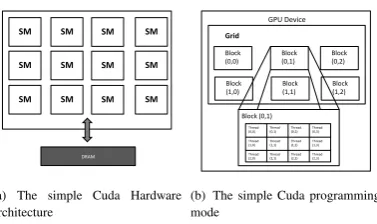
Using GPU as a general computing unit has attracted considerable attention. GPU provides massive parallel processing power. As the host for the GPU device, CPU organizes and invokes the kernel functions that execute on GPU. As shown in Figure 1(a), a GPU device consists of a number of streaming multiprocessors (SM), each comprising simple processing engines, called CUDA cores in the NVIDIA terminology [29]. Each SM has its own shared memory, which is equally accessible by all CUDA cores in the SM. At any given cycle, the CUDA cores in a SM execute the same instruction on different data items. SMs communicate with each other through the global memory of GPU.
DRAM SM
SM
SM SM
SM
SM SM
SM
SM SM
SM
SM
(a) The simple Cuda Hardware architecture
GPU Device
Block (0,0)
Block (1,0)
Block (0,1)
Block (1,1)
Block (0,2)
Block (1,2) Grid
Block (0,1)
Thread (0,0) Thread (0,1) Thread (0,2) Thread (0,3)
Thread (1,0) Thread (1,1) Thread (1,2) Thread (1,3)
Thread (2,0) Thread (2,1) Thread (2,2) Thread (2,3)
(b) The simple Cuda programming mode
Fig. 1 CUDA programming Model
parallel. A warp is a collection of threads that can run simultaneously on a streaming multiprocessor (SM). The warp size is fixed for a specific GPU. The programmer decides the number of blocks and threads to be executed. If the number of threads is more than the warp size, they are time-shared internally on the SM. A collection of threads (called a block) runs on a multiprocessor at a given time. Multiple blocks can be assigned to a single multiprocessor and their execution is time-shared. A single execution generates a number of blocks. A collection of all blocks in a single execution is called a grid (Figure 1(b)). All threads of a block executing on a single multiprocessor divide its resources equally amongst themselves. Each thread and block is given a unique ID that can be accessed within the thread during its execution. Each thread executes a single instruction set called the kernel.
4
Algorithm
for
finding
all
similar
subsequences
In this section, we propose a novel subsequence pattern mining algorithm. The objective of our algorithm is to discover all similar subsequences between two time series. Our proposed algorithm is based on the classical dynamic time warping algorithm and is adapted so that it can capture all subsequence patterns. We first introduce an intuitive strategy to find all similar subsequences. Then we propose two novel pattern mining algorithms.
4.1 Naive Subsequence Matching
The naive approach is to break the time seriesXinto all possible subsequences, and compare them with all the subsequences of Y using the DTW algorithm and select the best matches based on the defined matching condition. That is, for allXs = (xi, xi+1, . . . , xi+k),
where 1 ≤ i ≤ n−k, compute the DTW distance against allYs = (yj, yj+1, . . . , yj+l), where1 ≤ j ≤
m−l,nandmare the length ofXandY respectively. This approach will computemDTW matrix for every timestamp inX, this is because it needs to examine all possibilities. Therefore, the complexity of this method is in quadratic time:O((1 + 2 +· · ·+n)(1 + 2 +· · ·+
m)) =O(n2m2).
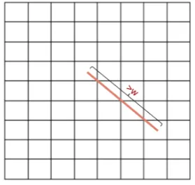
Another brute force method is to use the shotgun window and try to match every possible window between the two sequences. For each window in the first sequence, compute DTW for all windows in the second sequence, and select the pairs with the best match, that is, with the lowest DTW cost. Figure 2 illustrates this approach. The complexity of the shotgun window approach isO(m2n2/w2), which only reduces
the complexity by w2 times. These naive approaches
are not suitable for large-scale datasets, as the time complexity increases quadratically.
Fig. 2 The brute force shotgun windows approach. In these figures, the x-axis represents the length of input time series data (number of data points), the y-axis represents the value of each data point.
Both algorithms presented in this section need to examine all possible combinations between different time series. Hence, the time complexity of both algorithms is high, which motivates us to design more efficient algorithms to find all similar patterns between two time series.
4.2 Proposed algorithm
[image:5.595.74.263.103.215.2] [image:5.595.325.509.345.538.2]data points is large, it is less likely that it will lead to a similar pattern.
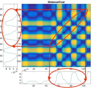
To verify our hypothesis, we conducted the following experiment. For two time series X and Y, we use the cost function to compute the distance between every data point and store the results in a matrix. We call this matrix the cross-distance matrix between two sequences, the value stored in each cell represents the distance between data pointsxi and yj. We visualise
this matrix in Figure 3. In this figure, the darker area represents small values, and they correspond to the data points that have a shorter distance. From Figure 4, we can see that the alignments lie in the low-cost areas in the matrix, where the colours are the darkest in the visualisation.
Fig. 3 Normalised Manhattan Cost Matrix. In two input data frames, the x-axis represents the length of input time series data (number of data points), the y-axis represents the value of each data point. The x and y-axes in the Distance/Cost matrix represent the distance between two corresponding data points.
Fig. 4 Annotated Cost Matrix. In two input data frames, the x-axis represents the length of input time series data (number of data points), the y-axis represents the value of each data point. The x and y-axes in the Distance/Cost matrix represent the distance between two corresponding data points.
Based on the finding above, we modify the classic DTW algorithm so that it will only search for similar subsequences from the low-cost values cells.
In this algorithm, we first determine the low-cost values of the input time series. To achieve this, we introduce the cost thresholdt, which is defined as the minimum average cost for each matching data points. This threshold t is used to determine whether to start or continue a DTW calculation. The procedure should accept the alignment(i, j)(1 ≤i ≤ N and1 ≤j ≤
M) ifdtwDistancedtwLength < t, where:
dtwDistance= X
i,j∈warppingP ath
cost(xi, yj) (5)
anddtwLengthis the length of the warpping path.
If the DTW distance is smaller than this threshold, the path is considered as a possible match and will be included in the further computation.
To avoid over-warping in the warping path during the searching, the window constraint is imposed on the computation. In this method, we define an offset thresholdoto control the length of the warping window, as illustrated in Figure 5. In this figure, the warping window is defined by the red region, and the threshold
o is the length of the warping window offset from the starting position. With the offset threshold, the computation of DTW will stop when the computation reaches the warping window boundary, and therefore, the warping path will not exceed the length of the warping window.
Fig. 5 Offset Threshold and Warping Window
In some cases, the matching subsequences founded by the DTW algorithm may be too short to be considered as a valid match. To tackle this problem, we define the window threshold w to filter out the subsequences that are too short. The window threshold
[image:6.595.89.250.320.452.2] [image:6.595.351.488.516.649.2] [image:6.595.94.248.553.699.2]is a warping path, the length of the warping path must be longer thanwfor the subsequence to be considered.
Fig. 6 Window Threshold: Warping Path Length
4.3 Formal Definition of the algorithm
Based on the discussion in the previous sections, we first summarise the problem as the following:
Given sequence X = (x1, x2, . . . , xn) of length n and sequence Y = (y1, y2, . . . , ym) of length m, the algorithm searches for all subsequence S =
si, si+1, . . . , si+k, where S is a set of all subsequence
of bothXandY that satisfy the following conditions:
(1) The cost of the alignment per data point is less than t, that is, dl <= t. Where : d is total cost of the alignment, i.e. the sum of the cost of every alignment point in the warping path of the matching subsequence; l is the length of the warping path, i.e. the total number of the alignment points in the warping path.
(2) The offset of the warping path from the perfect diagonal line must not exceed o data points, as explained in subsection 4.2.
(3) The length of the warping path must be longer than the window threshold w, as explained in subsection 4.2. If the found match is too short, i.e. smaller thanw, this match will not be included in the final result.
The proposed algorithm is based on the dynamic programming, which updates a matrix of size m×n, wheremandnare the length of two time serialsXand
Y respectively. In our algorithm design, we first create the following matrix to store the intermediate and final results:
• D: This matrix is used to hold the cumulative time warping cost, which takesO(mn)space.
• C: This matrix is used to store the distance between two data points. It is worth noting that this matrix is optional, since the cost between two data points can be computed on the fly while updating
D.
• L: This matrix stores the current length of the warping path of the corresponding alignment. We increment the length of warping path while calculating the cumulated cost and finding the matched subsequences. We use the value stored in this matrix to determine if the match can be included in the final results.
• R: This matrix is the region-marking matrix that stores the position of the start point and end point of the matched subsequences, which will be used in the lookup and the trace-back processes.
• P: This matrix is used to store the direction of previous alignment point of the warping path, which is used in trace back to find the warping path.
The proposed algorithm is performed in three steps: initialisation, update the matrix, and find the path(trace back), which are detailed as follows.
(1) Initialisation: The algorithm initialises all the matrices to zero and initialises cumulative cost matrix D to infinity. Therefore, during the update, the infinity will be ignored in the minimum comparison. If required, the cost matrixCcan be computed.
(2) Subsequence DTW calculation : This step performs the modified DTW algorithm. The algorithm starts from the top left position of the matrices, and iterates these matrices in the diagonal order.
[image:7.595.97.237.139.271.2]If the cell being examined belongs to a warping path, then we select the cell with the smallest cumulative cost from the warping path. Next, we compute the average cost by adding the cost of the current position to the cumulative cost and divide this value by the total length. If the sum of the average cost and the cost of the current cell are smaller than thresholdt, we include this cell as part of the matching subsequence from the cell with the smallest cumulative cost in the warping path, and updateL,D,R,P respectively.
If all the elements in the warping path are not part of any matching subsequences, we first determine if the cost of this cell is smaller thant. If it is, then we start a new subsequence from the current cell and update all the matrices accordingly.
(3) Finding Paths: in this step the algorithm simply uses matrix R and L to find all the matched subsequences. The algorithm also uses threshold
w to check if the length of the warping path is valid, then use P to trace back the warping path and return the results.
We outlined the above procedure in algorithms 1 and 2.
4.3.1 Further improvement
The algorithm described in the last section uses the minimum cumulative cost in matrix D to select the best cell for the DTW path. This approach requires the computation of the cumulative cost and the extra memory to store the results. Therefore, in this section, we propose a greedy algorithm to overcome this problem and further improve the performance.
The design of the greedy algorithm is based on the Markov assumption. That is, instead of using the cumulative cost, we only select the cell with the minimum cost from the warping path, and assume that the path from this cell will lead to a path with the lowest cumulative cost. With this assumption in mind, we change line 10 and line 12 in Algorithm 1 to Equation 6 and 7, respectively, and remove lines 16 and 22.
minpre=min(C[i, j−1], C[i−1, j], C[i−1, j−1]); (6)
mini, minj=argmin([C[i, j−1)], C[i−1, j], C[i−1, j−1]); (7)
However, compared to the original design, the greedy algorithm does not achieve significant improvement in terms of performance and space. This is due
Procedure 1:DTW-based Subsequence Pattern Mining
Input:Time seriesXandY, thresholdtando
Output:Matrices with subsequence matching info:D,L,R,P
1 Initialisation:Dtoinf;
2 L,RandPto 0 ;
3 calculate cost matrixC;
/* begin dynamic programming */
4 fori = 1 : length(X)do
5 forj =1 : length(Y)do
6 ifi== 1andj== 1then
7 minpre= 0;
8 mini=i;minj=j;
9 else
10 minpre= min(D[i-1,j-1],D[i-1,j],D[i,j-1] ) ;
11 minpre= (minpre==inf) ? 0 :minpre;
// set back to 0 if all previous cells are still in init state
12 mini, minj = argmin(D[i-1,j-1],D[i-1,j],D[i,j-1] ) ;
13 end
14 dtwm= (minpre+C[i, j])/(L[mini, minj] + 1);
15 ifdtwm≤tandL[mini, minj] == 0then
/* start a new region */
16 D[i, j] =C[i, j]; // update dtw distance
17 L[i, j] = 1; // update path length
18 R[i, j] = (i, j, i, j); // update start and end cell
19 else ifdtwm≤tthen
/* continue from previous region */
20 (si, sj, li, lj ) = R[mini, minj] ; // find si, ji as the
region start cell
// if current not diverge too much from offset
21 ifabs((i−si)−(j−sj))< othen
22 D[i, j] =minpre+C[i, j]; // update dtw
distance
23 L[i, j] =L[mini, minj] + 1; // update
path length
24 R[i, j] = (si, sj,0,0); // update start cell
25 P[i, j] = (mini, minj); // update path
26 ifi > liandj > ljthen
// update end cell if furthest away
27 R[si, sj] = (si, sj, i, j);
28 end
29 end
30 end
31 end
Procedure 2:Find Paths
Input:Matrices with subsequence matching info:L,R,P, thresholdo Output:Matrices Path marking :OP
1 Initialisation:OPto 0 ;
2 fori = 1 : length(X)do
3 forj =1 : length(Y)do
// if this is the start
4 ifL[i, j] == 1then
5 , , li, lj=R[i, j]; // find end position
6 ifL[li, lj]> wthen // if path length > w
7 whileli > siandlj > sjdo
8 markOP[li, lj]as matching sequence path;
9 (li, lj) =P[li, lj]; // get previous
step
10 end
11 markOP[li, lj]as matching sequence path;
12 end
13 end
14 end
to the following reasons. First, since the original algorithm is based on dynamic programming, in every iteration the cumulative cost is computed based on the result produced in the last step. Therefore, computing the cumulative cost is not an expensive operation. Second, although the greedy algorithm does not require matrix D to store the cumulative cost, it still uses all the rest matrices in computation. Hence, the space complexity is not reduced significantly. In addition, the greedy algorithm cannot find the optimal path because it only uses the local optimal results in finding the subsequence. However, in the DTW algorithm, the local optimal result may not lead to the global optimal solution.
5
GPU Acceleration
In this section, we discuss how to use CUDA to parallelize the algorithm presented in last section. We first introduce the parallelisation strategy used in our design, and then present the CUDA implementation. Further, we present our method to optimise this GPU implementation for the GPU memory hierarchy.
5.1 Data Dependencies
Recall that our algorithm uses the DTW algorithm as core to search for similar patterns. In DTW algorithm, however, the computation of each iteration depends on the result from the last step, which will limit the parallelisation degree during the computation. Therefore, we first analyze the data dependencies in our algorithm and then design a strategy to improve the parallelisation degree.
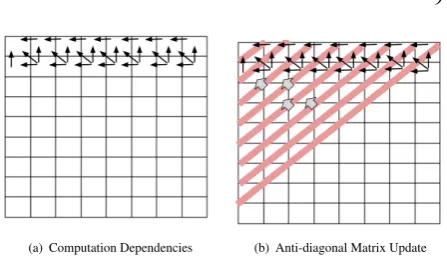
We show the data dependencies of the DTW computation in 7(a). In the matrix, each cell represents the DTW distance between two data points. The computation of each cell depends on the results from left, top, and top-left cells. That is, for cell(i, j)in the matrixD, the value ofD[i, j]depends on the values in
D[i, j−1],D[i−1, j], andD[i−1, j−1].
Therefore, for any cell (i, j) in the matrix, all cells between (0,0)and (i, j) need to be computed before calculating the value of position (i, j). In the classic DTW algorithm, this computation is carried out in the row or column order. The cells in the same row or column are computed in sequence. On the other hand, there is no data dependency between the diagonal cells, as illustrated in 7(b). The cells connected by a red stripe have no data dependency. Therefore, these cells can be computed in parallel. The data dependency exist
(a) Computation Dependencies (b) Anti-diagonal Matrix Update
Fig. 7 Matrix Update Order
between two neighbouring red strips. Therefore, we can only compute the data within one red strip at time. We illustrate this in 7(b) with grey arrow. The arrow indicates the data dependency and compute direction.
Based on the above discussion, we can summarise the parallel strategy as follows. The computation starts with the first cell, then updates the cells in the closest diagonal lines (the red stripe in 7(b)). Since these cells only depend on the first cell, they can be computed in parallel. Then the computation moves to the next diagonal line. By updating the matrix in this way, it is guaranteed that the data dependency is not broken and the reasonable degree of parallelism can be achieved.
5.2 Implementation of Parallelisation strategy
The previous section outlines a strategy to update the matrix in diagonal order. In this section, we describe how to implement this strategy in CUDA.
To implement this strategy on GPU, we need to consider how to map the CUDA threads to the data that need to be processed. Recall that the parallel diagonal computation model solves the data dependency issue by computing the matrix cells in diagonal order. Therefore, for each diagonal line, we can assign one thread to a cell within this line, and compute these cells in parallel.
An intuitive method to implement this strategy is to launch one kernel with enough threads, the number of threads within this kernel is larger or equal to the longest diagonal. In this design, the computation forms a loop within the kernel and each iteration processes one diagonal line. By implementing the algorithm in this way, we only need to launch one kernel, and therefore, reduce the overhead of multiple kernel launch.
[image:9.595.310.534.86.215.2]…… threads:
t1 t2
t3 t4
t5
nx
ny
ny-1
synchronise
synchronise synchronise synchronise synchronise
synchronise synchronise synchronise synchronise
synchronise synchronise synchronise
synchronise
synchronise synchronise
Fig. 8 Subsequence DTW Matrix Update Threading
the first one starts the processing when the previous thread finishes processing one cell in the matrix. By arranging the computation in this way, we can ensure that the data dependency is preserved and the data in the same diagonal line can be processed in parallel. This is because when the first thread processes the first cell in the matrix, the rest threads are waiting for this thread to finish. Once this computation is finished, the thread moves to the next item in the column, and its consecutive thread can start processing the first cell in the column assigned to it. These two threads can run in parallel because the cells involved in the computation can form a diagonal line in the matrix, and therefore, there are no dependency between them. However, as we mentioned in the last section, the results of the cells within a diagonal line depend on the cells in the previous diagonal line. Therefore, to enforce this dependency, we need to synchronise all threads involved in the computation along the diagonal line. We illustrate this design in Figure 8. In this Figure, the orange area represents the matrix that needs to be processed, the threads are represented by the red arrow, and the synchronisation point is labelled by the red diagonal line.
From this Figure, we can see that the computation
forms a parallelogram. The number of threads needed in the computation equals to the height of this parallelogram, which is ny. And the number of iterations required equals to the base of the parallelogram, which isnx+ny−1number of rows. Therefore, the time complexity of this implementation is: O(nx+ny−1), which is a significant reduction fromO(nx×ny).
5.3 Memory Access Optimisation
Coalesced access data in the global memory is critical to the performance of a GPU application. Non-coalesced memory access will lead to poor performance. In this section, we present how to enforce the coalesced memory access by enabling the consecutive threads to access consecutive memory address in our implementation.
Recall that our initial implementation processes the data in the diagonal order. However, the data is stored as a matrix in the memory, and the elements on one diagonal line are not stored consecutively in the memory. Therefore, to achieve the coalesced access to the global memory, the data stored in the memory need to be rearranged so that the elements on the same diagonal line are stored consecutively in the GPU memory.
Intuitively, rearranging the matrix can be achieved by reallocating another 2D array. In this new array, the length ofx-dimension is the length of the longest diagonal line in the original matrix, while the y -dimension is the number of the diagonal lines in the original matrix. In the new array, the diagonal lines from the original matrix are stored consecutively in the memory. We illustrate the array in Figure 9.
0,0 0,1 0,2 0,3 0,4 0,5 0,6 1,1 1,2 1,3 1,4 1,5 1,6 1,7 2,1 2,2 2,3 2,4 2,5 2,6 2,7 3,1 3,2 3,3 3,4 3,5 3,6 3,7 4,1 4,2 4,3 4,4 4,5 4,6 4,7 5,1 5,2 5,3 5,4 5,5 5,6 5,7 6,1 6,2 6,3 6,4 6,5 6,6 6,7 7,1 7,2 7,3 7,4 7,5 7,6 7,7 8,1 8,2 8,3 8,4 8,5 8,6 8,7
(a) Original Matrix
0,0
1,1 0,1
2,1 1,2 0,2
3,1 2,2 1,3 0,3
4,1 3,2 2,3 1,4 0,4
5,1 4,2 3,3 2,4 1,5 0,5
6,1 5,2 4,3 3,4 2,5 1,6 0,6
7,1 6,2 5,3 4,4 3,5 2,6 1,7
8,1 7,2 6,3 5,4 4,5 3,6 2,7
8,2 7,3 6,4 5,5 4,6 3,7
8,3 7,4 6,5 5,6 4,7
8,4 7,5 6,6 5,7
8,5 7,6 6,7
8,6 7,7
8,7
(b) Diagonal Matrix
[image:10.595.86.236.104.392.2] [image:10.595.321.522.583.740.2]However, as shown in the Figure, storing the diagonal line into the new matrix leads to the waste of memory space. To address this problem, instead of storing the diagonal line into a 2D array, we use a flat array to store the data from the diagonal line consecutively.
In addition, when calculating the warping boundary for the offset threshold, it is necessary to know the row and column position of each element. Therefore, we create another matrix, namely index matrixI, to store the index of the flat array in the corresponding row and column position.
The array indices can be determined through mathematical derivation, and be calculated in the initialisation step in parallel. In the next section, we present how to derive these index numbers in the matrix.
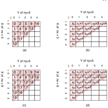
5.3.1 Calculating diagonal index
We draw some small matrix and fill in the index number to study the relationship between the array index and the row and column(i, j)in the matrix. The indices in the upper left corner and bottom-right corner in the matrix should be calculated differently. This is due to the following reason. If the index is computed from left to right, then the upper left part starts from the left most column, while the bottom right part starts from the bottom most row. As shown in the Figure 10 and Figure 11, these figures outlined two situations of the index number. The matrix represents the alignment of sequenceXandY, where the size ofXisnxand size
ofY isny. The matrix size isnx×ny; the row index is
represented byiwhile the column index is represented by j, as shown in the figure. The red arrows in the matrix represents the direction of the increment of the array index.
Top-left:
As illustrated in Figure 10, whenj < nx−i, the array
index falls into the top left part in the matrix. We denote the index of an element in the left most column asSi,
where iis the row index of the element. As shown in Figure 10(b), the number increases along the red arrow from the left most column. E.g.index(0,1) =S1+ 1;
index(1,3) =S4+ 3.
For an arbitrary element residing in the top left part of the matrix (i.e. j < nx−i), if we denote the start
position of the diagonal line that this element belongs to as Sistart, then we can compute its index by the
following formula:
[image:11.595.307.535.87.316.2]index(i, j) =Sistart+j (8)
Fig. 10 Optimised memory access index - top left
Because for any arbitrary element it forms a right triangle withxandy-axes, the position ofistartcan be
found by counting the number of steps needed for this arbitrary element to reach the leftmost column:
istart=i+j (9)
Since the number of elements in each diagonal line increases in each line, we can use the arithmetic sequence to calculate theSistart. However, as illustrated
in Figure 10(c) and (d), whennx> ny, the computation
has to be considered carefully. Since when the length of
x-axis is greater than that of the y-axis, the arithmetic sequence stops atny and increases byny in each row,
which can be formally defined as:
istart> ny
⇒i+j > ny (10)
Hence, we separate the computation in following two cases:
• Case:i+j < ny
Recall that the sum of an arithmetic sequence can be calculated by:
Sn =
n(a1+an)
2
where:
Sn :sum ofnterms;
a1:first term;
As illustrated in Figure 10(a) and (b) we get:
Sistart= 0 + 1 + 2 +· · ·+istart
= istart×(istart+ 1) 2
(11)
Substituting Equation 11 with Equation 8 and Equation 9:
index(i, j) =Sistart+j
= (i+j)×(i+j+ 1)
2 +j
• Case:i+j≥ny
As illustrated in Figure 10(c) and (d), we get:
Sistart = 0 + 1 + 2 +· · ·+ (ny−1) + (istart−ny+ 1)×ny
=(ny−1)×ny
2 + (istart−ny+ 1)×ny
(12)
Substituting Equation 12 with Equation 8 and Equation 9:
index(i, j) =Sistart+j
=(ny−1)×ny
2 +
(i+j−ny+ 1)×ny+j
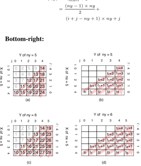
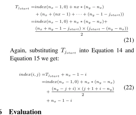
[image:12.595.54.280.372.637.2]Bottom-right:
Fig. 11 Optimised memory access index - bottom right
We now considering the case when j ≥ nx −i,
i.e when the position falls into the bottom-right part of the matrix as shown in Figure 11. Similar to the top-left case, two cases need to be considered, as shown in Figure 11(a),(b) and (c),(d).
We denote the cells (i, j) in the bottommost row (i.e, where the red arrows start from) as Tjstart. The
index(i, j) equals to Tjstart adding the row index
counting from the bottom (called the reverse row index). We denote the reverse row index by i0, which can be computed by the formula:
i0=nx−1−i (13)
Hence, we can calculate theindex(i, j)by:
index(i, j) =Tjstart+i0
=Tjstart+nx−1−i
(14)
Similar to the Top-left case, thejstartis the number
of steps required to reach the left most column from the current row:
jstart=j−i0
=j−nx+ 1 +i
(15)
The arithmetic sequence is used to calculate the
Tjstart. In this case, the sequence is in the decreasing
order fromnytony−1−jstart. Hence, the arithmetic
sequence starts at the point when:
jstart> ny−nx
⇒j−nx+ 1 +i > ny−nx (16)
When ny > nx, the computation needs to be
addressed differently. Hence, we handle the calculation in following 3 cases:
• Case:ny≤nx
Tjstart=index(nx−1,0) + (ny+ (ny−1)
+· · ·+ (ny−1−jstart))
=index(nx−1,0)+
(ny+ny−1−jstart)×(jstart)
2
(17)
Substituting Equation 14 and Equation 15:
index(i, j) =index(nx−1,0)+
(2ny−j+nx−i)×(j−nx+ 1 +i)
2 +nx−1−i
(18)
• Case:ny> nxandjstart ≤ny−nx
In this case, theTjstart is defined as:
Tjstart=index(nx−1,0) +nx×jstart (19)
By substituting Equation 14 and Equation 15, we can compute theindex(i, j)as:
index(i, j) =Tjstart+nx−1−i
=index(nx−1,0)+
nx×(j−nx+ 1 +i) +nx−1−i
(20)
• Case:ny > nxandjstart> ny−nxIn this case,
Tjstart=index(nx−1,0) +nx∗(ny−nx)
+ (nx+ (nx−1) +· · ·+ (ny−1−jstart))
=index(nx−1,0) +nx∗(ny−nx)+
(nx+ny−1−jstart)×(jstart−(ny−nx))
2
(21)
Again, substituting Tjstart into Equation 14 and
Equation 15 we get:
index(i, j) =Tjstart+nx−1−i
=index(nx−1,0) +nx∗(ny−nx)
+(ny−j+i)×(j+ 1 +i−ny) 2
+nx−1−i
(22)
6
Evaluation
To evaluate the effectiveness and efficiency of the proposed pattern mining algorithm, we have conducted extensive experiments with different time series dataset drawn from real life. We first apply the proposed algorithm on different datasets to evaluate the ability of the proposed pattern mining method in capturing the repeated patterns between two time series. Then we evaluate the performance of the serial implementation and the parallel implementation. Finally, we evaluate our proposed technique for memory optimisation.
6.1 Preprocessing and parameters setting
We first evaluate the effectiveness of our proposed algorithm. In our experiments, the data preprocessing is needed before the pattern mining process. The preprocessing step includes removing trend, using Haar-wavelet-transfrom to smooth and reduce the complexity of time series with much noise and fluctuation. Preprocessing is beneficial to pattern mining, for example, the preprocessing steps such as Haar-wavelet-transform can reduce the size of the data, and hence will reduce the computation time.
In our experiments, we use the normalised cost threshold, offset threshold and window threshold. Hence, the same parameters can be applied on different datasets. In normalised cost threshold, we use the normalised cost function described in subsection 3.3. Therefore, the cost are in the range between 0 to 1. The time-series data should also be normalised in the preprocessing step if they are in similar ranges. In normalised offset and window threshold, we represent the offset/window as a factor of the average length of the time series instead of actual size. Therefore, the threshold parameters are independent on the dataset.
6.2 Subsequence Pattern Mining
A number of experiments have been conducted to evaluate the quality of proposed DTW-based pattern mining algorithm. In this section, we evaluate the algorithm with different datasets. The dataset used in these experiments are from the real world, synthetic data and random data.
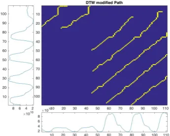
6.2.1 Experiments with internet traffic data
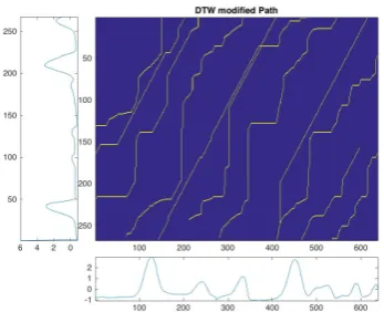
[image:13.595.55.288.106.302.2]Our first experiment is conducted by applying our algorithm on the datasets containing the same subsequence with different order. In this experiment, we use a subset of internet traffic data from The Time Series Data Library (TSDL) [30]. We crop a small piece of sequence, around 100 data points, as test datasetX. We also select another set of data with the similar length from the original dataset as datasetY, and certain data in datasetsXandY are overlapped. In this experiment, we set the thresholds to the following values: t = 0.13, o = 0.15, w = 0.2. The DTW cumulative cost matrix and paths for discovered subsequences are visualised in Figure 12 and Figure 13, respectively.
Fig. 12 Modified DTW method cumulative cost matrix. In two input data frames, the x-axis represents the length of input time series data (number of data points), the y-axis represents the value of each data point. The x and y-axes in the Distance/Cost matrix represent the distance between two corresponding data points.
[image:13.595.334.511.413.552.2]Fig. 13 Modified DTW method matched subsequence paths. In two input data frames, the x-axis represents the length of input time series data (number of data points), the y-axis represents the value of each data point. The x and y-axes in the matrix represent the distance between two corresponding data points.The matching subsequences between two data frames are shown with the yellow line.
to capture the subsequence pattens between the time series. The exact subsequence is discovered, along with other similar subsequences.
This experiment shows that the modified DTW method picks up the local alignment regions in the matrix first, then calculates the possible subsequence alignments path. However, executing the algorithm with different distance function and thresholds will generate slightly different alignment results. Although the algorithm will find different alignments, these alignments will still correspond to the similar subsequence between two sequences.
6.2.2 Effect of different thresholds
The thresholds designed in the proposed algorithm can help the algorithm to discover the patterns and have impact on subsequence found by the algorithm. In this section, we study how the threshold values will affect the performance of proposed algorithm.
In these experiments, we use the same dataset from the previous section. This way, we can see the effect on the results with different thresholds. We first study the cost thresholdt, which controls the toleration of the matching subsequence. In this experiment, we reduce the thresholdtfrom 0.13 to 0.05. The results are shown in Figure 14.
The results shows that by reducing the cost threshold, the subsequences found by the algorithm lie in the lower cumulative cost in the path. Therefore, these subsequences are more similar. On the other hand,
Fig. 14 Result with lower cost threshold. In two input data frames, the x-axis represents the length of input time series data (number of data points), the y-axis represents the value of each data point. The x and y-axes in the matrix represent the distance between two corresponding data points.The matching subsequences between two data frames are shown with the yellow line.
with larger value t, the algorithm will produce more matching sequences as it will consider more candidates. We then study the effect of threshold o. This threshold controls how much the path can be diverged from the perfect matching sequence path (i.e a one to one correspondence in time warping path). If the offset thresholdois too big, the discovered path will include long tails as demonstrated in Figure 15, which uses a larger offset threshold of 1. On the other hand, if the offset is too small, the result may only include the straight path and they may be clustered together. Unlike other thresholds, the offset threshold o has a bigger influence on the quality of the result.
The window threshold is used to filter out the shorter sequences and only report the matching sequences that have the warping path longer than the threshold. In this experiment, we increase the window threshold from 0.2 to 0.3 and plot the results in Figure 16. From this figure, we can see that by increasing the window length, the results produced by the algorithm is less than the small threshold.
6.2.3 Experiments with the data containing spikes - WordsSynonyms
[image:14.595.338.511.107.245.2]Fig. 15 Result with large offset threshold. In two input data frames, the x-axis represents the length of input time series data (number of data points), the y-axis represents the value of each data point. The x and y-axes in the matrix represent the distance between two corresponding data points.The matching subsequences between two data frames are shown with the yellow line.
Fig. 16 Result with larger window threshold. In two input data frames, the x-axis represents the length of input time series data (number of data points), the y-axis represents the value of each data point. The x and y-axes in the matrix represent the distance between two corresponding data points.The matching subsequences between two data frames are shown with the yellow line.
data from UCR Time Series Classification Archive [31], which contains the possible patterns but also contains the spikes in one of the sequences. In this dataset, the training and testing datasets are different but are from the same source.
We compare the training and testing data from this dataset to evaluate our pattern mining algorithm. Unlike the training data, the testing dataset contains spikes in it. In order to see how well our algorithm performs, we compare the results produced with the original dataset against the dataset with the spikes
being removed. There are many different techniques to remove the spikes from the dataset. In our experiment, we choose Median filter to eliminate the spikes in time series dataset due to the popularity of this methods. The experiment results are shown in Figure 17 and Figure 18.
Fig. 17 Result of WordsSynonyms data. In two input data frames, the x-axis represents the length of input time series data (number of data points), the y-axis represents the value of each data point. The x and y-axes in the matrix represent the distance between two corresponding data points.The matching subsequences between two data frames are shown with the yellow line.
Fig. 18 Result of WordsSynonyms data filtered. In two input data frames, the x-axis represents the length of input time series data (number of data points), the y-axis represents the value of each data point. The x and y-axes in the matrix represent the distance between two corresponding data points.The matching subsequences between two data frames are shown with the yellow line.
[image:15.595.337.511.466.607.2]is resistant to spikes in the data and it will treat them as part of the pattern.
6.2.4 Experiments with the circular trend data
[image:16.595.333.512.103.245.2]In this section we evaluate the performance of proposed algorithm with the data that have the circular patterns. In this experiment, we use the data with the repeating patterns and the increasing trend (the absolute value of the data increases over time) from TSDL [30]. The time series is tested against itself in this experiment to see how our method handles the type of time series data. We create another dataset by removing the trend in the data, and compare the results with the original dataset. As we can see from Figure 19 and Figure 20, our algorithm is able to is able to pick up all the circular patterns after removing the trend.
Fig. 19 Data with circular trend. In two input data frames, the x-axis represents the length of input time series data (number of data points), the y-axis represents the value of each data point. The x and y-axes in the matrix represent the distance between two corresponding data points.The matching subsequences between two data frames are shown with the yellow line.
6.2.5 Experiments with noisy data - cluster load
We then evaluate our algorithm using the data with the noisy signals. In this experiment, we use two sets of trace data in clusters from [32]. The result alignments look very scattered without any preprocessing. To improve the result, we applied the Haar Wavelet transform [33] to the data sequence. Figure 21 and Figure 23 show the result before and after applying the Haar-Wavelet-transform to the two sets of data. Figure 22 and Figure 24 demonstrate that the paths of the patterns in the cost matrix. The results show that the patterns are discovered correctly.
6.3 Performance
[image:16.595.79.257.323.463.2]In this section, we conduct the performance analysis on both serial and parallel implementation. In these
Fig. 20 Data with circular trend - removed trend. In two input data frames, the x-axis represents the length of input time series data (number of data points), the y-axis represents the value of each data point. The x and y-axes in the matrix represent the distance between two corresponding data points.The matching subsequences between two data frames are shown with the yellow line.
Fig. 21 Haar wavelet transform on complicated time series. In these figures, the x-axis represents the length of input time series data (number of data points), the y-axis represents the value of each data point.
experiments, we use a very large dataset collected by [34]. We test the performance by using different implementations to analyze a subset of the data with different lengths. The experiments are conducted on a machine with NVIDIA Tesla K40 GPU with 12GB memory. We use a subset from the dataset that can fit into the GPU memory.
6.3.1 Serial vs CUDA Implementation
[image:16.595.326.533.358.520.2]Fig. 22 Modified DTW on transformed sequence. In two input data frames, the x-axis represents the length of input time series data (number of data points), the y-axis represents the value of each data point. The x and y-axes in the matrix represent the distance between two corresponding data points.The matching subsequences between two data frames are shown with the yellow line.
Fig. 23 Haar wavelet transform on complicated time series. In these figures, the x-axis represents the length of input time series data (number of data points), the y-axis represents the value of each data point.
serial implementation (Host Matrix) and the CUDA implementation (CUDA Matrix).
From the figure, we can see that the CUDA implementation achieves the faster execution time than the serial implementation.
We then compare the execution time between the CUDA implementation and the CUDA implementation with the optimised memory access.
[image:17.595.347.504.106.238.2]It can be seen from Figure 26 that by optimising the memory access the optimised CUDA implementation has the shorter execution time. This result demonstrates the effectiveness of our technique in optimising the memory access.
Fig. 24 Modified DTW on transformed sequence. In two input data frames, the x-axis represents the length of input time series data (number of data points), the y-axis represents the value of each data point. The x and y-axes in the matrix represent the distance between two corresponding data points.The matching subsequences between two data frames are shown with the yellow line.
Fig. 25 Execution time of the serial and CUDA
implementations. The x-axis represents the length of input
time series data (number of data points), the y-axis represents the execution time in millisecond.
Fig. 26 Comparison of dtwm calculation time. The x-axis represents the length of input time series data (number of data points), the y-axis represents the execution time in millisecond.
7
Conclusion
[image:17.595.325.517.342.481.2] [image:17.595.76.279.353.514.2] [image:17.595.322.518.540.667.2]algorithm first identifies the possible start positions of similar alignments, and then uses the dynamic programming technique to expand the subsequences. Further, we parallelize the proposed algorithm using GPGPU and CUDA, and develop a optimization technique to improve the memory access in the GPU implementation. Extensive evaluation experiments have been conducted. The results show that our algorithm can discover similar subsequences between two time series and achieve much better performance with the GPU parallelisation.
Acknowledgment
This research is supported by the Natural Science Foundation of China NO.61602215, the science foundation of Jiangsu province NO.BK20150527, the EU Horizon 2020Marie Sklodowska-Curie Actions through the project entitled Computer Vision Enabled Multimedia Forensics and People Identification (Project No. 690907, Acronym: IDENTITY).
References
[1] Philippe Esling and Carlos Agon. Time-series data mining.ACM Computing Surveys (CSUR), 45(1):12, 2012.
[2] Chang-Tsun Li, Yinyin Yuan, and Roland Wilson. An unsupervised conditional random fields approach for clustering gene expression time series.Bioinformatics, 24(21):2467–2473, 2008.
[3] Kin-Pong Chan and AW-C Fu. Efficient time series matching by wavelets. InData Engineering, 1999. Proceedings., 15th International Conference on, pages 126–133. IEEE, 1999.
[4] Xianping Ge and Padhraic Smyth. Deformable markov model templates for time-series pattern matching. InProceedings of the sixth ACM SIGKDD international conference on Knowledge discovery
and data mining, pages 81–90. ACM, 2000.
[5] Konstantinos Kalpakis, Dhiral Gada, and Vasundhara Puttagunta. Distance measures for effective clustering of arima time-series. In Data Mining, 2001. ICDM 2001, Proceedings IEEE International
Conference on, pages 273–280. IEEE, 2001.
[6] Jessica Lin Eamonn Keogh Stefano Lonardi and Pranav Patel. Finding motifs in time series. In
Proc. of the 2nd Workshop on Temporal Data Mining,
pages 53–68, 2002.
[7] Bill Chiu, Eamonn Keogh, and Stefano Lonardi. Probabilistic discovery of time series motifs.
In Proceedings of the ninth ACM SIGKDD
international conference on Knowledge discovery
and data mining, pages 493–498. ACM, 2003.
[8] Gautam Das, King-Ip Lin, Heikki Mannila, Gopal Renganathan, and Padhraic Smyth. Rule discovery from time series. InKDD, volume 98, pages 16–22, 1998.
[9] Frank Hppner. Discovery of temporal patterns. In Luc De Raedt and Arno Siebes, editors, Principles
of Data Mining and Knowledge Discovery, volume
2168 of Lecture Notes in Computer Science, pages 192–203. Springer Berlin Heidelberg, 2001.
[10] Eamonn J Keogh and Michael J Pazzani. An enhanced representation of time series which allows fast and accurate classification, clustering and relevance feedback. InKDD, volume 98, pages 239– 243, 1998.
[11] Markus Hegland, William Clarke, and Margaret Kahn. Mining the macho dataset. Computer Physics
Communications, 142(1):22–28, 2001.
[12] Dipankar Dasgupta and Stephanie Forrest. Novelty detection in time series data using ideas from immunology. In Proceedings of the international
conference on intelligent systems, pages 82–87,
1996.
[13] Jiawei Han, Guozhu Dong, and Yiwen Yin. Efficient mining of partial periodic patterns in time series database. InData Engineering, 1999. Proceedings.,
15th International Conference on, pages 106–115.
IEEE, 1999.
[14] Meinard M¨uller.Information retrieval for music and motion, volume 2. Springer, 2007.
[15] Christos Faloutsos, M. Ranganathan, and Yannis Manolopoulos. Fast subsequence matching in time-series databases. SIGMOD Rec., 23(2):419–429, May 1994.
[16] Yasushi Sakurai, Christos Faloutsos, and Masashi Yamamuro. Stream monitoring under the time warping distance. In2007 IEEE 23rd International
Conference on Data Engineering, pages 1046–1055.
IEEE, 2007.
Westover, Qiang Zhu, Jesin Zakaria, and Eamonn Keogh. Searching and mining trillions of time series subsequences under dynamic time warping. In
Proceedings of the 18th ACM SIGKDD international conference on Knowledge discovery and data
mining, pages 262–270. ACM, 2012.
[18] X. Wei, C. T. Li, Z. Lei, D. Yi, and S. Z. Li. Dynamic image-to-class warping for occluded face recognition. IEEE Transactions on Information
Forensics and Security, 9(12):2035–2050, Dec 2014.
[19] Machiko Toyoda and Yasushi Sakurai. Discovery of cross-similarity in data streams. In2010 IEEE 26th International Conference on Data Engineering
(ICDE 2010), pages 101–104. IEEE, 2010.
[20] Takuma Nishii, Tomoyuki Hiroyasu, Masato Yoshimi, Mitsunori Miki, and Hisatake Yokouchi. Similar subsequence retrieval from two time series data using homology search. In Systems Man and Cybernetics (SMC), 2010 IEEE International
Conference on, pages 1062–1067. IEEE, 2010.
[21] L. Xiao, Y. Zheng, W. Tang, G. Yao, and L. Ruan. Parallelizing dynamic time warping algorithm using prefix computations on gpu. In
2013 IEEE 10th International Conference on High Performance Computing and Communications 2013 IEEE International Conference on Embedded and
Ubiquitous Computing, pages 294–299, Nov 2013.
[22] Doruk Sart, Abdullah Mueen, Walid Najjar, Eamonn Keogh, and Vit Niennattrakul. Accelerating dynamic time warping subsequence search with gpus and fpgas. In 2010 IEEE International Conference on
Data Mining, pages 1001–1006. IEEE, 2010.
[23] Y. Zhang, K. Adl, and J. Glass. Fast spoken query detection using lower-bound dynamic time warping on graphical processing units. In 2012 IEEE International Conference on Acoustics, Speech
and Signal Processing (ICASSP), pages 5173–5176,
March 2012.
[24] Alireza Vahdatpour, Navid Amini, and Majid Sarrafzadeh. Toward unsupervised activity discovery using multi-dimensional motif detection in time series. InIJCAI, volume 9, pages 1261–1266, 2009.
[25] Abdullah Mueen, Eamonn J Keogh, Qiang Zhu, Sydney Cash, and M Brandon Westover. Exact discovery of time series motifs. InSDM, pages 473– 484. SIAM, 2009.
[26] Machiko Toyoda, Yasushi Sakurai, and Yoshiharu Ishikawa. Pattern discovery in data streams under the time warping distance. The VLDB Journal, 22(3):295–318, 2013.
[27] S. Srikanthan, A. Kumar, and R. Gupta. Implementing the dynamic time warping algorithm in multithreaded environments for real time and unsupervised pattern discovery. In 2011 2nd International Conference on Computer and
Communication Technology (ICCCT-2011), pages
394–398, Sept 2011.
[28] N. Takahashi, T. Yoshihisa, Y. Sakurai, and M. Kanazawa. A parallelized data stream processing system using dynamic time warping distance.
In 2009 International Conference on Complex,
Intelligent and Software Intensive Systems, pages
1100–1105, March 2009.
[29] Nvidia Corporation. Nvidia CUDA C ProgrammingGuide, 2011.
[30] R J Hyndman. Time series data library, Accessed on 09/2016.
[31] Yanping Chen, Eamonn Keogh, Bing Hu, Nurjahan Begum, Anthony Bagnall, Abdullah Mueen, and Gustavo Batista. The ucr time series classification archive, July 2015. www.cs.
ucr.edu/˜eamonn/time_series_data/.
[32] Google cluster traces, Accessed on 09/2016.
[33] Radomir S. Stankovic and Bogdan J. Falkowski. The haar wavelet transform: its status and achievements.
Computers and Electrical Engineering, 29(1):25–44,
2003.
[34] Thanawin Rakthanmanon, Bilson Campana, Abdullah Mueen, Gustavo Batista, Brandon Westover, Qiang Zhu, Jesin Zakaria, and Eamonn Keogh. Searching and mining trillions of time series subsequences under dynamic time warping. In
Proceedings of the 18th ACM SIGKDD international conference on Knowledge discovery and data
Huanzhou Zhu received the Bachelors degree in Information System Engineering from Imperial College London, UK, in 2008, and received the Masters and the PhD degree in Computer Science from the University of Warwick, UK, in 2009 and
2016 respectively. He is now a
Post-doctoral researcher at the Imperial College London. His areas of interest are Big data processing systems, parallel and distributed computation systems, high performance Computing, Cloud computing and Computer security.
Zhuoer Gu acquired his BSc at Shanxi University in 2013, and in 2018 he finished his PhD in the University of Warwick. He has focused on time series data mining for
years. His research interests cover time
series analysis and data mining, machine learning and high performance computing.
Haiming Zhaoreceived the B.Eng. degree in Computing from Imperial College
London and M.Sc. degree in Data
Analytics from University of Warwick,
in 2015 and 2016, respectively. Since
then, she has been working as a software engineer in the finance industry.
Keyang Chengis a member of CCF. He received the PHD Degree from School of Computer Science and Engineering, Nanjing University of Aeronautics & Astronautics in 2015. He has co-authored more than 30 journal and conference papers. He was at University of Warwick, UK, as a post-doctoral researcher in 2016. He is currently an assistant professor and researcher in the School of Computer Science and Telecommunications Engineering of Jiangsu University. His current research interests lie in the areas of pattern recognition, computational intelligence and computer vision.
Chang-Tsun Lireceived the MSc degree
in computer science from U.S.Naval
Postgraduate School, USA, in 1992, and the Ph.D. degree in computer science from the University of Warwick, UK, in 1998. He was an associate professor of the Department of Electrical Engineering at NDU during 1998-2002 and a visiting professor of the Department of Computer Science at U.S. Naval
Postgraduate School in the second half of 2001. He was
a professor of the Department of Computer Science at the University of Warwick, UK, until Dec 2016. He is currently a professor of the School of Computing and Mathematics, Charles Sturt University, Australia, leading the Data Science Research
Unit. His research interests include multimedia forensics
and security, biometrics, data mining, machine learning, data analytics, computer vision, image processing, pattern recognition, bioinformatics, and content-based image retrieval. The outcomes of his multimedia forensics and machine learning research have been translated into award-winning commercial products protected by a series of international patents and have been used by a number of police forces and courts of law around the world. He is currently Associate Editor of the EURASIP Journal of Image and Video Processing (JIVP) and Associate Editor of IET Biometrics. He involved in the organisation of many international conferences and workshops and also served as member of the international program committees for several
international conferences. He is also actively contributing
keynote speeches and talks at various international events.
Ligang He received the Bachelors and
Masters degrees from the Huazhong