A randomized neural network for data streams

A Randomized Neural Network for Data Streams

Mahardhika Pratama1)_{, Plamen P. Angelov}2)_{, Jie Lu}3)_{, Edwin Lughofer}4)_{, Manjeevan Seera}5)_{, C. P. Lim}6) 1) School of Engineering and Mathematical Sciences, La Trobe University, Melbourne, Australia, email: [email protected]

2) School of Computing and Communication, Lancaster University, Lancaster, UK, email: [email protected]

3) Center for Quantum Computation and Intelligent Systems, University of Technology Sydney, Sydney, Australia, email: [email protected]

4) Department of knowledge-based mathematical system, Johannes Kepler University, Linz, Austria, email: [email protected]

5)Faculty of Engineering, Computing and Science, Swinburne University of Technology (Sarawak Campus), Malaysia email: [email protected]

6) Institute of Intelligent System Research and Innovation, Deakin University, Geelong, Australia, email: [email protected]

Abstract— Randomized neural network (RNN) is a highly feasible solution in the era of big data because it offers a simple and fast working principle in processing dynamic and evolving data streams. This paper proposes a novel RNN, namely recurrent type-2 random vector functional link network (RT2McRVFLN), which provides a highly scalable solution for data streams in a strictly online and integrated framework. It is built upon the psychologically inspired concept of metacognitive learning, which covers three basic components of human learning: what-to-learn, how-to-learn, and when-to-learn. The what-to-learn selects important samples on the fly with the use of online active learning scenario, which renders our algorithm an online semi-supervised algorithm. The how-to-learn process combines an open structure of evolving concept and a randomized learning algorithm of random vector functional link network (RVFLN). The efficacy of the RT2McRVFLN has been numerically validated through two real-world case studies and comparisons with its counterparts, which arrive at a conclusive finding that our algorithm delivers a tradeoff between accuracy and simplicity.

Keywords—Evolving Fuzzy Systems, Fuzzy Neural Networks, Type-2 Fuzzy Systems, Sequential Learning.

I. INTRODUCTION

Randomized Neural Networks (RNNs) today have regained its popularity because its simple but theoretically sound working principle offers a fast solution to process big data [1]. Random vector functional link network (RVFLN) is among the most prominent RNNs in the literature whose universal approximation capability has been theoretically proven [2]. This in-depth study provides a solid basis for randomly generating all network parameters but the output weight vector. It has concluded the universal approximation property of the RVFLN for any continuous functions on bounded finite-dimensional sets with the rate of approximation error

convergence at

O

(

C

)

n

, where n is the number of basis

functions and C is independent of n [3]. Random learning scenario of neural network significantly simplifies the design process of the neural network and avoids the laborious iterative tuning process.

RNN has transformed into one of the most active research areas in the machine learning community. A randomized learning algorithm for a sparse neural network is put forward in [4]. [5] combines the concept of RNN and the probabilistic learning theory. A local learning algorithm for RNN was put into perspective in [6]. An ensemble learning of RNN is proposed in [7], while [8] concerns the distributed learning scenario of the RNN. RNN has been deployed to various real-world cases: [9] makes use of RNN for short term electricity load forecasting; [10] adopts RNN for face recognition; [11] uses RNN to perform a tool condition monitoring. These works are however an offline learning algorithm, which cannot deal with data streams because it follows a one-shot learning scheme using the pseudo-inversion technique.

RNN has been extended to cope with the online learning situation. [12] offers an incremental parameter learning scenario of RNN which addresses both chunk-by-chunk data stream and one-by-one data stream. This work suffers from the absence of structural learning scenario since it relies on a predetermined network architecture. The concept of a dynamic structure has been introduced in [13] but still works in the batched learning scenario. Furthermore, the rule growing process does not study real data distributions, thereby being unable to handle concept changes in data streams [35]. [14] proposed the drift detection mechanism along with an ensemble of RNN which expands its size when a drift is signaled. In [15], a psychologically inspired metacognitive learning is incorporated for the RNN. Although various extensions of RNN have been studied in the literature, RNN still leaves four open research issues: uncertainty, temporal

system dynamic, concept drift, and curse of dimensionality.

This paper presents a novel RVFLN, namely recurrent type-2 metacognitive random vector functional link network

(RT2RVFLN). The RT2RVFLN implements a

psychologically-inspired learning theory, namely

metacognitive learning, which covers three basic components of human learning: what-to-learn, how-to-learn, when-to-learn. The what-to-learn component adopts the online active learning scenario, which brings a step closer to an online semi-supervised learning machine because not all data streams incur operator’s labeling effort. The how-to-learn component is built upon a random vector functional link theory, which randomly generates the input weights and the hidden nodes parameters without iterative tuning. Unlike conventional metacognitive learning machines, the when-to-learn scenario is shelved because in our view the reserved sample scenario does not coincide with rapidly changing environments. The cognitive component is driven by a recurrent network structure with a self-feedback loop which generates the spatiotemporal property to overcome the temporal system dynamic and actualizes an internal memory component which alleviates over-dependency on time-delayed input attributes. The hidden unit offers a new paradigm of an interval-valued data cloud which does not have any specific cluster shape and adapts to the real contour of data clouds. This trait comes from a unique degree of activation defined as a local density of all samples in the data clouds and results in parameterization-free. This concept is an extension of a data cloud concept in AnYa [16] and RDE in [30], [31] where an interval-valued concept is embedded in the data cloud to cope with inaccurate representation of data streams. As with the original RVFLN, the RT2RVFLN features a direct connection from the input layer to output layer which benefits from the Chebyshev polynomial to map the original input space. This trait is meant to rectify the local mapping aptitude of the zero or first order polynomial, which does not characterize a full mapping capability.

The learning process of the RT2RVFLN starts with the what-to-learn process, which aims to select important data streams to be annotated with a true class label and in turn to train a cognitive component in the how-to-learn process. The contribution of data streams is estimated by the sequential entropy method (SEM) which formulates an online version of the entropy of neighborhood probability [17]. The RT2RVFLN differs from its predecessors because of the absence of the when-to-learn scenario. The reason being is in the sample reserved principle which is against the fact of rapidly changing environments [18], since old data quickly becomes outdated. It leaves an open issue for when reserved samples should be consumed considering the life-long nature of data streams. The training process itself takes place in the how-to-learn phase where the RT2RVFLN makes use of the highly flexible nature of evolving learning and the fast and simple concept of the randomized learning concept. The RT2RVFRLN borrows several learning concepts of its predecessors: the FWGRLS method for parameter learning scenario, the T2RMI method [19] for rule pruning scenario, while introducing three novel concepts: the T2SCC method for the rule growing scenario, the rule recall scenario, the generalized online feature selection (GOFS) method for the online feature selection scenario [20]. The efficacy of the RT2RVFLN was numerically validated through various real-world data streams and comparisons with prominent machine learning algorithms where it delivered the most encouraging performance in both accuracy and simplicity. The remainder of this paper is structured as follows: Section 2 discusses the network architecture of RT2RVFLN, Section 3 outlines the metacognitive learning policy of RT2RVFLN, Section 4 elaborates numerical studies using two real-world cases: prediction of coronary hearth disease and motor fault detection and diagnosis, concluding remarks are drawn in the last section of the paper.

II. NETWORK ARCHITECTURE OF RT2RVFLN

This section details the cognitive component of the RT2RVFLN, which presents a unique combination of the interval-valued data cloud as the hidden node and the Chebyshev polynomial as an enhancement function of the original input space, which also represents a direct connection between the input layer to the output layer. It incorporates the recurrent local connection in the temporal hidden layer, which induces a spatiotemporal activation function.

Because the RT2RVFLN is a truly online algorithm, it only considers the newest observation

D

_t

( , )

X T

_{t t} , where

n t

X

is an input vector, while

T

_t mis a target vector.

n and m are respectively the numbers of input and output dimensions. The output of the RT2RVFLN is expressed:

, 1

(

)

R

o i i temp t t t

i

y

G

A X

B

,

G

_i

[ , ]

G G

(1)

where

A

_t n

,

B

_t

,

R

,

n

are respectively the input weights, the bias term, the number of rules. The input weight

A

_tencompasses only two crisp values, 0 or 1, which corresponds to the activation and deactivation of input features. It implies that input variables can be recalled whenever it is valid again in the future, and the number of input attributes n is not fixed and changing during the training process. No bias is

inserted in our network architecture (Bt=0). _iStands for a

local sub-model of the i-th rule constructed from a weighted sum of the extended input vector

x

_e (2n 1) 1 and the

weight vector of the i-th rule

w

_i (2n 1)1 _i

x

_eT

w

_i. The extended input vector is resulted from a mapping of an original input vector Xt to a higher dimensional space with the

Chebyshev function shown as follows:

, 1

( ) 2

,

( )

, 1

( )

e n j e n e n

x

x

x x

x

x

x

(2)

The extended input vector rectifies the mapping capability of zero-order or first-order polynomial. This also functions as an enhancement node of the RVFLN, which reflects a direct link of the input layer to the output layer. Considering the interval nature of

G

~

_i,temporal, (1) can be expanded as follows:

, ,

1 1

(1

)

R R

o o i i temp o i i temp

i i

y

q

G

q

G

(3)

where

q

1m _{is the design coefficient also undertaking the} type reduction process. It converts the fuzzy variable in terms of an interval into a crisp value. This is done by controlling the proportion of the upper and lower activation degrees.

, ,

[

,

]

temporal

i temp i temp i

G

G

G

is an interval-valued temporal

firing strength, generated by the recurrent hidden layer. The self-feedback loop is utilized in this layer because it does not undermine the local learning property, which is important to the success of evolving learning. This layer is defined as follows:

1

, ,

(1

)

,

t t t

i temp i i spat i i temp

G

G

G

1

, ,

(1

)

,

t t t

i temp i i spat i i temp

G

G

G

where _i denotes the recurrent weight, which governs a tradeoff between the temporal activation degree and the spatial activation degree. It is worth mentioning that the recurrent layer is capable of dealing with the temporal system dynamic and alleviating the dependence on the time-delayed input variables because it reflects an internal memory component.

, ,

,

[

i spat

,

i spat

]

i spat

G

G

G

denotes an interval-valued spatial

problem. First, the interval-valued data cloud is defined as the local density computed by the Cauchy function as follows:

, 2 2

, , ,

1

1 _{i i i}

i spat _T

t t i N i N i N

G

A x

(3)

where

~

_i

[

_i

,

_i

]

, _iare an interval-valued local mean and a mean square length. It is worth noting that description of density in (3) has been pioneered by Angelov in (3) and our contribution here is to replace the crisp local mean with its interval version to capture data uncertainty. Furthermore, one can end up with a different formula from (3) when starting from the offline Cauchy assumption. (3) has to be transformed to its one-dimensional representation to comply with the basic principle of interval arithmetic. Furthermore, the interval uncertainty is embedded in the local mean, while keeping the mean square length crisp. The upper and lower bounds of the interval-valued data cloud expressed as follows:

, , , , , ( , ; ) 1 ( , ; )

i j i j j spat

i j

i j j i j N x G x j i j j i j j i j i j x x x , , , , (5) , , , , ,

(

,

; )

(

,

; )

i j i j j spat

i j

i j j i j

N

x

G

N

x

2 ) ( 2 ) ( , , , , j i j i j j i j i j x

x ₍₆₎

where the product t-norm operator is used to combine the firing strength across each input dimension (5), (6). The interval-valued local mean and the mean square length are enumerated recursively as follows:

,

, , 1 ,1 ,1

1

(

)

i

,

i i

i N i

i

i N i N i i i

i i

x

N

x

N

N

,

,

, , 1 ,1 ,1

1

(

)

i

,

i i

i N i

i

i N i N i i i

i i

x

N

x

N

N

,

2

2 ,

, , 1 ,1 ,1

1

( ) i ,

i i

i N i

i N i N i i

i i

x N

x

N N

where _iis an uncertainty factor of the i-th data cloud. Note that the Cauchy kernel is used, because it is a first-order approximation of a Gaussian function and asymptotically Gaussian-like function, which satisfies the universal approximation condition of the RVFLN. A unique uncertainty factor is assigned per data cloud to evolve a unique footprint of uncertainty per local region. The interval-valued local mean generates an interval activation degree, which provides a degree of tolerance for uncertainty.

III. LEARNING POLICY OF RT2RVFLN

This section elaborates the metacognitive learning policy of the RT2RVFLN, which consists of two parts: what-to-learn, and how-to-learn. The when-to-learn component is set aside in the RT2RVFLN because the sample reserved strategy does not conform to the fact of non-stationary learning environments. 3.1 What-to-Learn

The what-to-learn process of the RT2RVFLN is governed by a sample selection mechanism, namely extended sequential entropy method (ESEM). The ESEM forms an incremental version of the SEM, using the entropy of the neighborhood probability to estimate the sample contribution [17]. This is implemented with the recursive local density estimation to quantify the neighborhood probability. The what-to-learn mechanism differs from a commonly used concept in the literature via the hinge loss error, which is sensitive to the system error. It is worth mentioning that a large system error might be incurred in the case of overfitting. Moreover, this concept is also applicable for both regression and classification problems, whereas, to the best of our knowledge, most of the active learning scenarios in the literature are limited to the classification problem only due to over-dependency on the contour of decision boundary.

The neighborhood probability is defined as a probability of a sample to occupy existing local regions, written mathematically as follows:

1 1 1

( , )

(

)

( , )

i i N t k k i

t i R N

t k

i k i

M X x

N

P X

N

M X x

N

(7)

where

X

_t is a data stream of a current population and M() is a similarity measure, while

x

_kis a k-th population of i-th data cloud and Niis the number of populations of the i-th data

cloud. (7) is intractable in the online learning process, because it needs to revisit all data seen by far. We can resolve this problem by using the spatial firing strength of the data cloud (5), because it is obtained by calculating implicit an aggregated distance between a new data point to all supports of the i-th data cloud. (7) can be derived with the local density concept:

1

(

)

i

t i R

i i

P X

N

(8)

where i (1 q)Gi,spatial qG_i,_spatialis a type-reduced spatial firing

strength. The ESEM is formulated as the entropy of the neighborhood probability as follows:

1

(

_t

)

R

(

_{t i}

) log (

_{t i}

)

i

H N X

P X

N

P X

N

(9)

(9) indicates a degree of uncertainty of existing hypothesis in handling an incoming data stream. A sample with high uncertainty should be learned to improve the confidence of the hypothesis, whereas a low uncertainty sample can be safely ruled out from the training process without loss of accuracy. This sample selection mechanism relieves the computational burden and increases the generalization power because it prevents learning redundant samples. A sample learning condition is set:

where is an uncertainty threshold. is not kept constant rather dynamically adjusted to follow true system dynamic. This mechanism allows efficient learning process because it sets a higher threshold when a sample is discarded from the training process to avoid learning unnecessary samples

)

1

(

1 T

s

T , whereas a threshold is lowered when a

sample is accepted for the training process to hinder any loss of important information _{T 1 T}

(

1

s

)

. We follow a default setting of s=0.01[21].

3.2 How-to-Learn

The how-to-learn scenario concerns the parameter and structural learning of the RT2RVFLN.

Rule Growing Scenario: the RT2RVFLN is equipped with an automatic hidden node generation mechanism, which is capable of self-evolving hidden nodes incrementally from data streams [22]. Such trait comes into the picture to address non-stationary components of data streams. The RT2RVFLN makes use of the T2SCC method, which presents an extension of the SCC method for the interval-valued hidden nodes. The advantage of this method over commonly applied rule growing mechanisms in the literature [23], [24] is seen in its analysis to the overall picture of similarity and dissimilarity of a data point on the fly. This method is constructed by input and output coherence measures

I

_C

,

O

_Cas follows:

( ,

) (1

) ( ,

)

( ,

)

C i t i t i t

I

X

q

X

q

X

(11)

( ,

) ( ( , )

( , ))

( , ) (1

) ( , )

( , )

C i t t t i t

i t i t i t

O

X

X T

T

T

q

T

q

T

(12)

where i

i

,

are the upper and lower bounds of interval-valued local means, while

()

is a correlation measure of two attributes, where the Maximal Information Compression Index (MICI) is used here to measure the correlation between two variables. While the MICI is a linear correlation measure, it features three salient properties: insensitive to translation, rotation, and scaling. The underlying idea of the MICI is to quantify the maximum information loss when ignoring a data point to form a new data cloud. Interested readers may go directly to [15] for details of mathematical formulas of the MICI. It is worth noting that the mean, variance, and covariance can be computed recursively with ease.

The input coherence (11) checks the similarity of a data sample to existing prototypes in the input space, while the output coherence (12) investigates the dissimilarity of a data sample to existing prototypes in the output space. Nevertheless, dissimilarity is measured indirectly in (12) by placing the target vector as a reference. A new data cloud is generated, provided the following conditions are violated:

1 2

( , ) , ( , )

C i t C i t

I X O X (13)

where ₁

[

0

.

001

,

0

.

01

],

₂

[

0

.

01

,

0

.

1

]

are predefined thresholds. Note that a maximum correlation is achieved when

0

)

,

(

A

B

. (13) therefore reveals a case, where none of existing hypotheses are compatible with current observation. This demands an enrichment of the context by introducing a new data cloud. A new data cloud is formed by initializing the

upper and lower local means and the mean square length. The upper and lower local means mean square length can be then updated as it receives supports from next data streams. On the other hand, given that (13) is not complied, a data point becomes a support of the most compatible data cloud or the winning rule i*– the one with the highest input coherence. The number of population of the winning rule is incremented Ni*=Ni*+1, while the upper and lower bounds of the local

mean and the mean square length are adjusted as aforementioned in Section 2. Because the data cloud is parameter-free and is not shape-specific, no parameter adaptation takes place. This mechanism is in line with the spirit of randomized learning, where no tuning of hidden nodes is required while avoiding selection of hidden node parameters at random. Randomly generating hidden node parameters hinders a completeness of a rule base especially in the case of sparse data [25] – a major hit to the model’s generalization because neuron’s activation degree is expected to be very low. Furthermore, the larger the value of ₁the less the number of hidden nodes is generated and vice versa. The larger the value of ₂the higher the number of hidden nodes are evolved.

Once a new neuron is added, the output parameters of the neuron is allocated as follows:

1 *

,

1

R i R

W

W

I

(14)

where

10

5is a large positive constant and _{R 1}is a new covariance matrix. Note that the local learning principle is applied in the RT2RVFLN. It assigns a unique covariance matrix for each rule, and this does not incur a resizing step of a global covariance matrix when a structural learning scenario is triggered. A new weight vector is determined as that of the winning rule because the winning rule conveys the most relevant concept to the current context. It has been mathematically proven that a real solution of a batched learning scheme can be attained when setting a covariance matrix as a very large positive definite matrix.

Rule Pruning Scenario: the rule pruning scenario plays a crucial role in assuring a tradeoff between accuracy and complexity because the inconsequential rule can be pruned without significant loss of accuracy [19]. The T2RMI method is used here to approximate relevance of fuzzy rules to current concept. This approach is inspired by the RMI method, which covers only the crisp and certain type of hidden neurons [19]. The T2RMI method is expressed as follows:

, , ,

(

G

_{i temp}

, )

T

_t

q G

(

_{i temp}

, ) (1

T

_t

q

) (

G

_{i temp}

, )

T

_t (15)

the hidden node and the target concept. The rule pruning condition is formalised as follows:

( ) 2

( )

i

mean

i

std

i (16)

where

mean

(

_i

),

std

(

_i

)

stand for the mean and standard deviation of the MCI during its lifespan. This criterion checks the relevance of hidden nodes. The hidden nodes of interest for the pruning process are those of having a downward trend of relevance during its lifespan. In other words, the T2RMI method is also applicable to handle the presence of concept drifts, because it can detect outdated nodes, which are no longer relevant to the current training context. The concept drift is defined when the posterior class probability changes

)

(

)

(

T

t

X

t

P

T

t 1

X

t 1

P

. This imposes a hidden neuron to

lose its effectiveness in portraying the training data.

The T2RMI method is also used to initiate a hidden node recall mechanism because it can identify a previously pruned neuron, which becomes important again in the current phase. This phenomenon occurs quite often in the presence of cyclic concept drift, which delineates a case where a previous data distribution re-appears again in the future. The hidden node recall strategy prevents catastrophic forgetting of a previously valid knowledge because a previously pruned node contains some adaptation histories and supports. The hidden node recall scenario is carried out by monitoring the relevance of a hidden node with the T2RMI method. This means a neuron pruned in the previous training observation is not totally forgotten but is still retained in the memory R*=R*+1 where R* is the number of hidden nodes pruned in the previous training episode.

* * * *

*

,

,

,

~

,

~

R R R R

R

N

are kept in the memory. Its

relevance is evaluated using the T2RMI method and compared with existing hidden nodes. It is reactivated when its relevance happens to beat relevance of existing nodes as follows:

*

* 1,..., *

max ( ) max ( )

i 1,..., i

i R i R (17)

It is worth mentioning that although previously pruned neurons are not discarded, it is excluded from any parts of the training process. Hence, the rule pruning scenario still contributes to the reduction of computational burden and memory demand. Our rule recall scenario here differs from its counterpart [24], because it is decoupled from the hidden node growing mechanism. This makes a more flexible approach in the rule recall scenario since a hidden node can be reactivated at any time without first satisfying the rule recall mechanism. Once a hidden node is reactivated, a new hidden node is introduced, where its parameters are set as that of a previously pruned hidden node as follows:

1 *

,

1 *

,

1 *

,

1 *

,

1 *

R R R R

N

R

N

R R R R R

It is also worth noting that the T2RMI method evaluates the correlation between the fuzzy rule and the target concept, which is very accurate to observe the concept drift. The concept drift occurs when the class posterior probability changes

P T X

(

_{t t}

)

P T

(

_{t 1}

X

_{t 1}

)

.

Online Feature Selection Mechanism: While the area of feature extraction is already mature research area, the vast majority of current works target the offline learning situation,

enabling for the iterative approach over a predefined number of epochs, and a complete dataset at hand. Some online feature selection approaches have been proposed in the literature [23], [24] but all of them still start from a full set of input attributes and lower the input dimension afterward. None of them are to the best of our knowledge are capable of coping with partial input attributes. Another bottleneck of existing variants lies in the discontinuity issue where once discarded an input attribute cannot be recovered again when needed in the future. Our approach is inspired by a prominent work in [20], namely Online Feature Selection (OFS) method. The OFS method can handle perfectly two scenarios: full and partial input attributes. Furthermore, it allows in having different subsets of input attributes in each training episode, which is determined by their real contributions to the training process. It makes possible for dynamic activation and deactivation of input attributes during the training process. The original OFS approach was developed for the linear regression and is extended in this paper to the RT2McRVFLN.

Suppose that B is the desired number of input attributes and B<n, the simplest approach to reducing the number of input variables is by checking their corresponding output

weights R

i j

j i

1 2

1

, . Those having the B largest input weights

are retained whereas the rests are discarded. Note that the term 2

1

j

is necessary because of the Chebyshev polynomial up to

second order-based functional link neural network. This approach is, however, prone to instability issue because of lack of sensitivity analysis. To correct this shortcoming, we adopt the sparsity property of L1 norm to check whether the values of n input attributes are concentrated in the L1 ball. This step is needed to observe whether the predictive task only concentrates on the largest elements and negligible impact is returned when pruning the small elements. In the original version, the system error is utilized to confirm whether the input pruning process should take place. Nevertheless, the system error can also be large in the case of overfitting. It is

replaced here by its mean and standard

deviation

e

_{t t}

e

_{t 1 t 1} . is predefined constant

which controls the tolerable increase between two consecutive measurements and is fixed at 1.1 in this paper. The gradient descent approach is exploited to adjust the weight vector and the projection to the L2 ball is performed to assure a bounded norm. The theoretical guarantee and the upper bound of system error have been proved in [20]. An overview of the GOFS working principle is shown in Algorithm 1.

Algorithm 1. GOFS using full input attributes

Input: learning rate, regularization factor, B the number of features to be retained

Output: selected input features B

selected t

X 1

,

IF

e

_{t t}

1.1

e

_{t 1 t 1} // for regression or

1,...,

max ( )

o t

o m

o

y

T

// for classification

2 1

, min(1, )

i i i i i

i i

E

Prune input attributes

X

_t except those of B

largest 2

, 1 1

R

i j

i j

Else

i i i

End IF End FOR

where

,

respectively stand for the learning rate and the regularization factor, assigned as

0

.

2

,

0

.

01

. It is worth noting that the gradient of the cost function on the weight vector

i

E

_{is obtained by using the standard mean}

square error as the cost function.

The second version of the GOFS concerns the case of partial input attributes, an uncharted territory in the literature. Assume that only B<n input attributes at most can be picked up at the moment. This can be done by randomly selecting B input attributes from the full input attributes, but this strategy may arrive at the same input subset. The Bernoulli distribution with the confidence level is referred to extract B input variables from n full input attributes. Algorithm 2 displays detailed steps of this input selection technique.

Algorithm 2. GOFS using partial input attributes

Input : learning rate, regularization factor, B the number of features to be retained, confidence level

Output: selected input features B

selected t

X 1

, For t=1,…., T

Sample from Bernoulli distribution with confidence level

IF _t

1

Randomly select B out of n input attributes

X

~

_t 1B

End IF

Make a prediction

y

_t

IF

e

t t

1.1

e

t ₁ t ₁ // for regression or

1,...,

max ( )

_{o t}

o m

o

y

T

// for classification

( /

) (1

)

t t

X

X

B n

2 1

, min(1, )

i i i i i

i i

E

Prune input attributes

X

_texcept those of B largest 2

, 1 1

R

i j

i j

Else

, , 1

i t i t

End IF End FOR

It is worth noting that the feature selection scenario in the GOFS method is carried out by allocating crisp weights: either 0 or 1 which portrays the selection and deselection of the input attributes. Moreover, this scenario has been theoretically proven in [20] and shown to have a bounded system error with a specific upper bound.

Parameter Learning Scenario: The theory of RVFL provides a solid basis for randomized learning scenario, which only leaves the weight vector to be analytically tuned, whereas other parameters can be randomly generated. Nevertheless, this procedure is carried out under strict conditions: 1) the hidden node and its derivative should be absolutely integrable; 2) the scope of the random region should be carefully determined. In [3], it is suggested specific intervals, which meet the universal approximation condition; 3) the number of hidden nodes should be large enough to assure a sufficient coverage of the input space. The RT2RVFLN satisfies these conditions because of the following reasons: 1) the interval-valued data cloud is crafted by the Cauchy function, which presents a first-order Taylor series approximation of the Gaussian function; 2) The intervals [3] are hardly applicable in practise notably in the online scenario where the exact operating region of the system may be unknown due to possible significant range extension. Instead of [3], the RT2McRVFLN borrows the notion of Schmidt et al.’s strategy, where the randomized region is placed at [-1,1] [26]; 3) The completeness of the rule base is guaranteed because the concept of data cloud reflects the true data distribution. Moreover, the hidden neuron growing mechanism is developed under the concept of input and output coherence, which follows any variations of data streams.

The RVFL learning theory is implemented by randomly generating

A

_t

,

q

,

,

_i . It is seen that distinct uncertainty factors _iare allocated. This induces a unique footprint of uncertainty per local region. The closed-form solution can be derived through the pseudo-inversion. Alternatively, iterative methods can be exploited to polish the output weights. In the RT2McRVFLN, the so-called FWGRLS [24] method is used to adjust the weight vector. The FWGRLS method presents a local learning version of the GRLS method. The salient facet of this method is perceived in the weight decay term, which suppresses the weight vector to be in a small and bounded range. The quadratic weight decay term is utilized since it is capable of reducing the weight vector proportionally to its current values. The local learning property delivers a greater flexibility over the global learning scheme because a connective weight of a hidden node is updated separately. This makes an adaptation process of a local sub-model to carry no effect on the stability and convergence of other sub-models.

IV. NUMERICAL STUDY

[image:7.612.49.304.226.714.2]

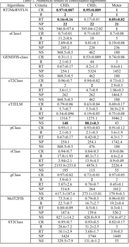
diagnosis. The RT2RVFLN was compared against 10 prominent algorithms: eT2Class [15], eClass [31], GENEFIS-class [23], eT2ELM [15], pClass [24], rClass [18], gClass [32], [33], McIT2FIS [34], ST2Class [22]. To ensure fair comparison, all algorithms are constructed in the MIMO architecture to output a final predicted class label. Five evaluation criteria, namely accuracy, the number of the fuzzy rule, the number of parameters and execution time and number of samples, are applied to evaluate the learning performance. All consolidated algorithms were executed under the same computational environments: Microsoft Surface Book with an Intel (R) Core (TM) i7–2600 CPU, 3.4 GHz processor, and 8 GB memory. Consolidated numerical results are served in Table 1.

Table 1. Numerical results of consolidated algorithms Algorithms Criteria CHD1 CHD2 Motor

RT2McRVFLN CR 0.97±0.007 0.95±0.009 1

R 2 2 1

RT 0.16±0.16 0.17±0.01 0.05±0.02

NP 22 22 21

NS 546.8±97.6 395.04±12.02 1 eClass1 CR 0.7±0.01 0.71±0.03 0.7±0.08

R 11.2±0.6 10 5

RT 2.09±0.8 0.81±0.1 0.19±0.08

NP 245.2 220 236

NS 868.5±0.5 462 180

GENEFIS-class CR 0.31±1.1 0.53±0.009 0.74±0.06

R 2.1±0.3 44 3

RT 0.67±0.17 4.2±1.5 0.6±0.1

NP 254.1 5324 1452

NS 868.5±0.5 462 180

eT2Class CR 0.96±0.7 0.94±0.02 0.73±0.3

R 2 2 2.9±0.3

RT 3.6±1.1 4.7±0.9 1.96±0.3

NP 262 262 1464.5

NS 868.5±0.5 462 180

eT2ELM CR 0.79±0.06 0.63±0.04 0.69±0.17 R 5.7±0.7 5.5±0.5 36.9±2.9 RT 0.34±0.096 0.19±0.05 0.75±0.08 NP 1316.7 1275.1 3946.2

NS 148 88.1±0.3 43

pClass CR 0.95±1.1 0.93±0.03 0.91±0.12 R 2.1±0.3 2.1±0.3 3.6±1.9 RT 0.67±0.17 0.42±0.2 4.3±1.7

NP 254.1 254.1 1742.4

NS 868.5±0.5 476 180

rClass CR 0.94±0.7 0.84±0.5 0.9±0.06 R 17.8±1.93 40.3±7.1 4.6±2.4 RT 3.94±2.1 13.9±4.5 0.9±0.49 NP 2153.8±233.8 4876.3 2226.4

NS 195 115 55

gClass CR 0.97±0.02 0.73±0.01 0.97±0.05

R 3.9±0.3 2 2

RT 5.07±2.6 0.78±0.7 0.45±0.1

NP 514.8 264 1012

NS 617.3±187.6 273.1±15.01 179.9±0.3 McIT2FIS CR 73.5±6.1 0.79±0.5 0.96±0.05 R 22.7±0.7 16.7±2.7 19.2±0.4 RT 0.88±0.09 0.5±0.1 0.3±0.1

NP 187.6 139.6 520.2

NS 827.1±14.2 428.8±9.9 174.4±47.2 ST2Class CR 0.95±0.7 0.93±0.5 0.82±0.17

R 28.6±7.2 31.2±2.5 3 RT 10.1±2.9 3.68±1.7 3.9±0.5

NP 3424 3744 1449

NS 329.5±7.9 131.4±1.2 55

CR: Classification Rate, HD: Hidden Node, RT: Runtime, NP: Network Parameters, NS: Number of Samples, CHD1: male, CHD2: Female.

Prediction of Coronary Heart Disease: the RT2McRVFLN was deployed to undertake the predictive analytics of coronary heart disease (Courtesy of Dr. Agus Salim, Melbourne, Australia). Our experiment was done using a dataset from a Nested-Case-Control (NCC) taking place within the SCHS cohort [27]. The predictive task was done for two different genders: Male and Female. 958 samples from male’s patients were collected where 298 of which represent cases, while 528 samples from female’s participants were obtained and 143 of which indicate cases. Participants in this study had no prior history of stroke nor coronary heart disease. Cases in the male and female samples here portrays incident acute myocardial infarction (AMI) or coronary heart disease death occurring until 31 December 2010. Ten input features were extracted based on consultation with medical experts. This problem constitutes a binary classification problem, where 1 depicts cases, whereas 0 delineates controls. The numerical study follows the 10-fold cross-validation procedure to avoid the data order dependency problem. Because of the random nature of the RT2McRVFLN, simulations were repeated five times and average results across five trials and 10-folds CV process are reported in Table 1. This is necessary to view a complete trend of the RT2McRVFLN performance.

It is observed in Table 1 that the RT2McRVFLN delivered the highest predictive accuracy while retaining the lowest complexity in terms of runtime, and number of parameters in the realm of the male dataset. The randomized learning procedure greatly affects the execution time of our algorithm because it leaves only few parameter learning scenarios during the training process – output weight. The cloud-based hidden node reduces the number of network parameters to be kept in the memory because it is parameter-free and requires no parameterization step. For the female dataset, the RT2McRVFLN still produced the most encouraging performance where it evolves the most compact and parsimonious network structure while sustaining the least misclassifications. While the simple-eTS experienced the fastest training speed, the predictive accuracy is still far below our algorithm.

Referring to Table 1, RT2McRVFLN achieved a perfect classification rate. It also imposed the lowest complexity on the other four evaluation criteria: the number of hidden nodes, run-time, the number of parameters, and the number of samples. Because the motor fault detection problem constituted a multi-class classification problem, all consolidated models were structured under the MIMO architecture where each output represented a particular target class. In the context of real-world motor fault diagnosis, the what-to-learn process using the active learning scenario plays a vital role because it is capable of relieving the operator’s annotation effort, which could be intractable in coping with life-long data streams.

V. CONCLUSION

A novel randomized neural network, namely Recurrent Type-2 Metacognitive Random Vector Functional Link Network (RT2McRVFLN) is proposed in this paper. The goal of RT2McRVFLN aims to solve four open problems of RNNs: uncertainty, temporal system dynamic, the sensitivity of system order and curse of dimensionality. The efficacy of the RT2McRVFLN was numerically confirmed using two real-world case studies featuring non-stationary characteristics and compared against ten state-of-the-art algorithms recently published in the literature. The RT2McRVFLN outperformed its counterparts in attaining a tradeoff between accuracy and simplicity. Our future work will be directed toward the algorithmic development of the ensemble learning approach to the evolving algorithms.

VI. REFERENCES

[1] L. Zhang, P.N. Suganthan, “ A Survey of Randomized Algorithms for Training Neural Networks”, Information Sciences, Vol.364-365, pp. 146-155, 2016.

[2] Pao, Y.-H. and Phillips, S. M, ” The functional link net and learning optimal control”, Neurocomputing, Vol.9(2), pp. 149–164, (1995).

[3] B. Igelnik, Y.H. Pao, “Stochastic choice of basis functions in adaptive function approximation and the functional-link net”, IEEE Transactions on Neural Networks, Vol.6(6), pp.1320-1329, 1995.

[4] F. Cao, Y. Tan, M. Cai, “ Sparse algorithms of Random Weight Networks and applications”, Expert Systems with Applications, Vol. 41, pp. 2457-2462, 2014.

[5] F. Cao, H. Ye, D. Wang, “ A probabilistic learning algorithm for robust modeling using neural networks with random weights”, Information Sciences, Vol.313, pp. 62-78, 2015.

[6] J. Zhao, Z. Wang, F. Cao, D. Wang, “ A local learning algorithm for random weights networks”, Knowledge-based Systems, Vol.74, pp. 159-166, 2015

[7] M. Alhandoosh, D. Wang, “ Fast decorrelated neural network ensembles with random weights”, Information Sciences, Vol.264, pp. 104-117, 2014 [8] S. Scardapane, D. Wang, M. Panella, A. Uncini, “ Distributed learning for Random Vector Functional-Link networks”, Information Sciences, Vol. 301, pp. 271-284, 2015.

[9] Y. Ren, P.N. Suganthan, N. Srinkanth, G. Amaratunga, “ Random Vector Functional Link Network for Short-term Electricity Load Demand Forecasting”, Information Sciences, doi:10.1016/j.ins.2015.11.039.

[10] W. Wan, Z. Zhou, J. Zhao, F. Cao, “ A novel face recognition method: Using random weight networks and quasi-singular value decomposition”, Neurocomputing, Vol. 151, pp. 1180-1186, 2015.

[11] K. Javed, R. Gouriveau, N. Zerhouni, “A New Multivariate Approach for Prognostics Based on Extreme Learning Machine and Fuzzy Clustering”, Vol. 45(12), pp. 2626-2639, 2015.

[12] P. Zhou, et al, “Multivariable dynamic modeling for molten iron quality using online sequential random vector functional-link networks with self-feedbackconnections ”, Information Sciences, Vol. 325, pp. 237-255, 2015.

[13] F.M. Pouzols, A. Lendasse, “Evolving fuzzy optimally pruned extreme learning machine for regression problems”, Evolving Systems, Vol.1, pp.43-58, 2010.

[14] B. Mirza, Z. Lin, N. Liu, “Ensemble of subset online sequential extreme learning machine for class imbalance and concept drift”, Neurocomputing, Vol.149, pp.315-329, 2015.

[15] M. Pratama, G. Zhang, M-J. Er, S. Anavatti, “ An Incremental Type-2 Meta-Cognitive Extreme Learning Machine”, IEEE Transactions on Cybernetics, online and inpress, 2016.

[16] P. Angelov, R. Yager, “ A new type of simplified fuzzy rule-based system”, pp. 1-21, 2011.

[17] Xiong,S., Azimi, J., Fern, X.Z,” Active Learning of Constraints for Semi-Supervised Clustering”,IEEE Transactions on Knowledge and Data Engineering, Vol.26(1), pp. 43-54, 2014.

[18] M.Pratama, J.Lu, S.Anavatti,” Recurrent Classifier based on An Incremental Meta-Cognitive-based Scaffolding Algorithm”, IEEE Transactions on Fuzzy Systems, Vol.23(2), pp. 369-386, 2015.

[19] H. Gan, et al., “Nonlinear Systems Modeling Based on Self-Organizing Fuzzy-Neural-Network with Adaptive Computation Algorithm “, IEEE Transactions on Cybernetics, Vol. 44(4), pp.554-564, (2014).

[20] J. Wang, P. Zhao, S. Hoi, R. Jin, “Online Feature Selection and Its Applications”, IEEE Transactions on Knowledge and Data Engineering, Vol. 26(3), pp. 698-710, 2014.

[21] I. Zliobaite, A. Bifet, B. Pfahringer, G. Holmes, “ Active Learning with Drifting Streaming Data”, IEEE Transactions on Neural Networks and Learning Systems, Vol.25, no.1, pp.27-39, 2014.

[22] M Pratama, J Lu, E Lughofer, G Zhang, S Anavatti, Scaffolding type-2 classifier for incremental learning under concept drifts, Neurocomputing, Vol.191, pp.304-329, 2016.

[23] M Pratama, SG Anavatti, E Lughofer, “Evolving fuzzy rule-based classifier based on GENEFIS”, in proceeding of 2014 IEEE International Conference on Fuzzy Systems, pp. 1-8, 2014.

[24] M.Pratama, et al., “ pClass:An Effective Classifier to Streaming Examples”, IEEE Transactions on Fuzzy Systems, Vol.23(2), pp.369-386, 2014.

[25] I.Y. Tyukin , D.V. Prokhorov , Feasibility of random basis function approximators for modeling and control, in: Proceedings of IEEE Conference on Control Applications & Intelligent Control, 2009, pp. 1391–1396. [26] W. Schmidt, M. Kraaijveld, R. Duin, Feedforward neural networks with random weights, in Proceedings of 11th IAPR International Conference on Pattern Recognition Methodology and Systems, 1992, pp. 1-4.

[27] Agus Salim, E Shyong Tai, Vincent Y Tan, Alan H Welsh, Reginald Liew, Nasheen Naidoo, Yi Wu, Jian-Min Yuan, Woon P Koh, Rob M van Dam, “ C-reactive protein and serum creatinine, but not haemoglobin A1c, are independent predictors of coronary heart disease risk in non-diabetic Chinese”, European journal of preventive cardiology, Vol. 23(12), pp. 1339-1349, 2016.

[28] M. Seera, C-P. Lim, D. Ishak, H. Singh, “Fault Detection and Diagnosis of Induction Motors Using Motor Current Signature Analysis and a Hybrid FMM–CART Model”, IEEE Transactions on Neural Networks and Learning Systems, Vol. 23(1), pp. 97-108, 2012.

[29] P. Angelov, Anomalous System State Identification, PCT application WO2013/171474, priority date 15 May 2012, GB1208542.9.

[30] P. Angelov, Machine Learning (Collaborative Systems), USA patent 8250004, granted 21 August 2012; priority date: 1 Nov. 2006; international filing date 23 Oct. 2007.

[31] P. Angelov, X. Zhou, “ Evolving Fuzzy Rule-Based Classifiers from Data Streams”, IEEE Transactions on Fuzzy Systems.

[32] Pratama, M., M-J. Er, Anavatti, S.G., Lughofer, E., Wang, N., Arifin,I., “ A novel meta-cognitive-based scaffolding classifier to sequential non-stationary classification problems”, In proceeding of 2014 International Conference on Fuzzy Systems, pp. 369-376, 2014

[33] M Pratama, J Lu, S Anavatti, E Lughofer, CP Lim, “An incremental meta-cognitive-based scaffolding fuzzy neural network”, Neurocomputing, Vol. 171, pp. 89-105, (2016)

[34] Das, A.K., Subramanian, K., Suresh, S., “ An Evolving Interval Type-2 Neurofuzzy Inference System and Its Metacognitive Sequential Learning Algorithm. IEEE Transactions on Fuzzy Systems, 23(6), pp. 2080-2093, (2015)