warwick.ac.uk/lib-publications
Manuscript version: Author’s Accepted Manuscript
The version presented in WRAP is the author’s accepted manuscript and may differ from the
published version or Version of Record.
Persistent WRAP URL:
http://wrap.warwick.ac.uk/92872
How to cite:
Please refer to published version for the most recent bibliographic citation information.
If a published version is known of, the repository item page linked to above, will contain
details on accessing it.
Copyright and reuse:
The Warwick Research Archive Portal (WRAP) makes this work by researchers of the
University of Warwick available open access under the following conditions.
Copyright © and all moral rights to the version of the paper presented here belong to the
individual author(s) and/or other copyright owners. To the extent reasonable and
practicable the material made available in WRAP has been checked for eligibility before
being made available.
Copies of full items can be used for personal research or study, educational, or not-for-profit
purposes without prior permission or charge. Provided that the authors, title and full
bibliographic details are credited, a hyperlink and/or URL is given for the original metadata
page and the content is not changed in any way.
Publisher’s statement:
Please refer to the repository item page, publisher’s statement section, for further
information.
Matthew Dobson
1, Manh Hong Duong
2, and Christoph Ortner
21
Department of Mathematics and Statistics, UMass Amherst, 710 N Pleasant
Street, Amherst, MA 01003, USA.
2
Mathematics Institute, University of Warwick, Coventry CV4 7AL, UK.
October 1, 2017
Abstract
We develop a rigorous error analysis for coarse-graining of defect-formation free energy. For a one-dimensional constrained atomistic system, we establish the thermodynamic limit of the defect-formation free energy and obtain explicitly the rate of convergence. We then construct a sequence of coarse-grained energies with the same rate but significantly reduced computational cost. We illustrate our analytical results through explicit computations for the case of harmonic potentials and through numerical simulations.
1
Introduction
Crystalline materials contain a variety of defects, such as vacancies, interstitials and disloca-tions. Macroscopic properties of materials are strongly dependent on the distribution of defects, in particular through the interaction between dislocations and other defects [CR10]. Meso-scopic models for defect interaction (e.g., dislocation dynamics, point defect diffusion) usually take as input an atomistic simulation of a single, or few defects, from which the meso-scopic model param-eters can be extracted. A prototypical example is the defect formation energy, which we discuss in more detail below. A great number of numerical schemes on spatial coarse-graining of the free en-ergy have been developed in the literature, see for instance in [DTMP05, MVH+10] and references therein. However, a rigorous analysis on the accuracy of these schemes is still underdeveloped; we are only aware of the references [BBLP10, SL14].
In this paper, we provide such a rigorous analysis for the computations of the defect-formation free energy. We consider one-dimensional constrained atomistic systems, which model perfect and defect materials respectively, with degrees of freedomu∈RN. The system can be either influenced
by external forces or not. In the case without external forces, free energies are respectively defined by
FN(A) =−β−1log
Z
RN−1
exph−βV(u)idu1. . . duN−1, (1)
FNP(A) =−β−1log
Z
RN−1
exph−βVP(u))idu1. . . duN−1, (2)
where
V(u) =
N
X
i=1
ψ(ui−ui−1), VP(u) =V(u) +P(u) (3)
are the energies associated to the perfect and defect materials, V is the sum of bond energies
ψ(ui−ui−1); P : RN → R models the defect. For simplicity, we assume thatP is a localised
function and depends only on the first bondP(u) =P(u1−u0); the analysis may be easily adapted
to the case of a defect in the bulk. Finally,β >0 is the inverse of the temperature.
In the case with external forces, the perfect free energy is unchanged, but the deformed free energy is influenced by the external forces
FNP(A) =−β−1log
Z
RN−1
exph−β
N
X
i=1
ψi(ui−ui−1)−βP(u1)
i
du1. . . duN−1, (4)
where ψi(y) =ψ(y) +hiy with {hi}Ni=1 representing the external forces. The forces are included
only in the defective energy in order to model a slowly decaying stress field surrounding a defect which is present in higher dimensions but not naturally present in the one dimensional case where elastic fields decay exponentially fast.
Note that the integrals (1), (2) and (4) are subjected to the boundary constraints
u0= 0, uN =N A (5)
so that the free energies depend onN andAas shown, andP(u) =P(u1).
The main quantity of interest in this paper is thedefect-formation free energy defined as the difference of the free energies
GN(A) :=FNP(A)−FN(A) =−
1
β log
R
RN−1exp(−βV
P(u))du
R
RN−1exp(−βV(u))du
. (6)
This quantity is used to obtain the equilibrium defect concentration [Put92, WSC11] or to analyse defect clustering [SK09, HKM+14]. A direct computation ofG
N(A) is practically impossible due
to the curse of dimensionality: one needs to compute integrals overRN−1, which is an extremely
high-dimensional space.
As a matter of fact, N itself is an approximation parameter, theexactdefect formation free energy is given by the thermodynamic limit, letting N → ∞. Establishing this limit, and thus making precise what we mean by the “exact model” is the first result of our paper. Once we have established this, we search for an alternative scheme by which to approximate it, which yields an improved accuracy/computational cost ratio.
The computation of limNGN is a problem that is interesting in its own right, but at the same
time it serves as a natural benchmark problem for exploring the relative accuracy/cost of coarse-graining methods at finite temperature. We introduce and analyze a coarse-coarse-graining approach based on the use of a finite temperature Cauchy-Born energy density.
The work [BBLP10] considers a similar model as ours, but this work is focused on the scaling limit of the free energy, not the free energy difference, which is a different scale. Furthermore, it does not take defects into account. The work [SL14] is in spirit much closer to ours and in particular does take defects into account. The main difference to our work is that [SL14] considers “low” temperature via an asymptotic series expansion. Moreover, our coarse-grained model has some close similarities with common quasicontinuum-type models.
Technically, to prove our main results, we will link the defect-formation free energy to a ratio of the densities of certain random variables and employ techniques from statistical mechanics. The latter have been used in the literature, for example in [GOVW09, Men11]. There is also a close relationship between our thermodynamic limit results and the Gibbs conditioning principle [DF88, DZ96]. We comment on this in Section 4. The connections to the defect-formation free energy, to the best of our knowledge, is new and moreover, some technical modifications of the mentioned papers were required.
1.1
Assumptions and main results
Assumption 1.1. ψ, P ∈C2(
R) and there exist positive constantsκ1≤κ2andς1≤ς2such that
κ1≤ψ00≤κ2, ς1≤(ψ+P)00≤ς2. (7)
Assumption 1.2. h:= (h1, h2. . .)∈l1; we can then defineH :=P∞i=2hi.
Step 1: Thermodynamic limit: Our first result concerns therate of convergenceof defect formation free energy. Its proof is given in Theorems 2.1 and 3.2.
Theorem 1.1. There existsG∞∈C∞(R), such that, for allA∈R
|GN(A)−G∞(A)|.N−1.
Step 2: Coarse-graining:
To motivate and put our work in the context of coarse-graining of thermodynamic quantities, we first recall its general set up. LetX =RN+M be a (microscopic) phase space endowed with a
probability (Boltzmann-Gibbs) measure
µ(dx) =Z−1exp(−E(x))dx.
We want to compute the average
A:=
Z
X
Φ(x)µ(dx)
of an observable Φ : X → R. Observables of interest are often functions of only part of the variable: forx= (y, z) withy∈RN, z∈
RM then Φ(x) = Φ(y, z) = Φ(y). In this case the average
above can be computed as an integral over a lower dimensional space,RN instead of
RN+M using
acoarse-grained energy Ecg:RN →R,
A=
Z
RN+M
Φ(y)µ(dy, dz) =
Z
RN
Φ(y)
Z
RM
Z−1exp(−E(y, z))dz
=
Z
RN
Φ(y) ˜Z−1exp(−Ecg(y))dy,
where the coarse-grained energyEcg is defined via
˜
Z−1exp(−Ecg(y)) =
Z
RM
Z−1exp(−E(y, z))dz.
However, it is often computationally intractable using the above definition. Instead, to compute
Ecgin practice, one views the problem as minimizing the Helmholtz free energy of the system with
y fixed, and approximating E(y, z) above. For example, in [DTMP05, TLK+13] the authors use
a local harmonic approximation along with a quasicontinuum-coarse grained mesh to compute an approximate free energyEcb(y, z)
Ecg(y) = inf
z∈RM
Ecb(y, z), (8)
for someEcb:
RN+M →R. This paper introduces a localized Cauchy-Born approximation in the
chain and justifies its use for the defect computation.
In our setting, the defect-formation free energy (6) can be written as an observable average as follows
GN(A) =−log
Z
RN−1
exp(−P)µN(du),
where µN(du) = Z−1exp(−V(u))du. Since the defect P is a localised function (in this paper,
P(u) = P(u1−u0)), we can apply the strategy described above to effectively compute GN(A).
N → ∞with explicit Ecb, and Theorem 1.3 computes the approximation errors. To state these
Theorems, we need to recall the Cauchy-Born strain energy which will appear throughout the rest of the paper.
The (finite-temperature) Cauchy-Born strain energy function is given by [BL13]
W(A) = sup
σ∈R
n
σA−log
Z
R
exp(−ψ(y) +σy)dyo. (9)
Taking a continuum model R[W(u0) +hu0]dxoutside the defect core {0,1} and then discretising it with the atomistic grid{1,2, . . . N}we obtain
ENcb(u) := N
X
i=2
h
W(u0i)−W(A) +hiu0i
i
, where u0i=ui−ui−1,
with admissible displacements u: {0, . . . , N} →R satisfyingu0 = 0, uN =AN. After replacing
ui=Ai+vi, summation by parts, and taking the formal limitN → ∞, yields
Ecb(u) =W0(A)(A−u1) +AH+
∞
X
i=2
h
W(A+vi0)−W(A)−W0(A)vi0+hivi0
i
.
It is important to note here that Ecb is formulated in a way that ensures it is well-defined for
arguments withv0∈`2.
We obtain the following characterisation ofG∞(A) in terms ofEcb.
Theorem 1.2. Let Ecg(A, y) := inf
u∈RN,u1=yEcb(u), then
G∞(A) =−log
R
Rexp −P(y)−ψ1(y)−E
cg(A, y)
dy
R
Rexp −ψ(y)−E
cg h=0(A, y)
dy .
whereEhcg=0 denotes the coarse-grained energy withhj ≡0.
In the absence of external forces, Theorem 1.2 can be derived from the Gibbs conditioning principle [DF88, DZ96]. However, it is not clear how to do so when there are external forces. We compare the technique we employ with the Gibbs conditioning principle in more details in Section 4.
Step 3: Approximation: Thus, we have replaced a limit of high-dimensional integrals by a one-dimensional integral over a coarse-grained energy functional whose evaluation requires the solution of an infinite-dimensional variational problem. In our next step, we replaceEcg(A, y) with a finite-dimensional approximation.
Let
ENcg(A, y) := inf
u∈RN u1=y,uN=N A
ENcb(u)
and
GcgN(A) :=−log
R
Rexp −P(y)−ψ1(y)−E
cg
N(A, y)
dy
R
Rexp −ψ(y)−E
cg
N,h=0(A, y)
dy .
Here we have chosenENcg as the most basic approximation scheme toEcg, but far more
sophisti-cated choices could be explored. With this definition we obtain the following result.
Theorem 1.3. (i)GcgN(A)is well-defined for all A∈R.
(ii) For allA∈R we have the estimate
G
cg
N(A)−G∞(A)
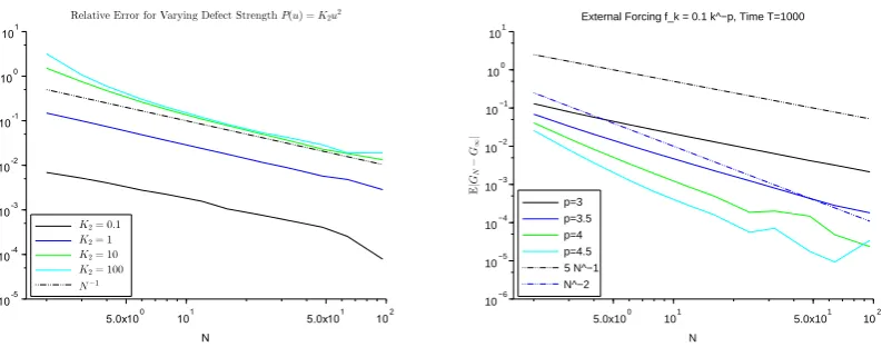
The sharpness of the results of Theorems 1.1 and 1.2 are demonstrated through explicit computations in the harmonic case ψ(y) =α|y|2 andP(y) =β|y|2 in Section 5 and in numerical
simulations in Section 6.
Interpretation: Statements (ii) of Theorems 1.2 and 1.3 imply that G∞(A) can be
com-puted from two one-dimensional integrals, but this extreme reduction of computational complexity is only due to the special one-dimensional structure of our model problem and cannot in general be reproduced.
The structure in our construction that can be expected more generally though is thatG∞(A)
can be approximated by a low-dimensional canonical average with respect to a coarse-grained energy that is obtained by a variational problem in the exterior of the computational domain. In our case the coarse-grained measure is one-dimensional but in general one may still expect it to be relatively low-dimensional. A Langevin or other type of Markov-Chain type algorithm can now be employed to computeG∞(A); cf. Section 6.
Of course, the evaluation of Ecg(y) is in general impossible, and an approximation needs to be performed. For example, ENcg(A, y) (and its derivatives) is computable with a reasonably low
O(N) cost. Note thatW itself may be costly to evaluate, but it could be easily precomputed to high accuracy e.g. via Taylor expansions or spline techniques. The O(N) cost could be reduced further if we employ a quasi-continuum style coarse-graining ofEcgN.
1.2
Organisation of the paper
The rest of the paper is structured as follows. In Section 2 we study the case without external forces. Extension to the case with external forces is shown in Section 3. In Section 4 we compare our work with Gibbs conditioning principle. In Section 5, we provide explicit computations for the harmonic case. Finally, in Section 6, we present some numerical simulations.
2
The case without external forces
In this section, we analyse the case without external forces.
2.1
Thermodynamic limit
In this section, we prove Theorem 1.1 for the case without external forces by establishing the existence of the thermodynamic limitG∞ and the rate of convergence ofGN toG∞. We give an
expression forG∞in terms of the Cauchy-Born strain energy (9), which arises here as in the Gibbs
conditioning principle, see Section 4. The main result of this section is the following theorem.
Theorem 2.1. Suppose that Assumption 1.1 is satisfied. Then the thermodynamic limit is given by
G∞(A) =−log
R
Rexp[−(ψ+P)(y) +W
0(A)y]dy
R
Rexp[−ψ(y) +W
0(A)y]dy . (10)
Moreover, for all A∈R, we have the estimate
|GN(A)−G∞(A)|.N−1. (11)
Proof. The proof is split into three steps that are Proposition 2.3, Proposition 2.7 and Proposition
2.10 below.
Lemma 2.2. Suppose that ψ˜i∈C2(R)and0< κ1≤ψ˜i00≤κ2 fori= 1, . . . , N. We define
˜
WN(A) = sup σ∈R
n
σA− 1
N N X i=1 log Z R
exp(−ψ˜i(y) +σy)dy
o
, (12)
˜
FN(A) =−log
Z
RN−1
exph−
N
X
i=1
˜
ψi(ui−ui−1)
i
du1. . . duN−1, (13)
withu0= 0, uN =N A.
Let σ∗ be the maximizer in (12). We define the one dimensional probability measures
˜
µσi∗(dy) =Zi−1exp(σ∗y−ψ˜i(y))dy, (14)
whereZiis the normalising constant. LetX˜ibe independent random variables distributed according
toµ˜σ∗
i and letm˜i be the mean of X˜i. Letg˜N,A be the density of √1N
N
P
i=1
( ˜Xi−m˜i). Then it holds
that
˜
FN(A) =
1
2logN+N ˜
WN(A)−log ˜gN,A(0). (15)
Proof. This proof is adapted from [Men11, Lemma 8] (see also [GOVW09, Eq. (125)]). By change
of variablesyi=ui−ui−1, fori= 1, . . . , N −1, we can re-write ˜FN(A) as
˜
FN(A) =−log
Z
RN−1
exp
"
−
N−1
X
i=1
˜
ψi(yi)−ψ˜N
N A−
N−1
X
i=1
yi
#
dy1. . . dyN−1. (16)
We define
˜
ϕN,i(σ) = log
Z
R
exp[−ψ˜i(y) +σy]dy,
˜
ϕN(σ) :=
1 N log Z RN exp − N X i=1 ˜
ψi(yi) +σ N
X
i=1
yi
dy1. . . dyN
then
(˜
WN(A) =σ∗A−ϕ˜N(σ∗),
A= d dσϕ˜N(σ)
σ=σ∗.
(17)
We have
˜
ϕN(σ) =
1 N log Z RN exp − N X i=1 ˜
ψi(yi) +σ N
X
i=1
yi
dy1. . . dyN
= 1 N N X i=1 log Z R
exp−ψ˜i(yi) +σyi
dyi = 1 N N X i=1 ˜
ϕN,i(σ). (18)
A straightforward calculation gives
˜
mi=
Z
R
yiµ˜σ
∗
i (dyi) =
d
dσϕ˜N,i(σ)
σ=σ∗. (19)
Substituting (18) and (19) into (17), we obtain
A= d
dσϕ˜N(σ)
σ=σ∗ =
1 N N X i=1 d
dσϕ˜N,i(σ)
σ=σ∗=
1 N N X i=1 ˜
Since ˜Xi are independent, the density of the sum P N
i=1X˜i is given by the convolution
˜
fPN
i=1Xi(ξ) = (˜µ
σ∗
1 ∗. . .∗µ˜
σ∗ N )(ξ).
Using the definition of convolution, we can compute the above density explicitly as follows
˜
fPN
i=1X˜i(ξ) =
Z
RN−1
exp − N X i=1 ˜
ϕN,i(σ∗) +σ∗ξ−ψ˜N(ξ− N−1
X
i=1
yi)− N−1
X
i=1
˜
ψi(yi)
dy1. . . dyN−1.
We recall that if Y has density f(y)dy then, for α > 0, β ∈ R, αY +β has density 1αf(y−αβ). Hence, we obtain
˜
gN,A(ξ) =f√1
N
PN
i=1( ˜Xi−mi)(ξ)
=√N
Z
RN−1
exp − N X i=1 ˜
ϕN,i(σ∗) +σ∗
ξ√N+
N X i=1 ˜ mi
−ψ˜N
√
N ξ−
N−1
X
i=1
yi+ N X i=1 ˜ mi −
N−1
X
i=1
˜
ψi(yi)
dy1. . . dyN−1.
In particular, using (18), (16) and (20), we get
˜
gN,A(0) =
√
N
Z
RN−1
exp − N X i=1 ˜
ϕN,i(σ∗) +σ∗ N
X
i=1
˜
mi−ψ˜N
−
N−1
X
i=1
yi+ N X i=1 ˜ mi −
N−1
X
i=1
˜
ψi(yi)
dy1. . . dyN−1
=√N
Z
RN−1
exp
−Nϕ˜N(σ∗) +σ∗N A−ψ˜N
N A−
N−1
X
i=1
yi
−
N−1
X
i=1
˜
ψi(yi)
dy1. . . dyN−1
=√Nexp[N(σ∗A−ϕ˜N(σ∗))]
Z
RN−1
exp
−ψ˜N
N A−
N−1
X
i=1
yi
−
N−1
X
i=1
˜
ψi(yi)
dy1. . . dyN−1
=√Nexp[N(σ∗A−ϕ˜N(σ∗))] exp[−F˜N(A)].
It follows from (17) and the above equality that
log ˜gN,A(0) =
1
2logN+N ˜
WN(A)−F˜N(A),
which is equivalent to (15) as claimed.
The following proposition provides an analytical expression of the defect-formation free energy in terms of densities of averages of independent random variables.
Proposition 2.3. Recall that the Cauchy-Born energy is given by
W(A) = sup
σ∈R
n
σA−log
Z
R
exp(−ψ(y) +σy)dyo. (21)
We define an analogous function that is associated to the defect material
WNP(A) = sup
σ∈R
σA− 1
N
log
Z
R
exp[−(ψ+P)(y) +σy]dy+ (N−1) log
Z
R
exp(−ψ(y) +σy)dy
.
Let σ0 andσNP be the maximisers in definitions of (21)and (22)respectively. We define the one-dimensional probability measures
µσ0(dy) =Z−1
µ exp(σ0y−ψ(y))dy, and (23)
νσPN(dy) =Z−1
ν exp(σPNy−(ψ+P)(y))dy, µσ
N
P(dy) =Z−1
µPexp(σ
N
Py−ψ(y))dy, (24)
whereZµ, Zν andZµP are normalising constants. Letm, mP,1 andmP,2 be respectively the means
of µσ0, νσNP(dy)andµσPN(dy).
Let {Xi}i=1,...,N and {Yi}i=1,...,N be independent random variables, where {Xi}i=1,...,N
dis-tributed according toµσ0(dy), {Y
1} distributed according to νσ
N
P(dy), and{Yi}i=2,...,N distributed
according to µσPN(dy). Let gN,A and gP
N,A be respectively the density of
1
√
N
PN
i=1(Xi−m) and
1
√
N
PN
i=1(Yi−mP,i)(withmP,2=. . .=mP,N).
Then it holds that
FNP(A)−FN(A) =N[WNP(A)−W(A)] + log
gN,A(0)
gP N,A(0)
. (25)
Proof. Applying Lemma 2.2 for the cases ˜ψi =ψ (i= 1, . . . , N) and ˜ψ1=ψ+P, ψ˜i =ψ (i=
2, . . . , N), we obtain the following relations respectively
FN(A) =
1
2logN+N WN(A)−loggN,A(0),
FNP(A) =
1
2logN+N W
P
N(A)−loggPN,A(0).
The assertion (25) immediately follows from these two relations.
The next step is to passing to the limitN → ∞for each term in the relation (25). We will need some auxiliary lemmas. We define
Ψ(σ) :=
R
Ryexp(−ψ(y) +σy)dy
R
Rexp(−ψ(y) +σy)dy
, (26)
Φ(σ) :=
R
Ryexp[−(ψ+P)(y) +σy]dy
R
Rexp[−(ψ+P)(y) +σy]dy
−
R
Ryexp(−ψ(y) +σy)dy
R
Rexp(−ψ(y) +σy)dy
.
The following lemma on boundedness of derivatives of Ψ and Φ will be used several times in the sequel.
Lemma 2.4. It holds that
1
κ2
≤ d
dσΨ(σ)≤
1
κ1
and
d dσΦ(σ)
≤C, (27)
for some positive constantC.
Proof. We first prove the first part of (27). The following proof is simplified from [Cap03, Lemma
2.4]. In [Cap03, Lemma 2.4] the author has actually proved a stronger result than we need here. We have
d
dσΨ(σ) =
R
Ry
2exp(−ψ(y) +σy)dy R
Rexp(−ψ(y) +σy)dy
− R
Ryexp(−ψ(y) +σy)dy
2 R
Rexp(−ψ(y) +σy)dy
2
=
Z
R
y−mσ
2
where
µσ(dy) :=
exp(−ψ(y) +σy)
R
Rexp(−ψ(y) +σy)dy
dy∈ P(R), and mσ=
Z
R
yµσ(dy).
Using this equality, we now estimate dσdΨ(σ) using assumptions onψ. For the upper bound: since
ψ00≥κ1,µσ satisfies the Poincare inequality with constantκ1uniformly inσ. Therefore,
d
dσΨ(σ)≤
1
κ1
Z
d dyy
2
µσ(dy) =
1
κ1
.
For the lower bound: using the inequalityg2≥2f g−f2for all functionsf andg, withg=y−m
σ,
we have
d
dσΨ(σ)≥
Z
[2f(y−mσ)−f2]µσ(dy).
By takingf =β(ψ0−σ) forβ∈R, and applying integration by parts, we obtain
d
dσΨ(σ)≥2β−β
2Z ψ00(y)µ
σ(dy).
Now maximizing overβ, by choosingβ= 1
R ψ00(y)µ
σ(dy), we get
d
dσΨ(σ)≥
1
R
ψ00(y)µ
σ(dy)
≥ 1
κ2
,
where we have used the assumption thatψ00≤κ2.
The second estimate in (27) is proved similarly. We have
d
dσΦ(σ) =
Z
R
(y−mPσ)2dµPσ(dx)−
Z
R
(y−mσ)2dµσ(dx), where
µPσ = R exp[−(ψ+P)(y) +σy]
Rexp[−(ψ+P)(y) +σy)dy
dy, and mPσ =
Z
R
yµPσ(dy).
Sinceψ+P satisfies a similar assumption asψ, we obtain
1
ς2
≤
Z
R
(y−mPσ)2dµPσ(dx)≤ 1
ς1
.
As a consequence, we get
1
ς2
− 1
κ1
≤ d
dσΦ(σ)≤
1
ς1
− 1
κ2
,
which implies the second estimate in (27).
We recall thatσ0andσNP are respectively maximisers in (21) and (22). The following lemma
provides an estimate for|σP N −σ0|.
Lemma 2.5. There exists a positive constantC such that, forN sufficiently large,
|σPN−σ0| ≤
C
N. (29)
Proof. SetF:= Ψ + 1
NΦ. Then we have
A= Ψ(σ0) =F(σNP), and F0(σ) = Ψ0(σ) +
1
NΦ
0(σ).
This, together with Lemma 2.4, imply that for sufficiently largeN and for allσ∈R
0.5
κ2
≤ |F0(σ)| ≤ 2
κ1
By the mean value theorem, there existsθ∈Rsuch that
F0(θ)(σPN−σ0) =F(σPN)−FP(σ0) =F0(σ0)−
F0(σ0) +
1
NΦ(σ0)
=−1
NΦ(σ0).
Hence
|σPN−σN0 |=
1
N
Φ(σ0)
F0(θ)
≤ C
N,
for some constantC >0 and for N sufficiently large.
The following estimate is elementary but will be used at various places later.
Lemma 2.6. For any z∈C, we have
|ez−1| ≤ |z|e|z|. (30)
Proof. We have
|ez−1|=
etz
1
0
=
Z 1
0
zetzdt
≤ |z|
Z 1
0
|etz|dt=|z|
Z 1
0
etRel(z)dt≤ |z|
Z 1
0
e|z|dt=|z|e|z|.
The second ingredient of the proof of Theorem 2.1 is the following proposition.
Proposition 2.7. It holds that
lim
N→∞N[W
P
N(A)−W(A)] =−log
R
exp[−(ψ+P)(y)−W0(A)y]dy
R
exp[−ψ(y)−W0(A)y]dy . (31)
Moreover, it hods that
N[WNP(A)−W(A)] + log
R
exp[−(ψ+P)(y)−W0(A)y]dy
R
exp[−ψ(y)−W0(A)y]dy
≤ C
N.
Proof. We recall thatσ0 and σPN are respectively the maximisers in the definitions ofW(A) and
WNP(A), so that
W(A) = sup
σ∈R
n
σA−log
Z
R
exp(−ψ(y) +σy)dyo (32)
=σ0A−log
Z
R
exp(−ψ(y) +σ0y)dy, (33)
whereσ0satisfies
A=
R
Ryexp(−ψ(y) +σ0y)dy
R
Rexp(−ψ(y) +σ0y)dy
= Ψ(σ0). (34)
By properties of the Legendre transform, we also haveW0(A) =σ
0, which is explicitly shown in
(62). Similarly
WNP(A) = sup
σ∈R
(
σA− 1
N
log
Z
R
exp[−(ψ+P)(y) +σy]dy+ (N−1) log
Z
R
exp(−ψ(y) +σy)dy
)
(35)
=σPNA−log
Z
R
exp[−ψ(y) +σNPy]dy− 1
N log
R
Rexp[−(ψ+P)(y) +σ N Py]dy
R
Rexp(−ψ(y) +σ N Py)dy
whereσN P solves
A= 1
N
R
Ryexp[−(ψ+P)(y) +σy]dy
R
Rexp[−(ψ+P)(y) +σy]dy
+N−1
N
R
Ryexp(−ψ(y) +σy)dy
R
Rexp(−ψ(y) +σy)dy
. (37)
Using these supremum representations we will estimate lower and upper bounds forN[WP N(A)−
W(A)]. For an upper bound: it follows from (32) that
WN(A)≥σPNA−log
Z
R
exp(−ψ(y) +σPNy)dy.
This, together with (36), we get
N[WNP(A)−W(A)]≤ −log
R
Rexp[−(ψ+P)(y) +σ N Py]dy
R
Rexp(−ψ(y) +σ N Py)dy
.
Similarly, using (35) and (33), we obtain
N[WNP(A)−W(A)]≥ −log
R
Rexp[−(ψ+P)(y) +σ0y]dy
R
Rexp(−ψ(y) +σ0y)dy
.
Bringing these bounds together,
−log
R
Rexp[−(ψ+P)(y) +σ0y]dy
R
Rexp(−ψ1(y) +σ0y)dy
≤N[WNP(A)−W(A)]≤ −log
R
Rexp[−(ψ+P)(y) +σ N Py]dy
R
Rexp(−ψ(y) +σ N Py)dy
.
(38) We now estimate the right-hand side of the last expression. We have
R
Rexp[−(ψ+P)(y) +σ N Py]dy
R
Rexp(−ψ(y) +σ N Py)dy
=
R
Rexp[−(ψ+P)(y) +σ0y+ (σ N
P −σ0)y]dy
R
Rexp[−(ψ+P)(y) +σ0y)dy
×
R
Rexp[−(ψ+P)(y) +σ0y]dy
R
Rexp(−ψ(y) +σ0y)dy
×
R
Rexp[−ψ(y) +σ0y]dy
R
Rexp[−ψ(y) +σ N Py]dy
=
R
Rexp[−(ψ+P)(y) +σ0y]dy
R
Rexp(−ψ1(y) +σ0y)dy
×
exp[(σNP −σ0)y]νσ0×
exp[(σNP −σ0)y]
−1
µσ0,
where
νσ0(y)dy= exp[−(ψ+P)(y) +σ0y] R
Rexp[−(ψ+P)(y) +σ0y)]dy
dy and µσ0(y)dy= exp[−ψ(y) +σ0y] R
Rexp[−ψ(y) +σ0y]dy
.
Taking the logarithm of the above equality, we deduce
−log
R
Rexp[−(ψ+P)(y) +σ N Py]dy
R
Rexp(−ψ(y) +σ N Py)dy
=−log
R
Rexp[−(ψ+P)(y) +σ0y]dy
R
Rexp(−ψ(y) +σ0y)dy
+ log
exp[(σPN−σ0)y]
νσ0 −log
exp[(σPN−σ0)y]
µσ0.
(39)
We now show that the last two terms in the right-hand side of (39) are of order O(N−1). Using
the estimate|et−1| ≤ |t|e|t| (Lemma 2.6) and Lemma 2.5, we have
|exp[(σPN −σ0)y]−1| ≤ |(σNP −σ0)y|exp(|(σPN −σ0)y|)≤
C
Therefore
exp[(σNP −σ0)y]νσ0−1 =
exp[(σPN−σ0)y]−1νσ0 ≤
|exp[(σPN−σ0)y]−1|νσ0
≤ C
Nh|y|exp(C|y|)iνσ0.
Since (ψ+P)(y) is bounded from below and above by a quadratic potential, it implies that the term
h|y|exp(C|y|)iνσ0 =
1
R
Rexp[−(ψ+P)(y) +σ0y]dy
Z
|y|exp[−(ψ+P)(y) +σ0y+C|y|]dy.
is finite. Therefore
exp[(σN
P −σ0)y]
νσ0 −1
≤ NC, which implies that
log
exp[(σNP −σ0)y]νσ0 ≤
C N.
Similarly, we obtain the following estimate for the last term in (39)
log
exp[(σPN−σ0)y]
µσ0 ≤
C N.
Substituting these above estimates to (39), we achieve the following estimate for the upper bound in (38) −log R
Rexp[−(ψ+P)(y) +σ N Py]dy
R
Rexp(−ψ(y) +σ N Py)dy
+ log
R
Rexp[−(ψ+P)(y) +σ0y]dy
R
Rexp(−ψ(y) +σ0y)dy
≤ C N.
Therefore, it follows from (38) that
N[WNP(A)−W(A)] + log
R
exp[−(ψ+P)(y)−σ0y]dy
R
exp[−ψ(y)−σ0y]dy
≤ C N.
This completes the proof of the proposition.
Next, we estimate the last term in (25). We will need two auxiliary lemmas.
Leth(m, ξ) :=hexp(iξ(x−m))iµσ, whereµσ(x)dx=Zσ−1exp(σx−ψ(x))dx.
Lemma 2.8. For any δ >0, it holds that
|h(m, ξ)| ≤1−1 2
p
Cσ 1−exp
− δ
2
2κ2
!
for |ξ| ≥δ, (40)
whereCσ= exp
σ2
4
κ1−κ2
κ1κ2 qκ
1
κ2.
Note that since 0< κ1< κ2, we have 0< Cσ<
qκ 1
κ2 <1, which is independent ofσ.
Proof. The proof of this lemma is adapted from that of [GOVW09, Lemma 39, (i)]. Sinceκ1x2≤
ψ(x)≤κ2x2, we have
µσ(x)≥ exp(σx−κ2x
2)
R
Rexp(σy−κ1y
2)dy =
exp(σx−κ2x2)
R
Rexp(σy−κ2y
2)dy
R
Rexp(σy−κ2y
2)dy
R
Rexp(σy−κ1y
2)dy =nσ(x)Cσ,
where
nσ(x) =
exp(σx−κ2x2)
R
Rexp(σy−κ2y
2)dy, Cσ=
R
Rexp(σy−κ2y
2)dy
R
Rexp(σy−κ1y
2)dy = exp
σ2
4
κ1−κ2
κ1κ2
rκ
1
κ2
Note that 0< Cσ<1 for allσ. The following identity is the same as [GOVW09, (157)]
|h(m, ξ)|2= 1−Var(cos(ξx))−Var(sin(ξx)). (41)
Next we estimate Var(cos(ξx)).
Var(cos(ξx)) =
Z
R
cos(ξx)−
Z
R
cos(ξy)µσdy
2
µσdy
≥Cσ
Z
R
cos(ξx)−
Z
R
cos(ξy)µσdy
2
nσ(x)
≥Cσ
" Z
R
cos(ξx)2nσ(dx)−
Z
R
cos(ξx)nσ(dx)
2#
. (42)
The second integral on the right-hand side can be computed explicitly as follows:
Z
R
cos(ξy)nσ(dy)
2 = 1 4 rκ 2 π exp − σ 2
4κ2
Z
R
[exp(iξx) + exp(−iξx)] exp(−κ2x2+σx)dx
2 = 1 4 r κ2 π exp iσξ
2κ2
Z
R
exp(iξy) exp(−κ2y2)dy+
r
κ2
π exp
−iσξ 2κ2
Z
R
exp(−iξy) exp(−κ2y2)dy
2 = 1 4 exp − ξ 2
4κ2
exp
iσξ
2κ2
+ exp
− ξ
2
4κ2
exp
−iσξ 2κ2
2 = 1 4exp − ξ 2
2κ2
exp iσξ κ2 + exp −iσξ κ2 + 2 = 1 2exp − ξ 2
2κ2
1 + cos(σξ
κ2
)
.
The first integral can be computed similarly:
Z
R
cos2(ξx)nσ(dx) =
1 2
1 + cos(σξ
κ2
) exp(−ξ
2 κ2 ) . Therefore, Z R
cos(ξx)2nσ(dx)−
Z
R
cos(ξx)nσ(dx)
2
= 1
2 1−exp
− ξ
2
2κ2
!
1−cos
σξ κ2 exp − ξ 2
2κ2
!
≥ 1
2 1−exp
−ξ2
2κ2
!2
.
Substituting these computations into (42) we obtain
Var(cos(ξx))≥1
2Cσ 1−exp
− ξ
2
2κ2
!2
.
By repeating the computation, we obtain that the same inequality holds for Var(sin(ξx)). There-fore,
|h(m, ξ)|2≤1−C
σ 1−exp
− ξ
2
2κ2
!2
If|ξ| ≥δ, then
|h(m, ξ)|2≤1−C
σ 1−exp
− δ
2
2κ2
!2
.
Since√1−x≤1−1
2x, it follows that
|h(m, ξ)| ≤1−1 2
p
Cσ 1−exp
− δ
2
2κ2
!
for |ξ| ≥δ.
This concludes the proof.
Define Λ(σ) := Var(µσ) =
R
R x−
R
Rx µσ(dx)
2
µσ(dx).
Lemma 2.9. There existsC >0 such that, for anyσ1, σ2∈R,
|Λ(σ1)−Λ(σ2)| ≤C|σ1−σ2|.
Proof. It follows from (28) that Λ(σ) = Ψ0(σ). According to [GOVW09, Lemma 41] we have
|Ψ00(σ)| ≤C,
for some constantC >0. As a consequence, we obtain that
|Λ(σ1)−Λ(σ2)|=|Ψ0(σ1)−Ψ0(σ2)| ≤C|σ1−σ2|.
This finishes the proof.
We are now ready to estimate the last term in the right-hand side of (25).
Proposition 2.10. There existsC >0 such that
logg
P N,A(0)
gN,A(0)
≤ C
N. (43)
Proof. We recall the general setting in Lemma 2.2.
˜
µσj∗(dy) = exp−ϕ˜N,j(σ∗) +σ∗y−ψ˜j(y)
dy,
where
˜
ϕj(σ) = log
Z
R
exp[−ψ˜j(y) +σ y]dy
For eachj = 1, . . . , N, let ˜mj and ˜ςj2 be the mean and variance of ˜µ σ∗ j , i.e.,
˜
mj =
Z
R
yµ˜σj∗(dy) and ς˜j2=
Z
R
(y−m˜j)2µ˜σ
∗
j (dy).
Then ˜gN,A has been defined to be the density of √1N P N
j=1( ˜Xj−mj), where ˜Xj are independent
random variables distributed according to ˜µσ∗ j .
Define ˜yj =yj −m˜j. The value of ˜gN,A at 0 can be expressed as (cf. e.g.,[GOVW09, Eq.
(127)],[Men11, Eq. (72)])
˜
gN,A(0) =
1 2π
Z
R N
Y
j=1
expiy˜j
1 √
N ξ
j
whereh·ij denotes the average with respect to ˜µσ
∗
j . For someδ >0 sufficiently small, we split the
above integral into two terms
Z R N Y j=1
expiy˜j
1 √ N ξ j dξ= Z n √1 Nξ ≤δ o N Y j=1 D
expiy˜j
1 √ N ξ E jdξ + Z n √1 Nξ ≥δ o N Y j=1 D
expiy˜j
1 √ N ξ E j dξ
= I + II,
so that
˜
gN,A(0) =
1
2π(I + II). (44)
According to [Men11, Proof of Theorem 4], the following estimates hold
0< C1≤ |I| ≤C2, and |II| ≤C3NλN−2, (45)
for some positive constantsC1, C2, C3and 0< λ <1 depending only onδ. The constantλis the
upper bound of hexp(iy˜jξ)ij
. Moreover, there exists a complex-valued functionhj(ξ) such that
for 0<|ξ|sufficiently small,
hexp(iy˜jξ)ij= exp(−hj(ξ)) with
hj(ξ)−
1 2˜ς
2
jξ
2
≤C|ξ|
3. (46)
We are now ready to prove Proposition 2.10. Applying (44), (45) and (46) for the perfect material, we have
gN,A(0) =
1
2π(I1+ II1),
where
I1=
Z n
√1Nξ ≤δ
oexp
−Nh(√ξ N)
dξ, (47)
0< C11≤ |I1| ≤C12, and |II1| ≤C13NλN1−2, (48)
for some 0< λ1<1 and positive constantsC11, C12, C13 and
h(ξ)−
1 2ς
2ξ2 ≤C|ξ|
3 for|ξ| 1
withς2denotes the variance of µσ0. According to Lemma 2.8, the constantλ
1is given by
λ1= 1−
1 2
p
Cσ0 1−exp
− δ
2
2κ2
!
,
with 0< Cσ0 <1. Similarly,
gPN,A(0) = 1
2π(I2+ II2), (49)
where
I2=
Z n
√1Nξ ≤δ
oexp −
N X j=1 ˜ hj ξ √ N !
dξ, (50)
0< C21≤ |I2| ≤C22, and |II2| ≤C23NλN2−2, (51)
for some 0< λ2<1 and positive constantsC21, C22, C23and
˜
h1(ξ)−
1 2ς
2
P,1ξ 2
≤C|ξ|
3, for |ξ| sufficiently small,
˜
h2=. . .= ˜hN, ςP,2=. . .=ςP,N,
˜
hj(ξ)−
1 2ς
2
P,jξ
2
≤C|ξ|
whereζ2
P,1 andζP,22 are respectively the variances ofνσ
N
P andµσ N P. The constantλ2is given by
λ2= max
(
1−1 2
q
CσN P
1−exp−δ
2
κ2
,1−1 2
q
˜
CσN P
1−exp− δ
2
κ2+ς2
)
,
with 0< CσN P,
˜
CσN P <1. Hence we obtain
gP N,A(0)
gN,A(0)
−1 = I2+ II2 I1+ II1
−1 = I2−I1 I1+ II1
+II2−II1 I1+ II1
. (52)
It follows from (48) that|I1+II1| ≤C forN sufficiently large, thus
gP N,A(0)
gN,A(0)
−1
≤ |I2−I1|+|II2−II1|. (53)
The second term decays exponentially fast since, from (48) and (51)
|II2−II1| ≤ |II1|+|II2| ≤CNλN−2, (54)
withλ= max{λ1, λ2}. It follows thatλ= 1−O(δ2).
It remains to estimate|I2−I1|. By changing variablet:= √ξN, we have
I1−I2=
Z n √1 Nξ ≤δ o " exp
−N h√ξ
N −exp − N X j=1 ˜ hj ξ √ N # dξ
=√N
Z δ
−δ
exp(−N h(t))−exp−
N
X
j=1
˜
hj(t)
dt = √ N Z δ −δ
exp−N h(t)
1−exp
N
X
j=1
(h(t)−˜hj(t))
dt. (55)
Note that
h(t)−
1 2Nζ
2t2
≤C
t3
N32 ,
˜
h1(t)−
1 2Nζ
2
P,1t 2
≤C
t3
N32 ,
˜
hj(t) =. . .= ˜hN(t), ζP,j =ζP,2 for j= 2, . . . , N, and
˜
hj(t)−
1 2Nζ
2
P,2t 2
≤C
t3
N32 ,
where we recall that ζ2, ζP,21 and ζP,22 are, respectively, the variances of µσ0, νσNP and µσNP. It follows that, fort <1,
exp −N h(t)
= exp
−1 2ζ
2t2
exp
−Nh(t)− 1 2Nζ
2t2
≤exp −1 2ζ
2t2
exp
Ct3 N12
≤exp
Ct2
N12
Now we estimate N X j=1
(h(t)−˜hj(t))
= N X j=1
h(t)− 1 2Nζ
2
t2+ 1 2Nζ
2
t2− 1 2Nζ
2
P,jt
2
+ 1 2Nζ
2
P,jt
2
−˜hj(t)
≤ N X j=1 h(t)−
1 2Nζ
2t2
+
1 2Nζ
2t2− 1
2Nζ
2 P,jt 2 + 1 2Nζ
2
P,jt
2−˜h
j(t)
≤Ct 3
N12
+N−1 2N
ζ2−ζP,22 t2+
1 2N
ζ2−ζP,21
t2. (57)
From Lemma 2.5 and Lemma 2.9, we have
ζ2−ζP,22 =
Λ(σ0)−Λ(σNP)
≤C|σ0−σPN| ≤
C N, and
|ζ2−ζP,21|=|ΛP(σNP)−Λ(σ0)| ≤ |ΛP(σPN)−ΛP(σ0)|+|ΛP(σ0)−Λ(σ0)| ≤
C N +C,
where ΛP(σ) is the variance of the measureZ−1Rexp[−(ψ+P)(x) +σx]dxand the last inequality
is obtained similarly as in Lemma 2.9.
Substituting these estimates into (57), we obtain that, fort <1,
N X j=1
(h(t)−˜hj)(t)
≤
Ct3
N12
+Ct
2
N + Ct2
N2 .
Ct2
N12 .
Therefore by using the estimate|ez−1| ≤ |z|e|z|, we obtain
1−exp
N X
j=1
(h(t)−h˜j(t))
≤ N X j=1
(h(t)−˜hj(t))
exp N X j=1
(h(t)−˜hj(t))
≤ Ct 2 √ N exp Ct2 √ N . (58)
Substituting the estimates (56)-(58) into (55), we obtain
|I1−I2| ≤
√
N
Z δ
−δ
expCt
2
N12 Ct2 √ N exp Ct2 √ N dt
≤CexpCδ
2
N12 Z δ
−δ
t2dt=O(δ3).
By choosingδ=N−α where 1 3 < α <
1 2 then
|II2−II1|.N λN .N(1−N−2α)N .N
e−N−2α
N
=N e−N−2α+1.N−1,
|I1−I2|.N−3α.N−1.
Substituting these estimates into (53), we obtain
gPN,A(0)
gN,A(0)
−1
.N−1,
implying that logg P N,A(0)
gN,A(0)
.N−1.
2.2
Coarse-grained energy
In this section, we prove Theorem 1.2 for the case without external forces by deriving the formula for the coarse-grained energy and the representation of the thermodynamic limitG∞(A).
We recall that the finite coarse-grained energyENcg is defined as a minimization problem
ENcg(A, y) := inf
u∈RN u1=y,uN=N A
N
X
i=2
[W(ui−ui−1)−W(A)]. (59)
Due to the separation of variables, which is a special property of the 1D model, the minimization is explicit (see Theorem 2.11 below and Theorem 3.1 for the case with external forces). This simplicity explains why the Cauchy-Born derivation from a continuum model leads to the correct coarse-grained energy in Theorem 1.2.
The main theorem of this section is the following.
Theorem 2.11. (i) The coarse-grained energy,Ecg(A, y) = lim
N→∞E
cg
N(A, y), exists and is given
by
Ecg(A, y) =W0(A)(A−y). (60)
In addition, for all A, y∈R we have|ENcg(A, y)−Ecg(A, y)|.N−1.
(ii) The defect formation free energy G∞(A)can be represented in terms of Ecg as
G∞(A) =−log
R
Rexp(−P(y)−ψ(y)−E
cg(A, y))dy
R
Rexp(−ψ(y)−E
cg(A, y))dy . (61)
Proof. We first prove (60). The minimizer of the minimization problem (59) satisfies the following
Euler-Lagrange equation
−W0(ui+1−ui) +W0(ui−ui−1) = 0,
which implies thatW0(ui−ui−1) =λ, i.e.,uN−uN−1=. . .=u2−u1(= (W0)−1(λ)). This implies
that
ui−ui−1=
1
N−1
N
X
j=2
(uj−uj−1) =
N A−y N−1 =A+
A−y N−1.
Thus, we obtain
ENcg(A, y) = (N−1)
WA+ A−y
N−1
−W(A)
.
By applying the mean value theorem twice, there exist 0≤θ, θ0≤1 such that
ENcg(A, y)−Ecg(A, y) = (N−1)
WA+ A−y
N−1
−W(A)
−W0(A)(A−y)
= (N−1)W0A+θA−y N−1
A−y
N−1−W
0(A)(A−y)
=
W0A+θA−y N−1
−W0(A)
(A−y)
=W00A+θ0A−y N−1
(A−y)2
N−1 .
Letx∈Rand letσxbe the maximiser in the definition ofW(x). Then we have
x= Ψ(σx) and W(x) =σxx−log
Z
R
It follows that
W0(x) =xdσx
dx +σx−Ψ(σx) dσx
dx =σx and W
00(x) = dσx
dx =
1 Ψ0(σ
x)
. (62)
According to Lemma 2.4, we have
|W00(x)| ≤C
for allx∈R. It implies that
W
00A+θ0A−y N−1
≤C and hence,
|ENcg(A, y)−Ecg(A, y)| ≤ C(A−y)
2
N−1 ,
which gives (60).
The representation (61) is a direct consequence of (10) and (60). Indeed,
G∞(A)
(10)
= −log
R
Rexp[−(ψ+P)(y) +W
0(A)y]dy
R
Rexp[−ψ(y) +W
0(A)y]dy
=−log
R
Rexp[−(ψ+P)(y)−W
0(A)(A−y)]dy
R
Rexp[−ψ(y)−W
0(A)(A−y)]dy
(60)
= −log
R
Rexp(−P(y)−ψ(y)−E
cg(A, y))dy
R
Rexp(−ψ(y)−E
cg(A, y))dy .
2.3
Propagation of error
In this section, we prove Theorem 1.3 for the case without external forces.
Proof of Theorem 1.3 for the case without external forces.
For shortening of the notation, we define ˜ψ:=ψ+P. We rewrite GcgN(A) as follows.
GcgN(A) =−log
R
exp[−ψ˜(y)−ENcg(A, y)]dy
R
exp[−ψ(y)−ENcg(A, y)]dy
=−log
R
exp[−ψ˜(y)−Ecg(A, y)]dy
R
exp[−ψ(y)−Ecg(A, y)]dy−log
R
exp[−ψ˜(y)−Ecg(A, y)−(Ecg
N(A, y)−Ecg(A, y))]dy
R
exp[−ψ˜(y)−Ecg(A, y)]dy
+ log
R
exp[−ψ(y)−Ecg(A, y)−(Ecg
N(A, y)−E
cg(A, y))]dy
R
exp[−ψ(y)−Ecg(A, y)]dy
=−log
R
exp[−ψ˜(y)−Ecg(A, y)]dy
R
exp[−ψ(y)−Ecg(A, y)]dy−log
D
exp[ENcg(A, y)−Ecg(A, y)]E
ζ1
+ logDexp[ENcg(A, y)−Ecg(A, y)]E
ζ2 ,
whereζ1andζ2 are two probability measures defined by
ζ1(y)dy=
exp[−ψ˜(y)−Ecg(y)]dy
R
exp[−ψ˜(y)−Ecg(y)]dy and ζ2(y)dy=
exp[−ψ(y)−Ecg(y)]dy
R
exp[−ψ(y)−Ecg(y)]dy.
We next show that the logarithmic terms are of orderO(N−1). The argument will be similar to
and using the estimate in Theorem 2.11, we get
|exp[ENcg(A, y)−Ecg(A, y)]−1| ≤ |ENcg(A, y)−Ecg(A, y)|exp[|ENcg(A, y)−Ecg(A, y)|]
≤ C
N(A−y)
2expC
N(A−y)
2
≤ C
N(A−y)
2expκ1+ς1
2 (A−y)
2, forN sufficiently large.
Therefore,
exp[EcgN(A, y)−Ecg(A, y)]
ζ1−1 =
exp[ENcg(A, y)−Ecg(A, y)]−1
ζ1
≤D exp[E
cg
N(A, y)−E
cg(A, y)]−1 E
ζ1
≤ C
N
D
(A−y)2expκ1+ς1
2 (A−y)
2E
ζ1 .
Thanks to Assumption 1.1, the last average term will be finite. Therefore,
exp[ENcg(A, y)−Ecg(A, y)]
ζ1−1 ≤
C N,
which implies that
logDexp[ENcg(A, y)−Ecg(A, y)]E
ζ1
≤ C
N.
Similarly we also have
logDexp[ENcg(A, y)−Ecg(A, y)]E
ζ2
≤ C
N.
Therefore, we obtain that
−log
R
exp[−ψ˜(y)−ENcg(y)]dy
R
exp[−ψ(y)−ENcg(y)]dy + log
R
exp[−ψ˜(y)−Ecg(y)]dy
R
exp[−ψ(y)−Ecg(y)]dy
≤ C
N.
This completes the proof.
3
External forces case
In this section, we consider the case where the external forces are present. Recall that in this case, the perfect free energy is unchanged as the external forces are used to model the decay rate of the defect away from the core. The perfect material energy is given by
(
FN(A) =−β−1log
R
RN−1exp
h
−βPN
i=1ψ(ui−ui−1)
i
du1. . . duN−1
u0= 0, uN =N A.
(63)
The deformed free energy is influenced by the external forces
(
FNP(A) =−β−1logR
RN−1exp
h
−βPN
i=1ψi(ui−ui−1)−βP(u1)
i
du1. . . duN−1
u0= 0, uN =N A,
(64)
whereψi(y) =ψ(y)+hiy. The defect-formation free energy is defined as the free energy difference,
G∞(A) := limN→∞GN(A), where
GN(A) =FNP(A)−FN(A). (65)
Finally, the finite-domain coarse-grained energy is given by
ENcg(A, y) := inf
u∈RN u1=y,uN=N A
N
X
i=2
h
W(ui−ui−1)−W(A) +hi(ui−ui−1)
i
. (66)
Recall also that the external forces{hi}ni=1 satisfy Assumption 1.2 andH =
P∞
3.1
Coarse-grained energy
We now establish the formula for the coarse-grained energy, thus proving Theorem 1.2 for the case with external forces.
Theorem 3.1. The coarse-grained energy, Ecg(A, y) := lim
N→∞E
cg
N(A, y), is given by
Ecg(A, y) = (A−y)W0(A) +AH+ inf
v∈RN v1=0
J∞(A;v), (67)
where
J∞(A;v) = ∞
X
i=2
[W(A+vi0)−W(A)−W0(A)vi0+hivi0]. (68)
In addition, for all A, y∈R, we have the estimate
|ENcg(A, y)−Ecg(A, y)|.N−1+A| ∞
X
i=N+1
hi|+
∞
X
i=N+1
|hi|2. (69)
Proof. By changing variablesvi0=u0i−Aand substituting to (66), we obtain
ENcg(A, y) = inf
v∈RN v1=y−A,vN=0
IN(A;v), (70)
where
IN(A;v) = N
X
i=2
[W(A+vi0)−W(A) +hi(vi0+A)]
=
N
X
i=2
[W(A+vi0)−W(A)−W0(A)v0i+hiv0i] +A N
X
i=2
hi+ (A−y)W0(A)
=JN(A;v) +A N
X
i=2
hi+ (A−y)W0(A),
with
JN(A;v) = N
X
i=2
[W(A+v0i)−W(A)−W0(A)v0i+hiv0i]. (71)
Therefore
ENcg(A, y) =A
N
X
i=2
hi+ (A−y)W0(A) + inf v∈RN v1=y−A,vN=0
JN(A;v). (72)
We now show that
lim
N→∞ v∈infRN v1=y−A,vN=0
JN(A;v) = inf v1=y−A
J∞(A;v), (73)
where
J∞(A;v) = ∞
X
i=2
[W(A+vi0)−W(A)−W0(A)vi0+hivi0].
In fact, sinceJ∞(A;v) depends only onv0i, we have that
inf
v∈RN v1=y−A
J∞(A;v) = inf
v∈RN v1=0
To shorten the notation, we define Θi(A, z) =W(A+z)−W(A)−W0(A)z+hizso that
JN(A;v) = N
X
i=2
Θ(A, v0i), and J∞(A;v) = ∞
X
i=2
Θi(A, vi0).
A minimizer ofJ∞(A; ) satisfies the following Euler-Langrange equation fori= 2, . . . , N
Θ0i(A;v0i) = 0,
together with the boundary condition v1 =y−A. In particular, since Θ0i(A, z) =W0(A+z)−
W0(A) +h
i=W00(A+θz)z+hi for some θ∈R, it follows that
|vi0|= |hi| |W00(A+θv0
i)|
≤ |hi|
κ1
.
We define an admissible sequence ˜vi as follows
˜
v1=y−A, v˜N = 0, v˜i0=vi0+CN,
for someCN. Since {v0i} ∈ l
1, we havePN
i=2v0i →afor somea∈R. By summing up the above
equalities, it follows that
|CN|.
|y−A|+|a|
N .
Sincevi0 minimizes Θi we have
0≤Θi(˜vi0)−Θi(vi).CN2 .N
−2.
As a consequence, we obtain
inf
w∈RN w1=y−A,wN=0
JN(A;w)≤JN(A; ˜v)
=JN(A;v) + N
X
i=2
[Θi(˜vi0)−Θi(vi0)]
≤J∞(A;v) +CN−1+ ∞
X
i=N+1
Θi(vi0)
≤J∞(A;v) +CN−1+C ∞
X
i=N+1
|hi|2. (74)
Note that in the estimation above we have used the fact that|Θi(vi0)| ≤C(|hi|2+|vi0|
2)| ≤C|h
i|2.
On the other hand, using again the fact thatv0i minimizes Θi for eachi= 2, . . . , N, we have
inf
w∈RN w1=y−A,wN=0
JN(A;w)≥JN(A;v) =J∞(A;v)− ∞
X
i=N+1
Θ(vi0)≥J∞(A;v)−C ∞
X
i=N
|hi|2. (75)
From (74) and (75), we obtain
inf
v∈RN v1=y−A,vN=0
JN(A;v)− inf v∈RN v1=y−A
J∞(A;v)
.N
−1+
∞
X
i=N+1
|hi|2, (76)
from which (73) follows. Finally, from (72) and (76), we get
|ENcg(A, y)− lim
N→∞E
cg
N(A, y)|.N
−1+A
∞
X
i=N+1
hi
+
∞
X
i=N+1
|hi|2,
3.2
Thermodynamic limit
The main result of this section is the following theorem on the representation of the defect formation free energy.
Theorem 3.2. The thermodynamic limit is given by
G∞(A) =−log
R
Rexp[−(ψ1+P)(y)−E
cg(A, y)]dy
R
Rexp[−ψ(y)−E
cg
h=0(A, y)]dy
. (77)
whereEcg(A, y)is defined in (67).
Proof of Theorem 3.2. The proof is analogous to that of Theorem 2.1 which consists of three main
steps.
Step 1) Express the defect-formation free energy in terms of the energy difference and a ratio of the densities of random variables based on Lemma 2.2.
Step 2) Establish the limit of the energy difference.
Step 3) Show that the ratio of the densities of random variables are of orderO(1/N).
We now only sketch out the main computations in Step 1) and Step 2). Applying Lemma 2.2 for the case ˜ψ1=ψ1+P,ψ˜2=ψi, fori= 2, . . . , N to obtain
WNP(A) = sup
σ∈A
n
σA− 1
N log
Z
R
exp[−(ψ1(y) +P(y) +σy]dy−
1
N log
Z
R N
X
i=2
exp[−ψi(y) +σy]dy
o
,
=σNA−
1
N log
Z
R
exp[−(ψ1(y) +P(y) +σNy]dy−
1
N log
Z
R N
X
i=2
exp[−ψi(y) +σNy]dy.
The optimal valueσN solves
A= 1
N
R
Ryexp[−(ψ1(y) +P(y)) +σy]dy
R
Rexp[−(ψ1(y) +P(y)) +σy]dy
+ 1
N
N
X
i=2
R
Ryexp[−ψi(y) +σy]dy
R
Rexp[−ψi(y) +σy]dy
= 1
NΨP(σ−h1) +
1
N
N
X
i=2
Ψ(σ−hi), (78)
where Ψ is defined in (26) and ΨP is given by
ΨP(σ) =
R
Ryexp[−(ψ1(y) +P(y)) +σy]dy
R
Rexp[−(ψ1(y) +P(y)) +σy]dy
. (79)
SinceW(A) is unchanged, it is the same as in (32)-(33), so that
N[WNP(A)−W(A)] =N(σN−σ0)A−log
R
Rexp[−(ψ1(y) +P(y)) +σNy]dy
R
Rexp[−ψ(y) +σ0y]dy
−
N
X
i=2
log
R
Rexp[−ψi(y) +σNy]dy
R
Rexp[−ψ(y) +σ0y]dy
=N(σN−σ0)A−log
R
Rexp[−(ψ1(y) +P(y)) +σNy]dy
R
Rexp[−ψ(y) +σ0y]dy
−
N
X
i=2
[W∗(−hi+σN)−W∗(σ0)], (80)
where σ0 =W0(A). We will need the following lemma whose proof is postponed after the proof
Lemma 3.3. It holds that
|σN −σ0| ≤
C
N. (81)
To proceed, we will compare this free energy difference with the finite-domain coarse-grained energy. Recalling that the latter is defined by (see (66)),
ENcg(y) := inf
u:{1,N}→R u(1)=y,u(N)=N A
N
X
i=2
h
W(ui−ui−1)−W(A) +hi(ui−ui−1)
i
=A
N
X
i=2
hi+ inf u:{1,N}→R u(1)=y,u(N)=N A
N
X
i=2
h
W(ui−ui−1) +hi(ui−ui−1)−(hiA+W(A))
i
. (82)
The Euler-Lagrange equation for a minimizer ofENcg is
−W0(ui+1−ui) +W0(ui−ui−1)−(hi+1−hi) = 0,
which implies that
W0(ui−ui−1) =−hi+λ
for i = 2, . . . , N and for some λ ∈ R. We note that (W0)−1(z) = (W∗)0(z), where W∗ is the
Legendre transformation ofW. It follows from the definition ofW that
W∗(x) = log
Z
exp[−ψ(z) +xz]dz,
and so
(W∗)0(x) =
R
xexp[−ψ(z) +xz]dz
R
exp[−ψ(z) +xz]dz = Ψ(x).
Therefore, we obtain that
ui−ui−1= (W0)−1(−hi+λ) = (W∗)0(−hi+λ) = Ψ(−hi+λ).
Summing up these equalities from i= 2 toN and using the boundary condition on u, we obtain the following equation forλ=λN
N A−y=
N
X
i=2
Ψ(−hi+λN). (83)
Next, we use the following relations of the Legendre transform
W(x) =W0(x)x−W∗(W0(x)), W0((W∗)0(x)) =x
to obtainW(A) =W0(A)A−W∗(W0(A)) and
W(ui−ui−1) =W((W∗)0(−hi+λN))
=W0((W∗)0(−hi+λN))(W∗)0(−hi+λN)−W∗(W0((W∗)0(−hi+λN)))
Therefore, the sum inside the inf in (82) can be re-written as (recalling thatuN =N A, u1=y)
N
X
i=2
h
W(ui−ui−1) +hi(ui−ui−1)−hiA−W(A)
i
=
N
X
i=2
h
(−hi+λN)(W∗)0(−hi+λN)−W∗(−hi+λN) +hi(W∗)0(−hi+λN)
−hiA−W0(A)A+W∗(W0(A))
i
=λN N
X
i=2
(W∗)0(−hi+λN)− N
X
i=2
h
W∗(−hi+λN)−W∗(W0(A)) +hiA+W0(A)A
i
=λN N
X
i=2
(ui−ui−1)−
N
X
i=2
h
W∗(−hi+λN)−W∗(W0(A)) +hiA+W0(A)A
i
=λN(N A−y)−A N
X
i=1
hi−(N−1)W0(A)A− N
X
i=2
h
W∗(−hi+λN)−W∗(W0(A))
i
.
Substituting this expression back into (82), we get
EcgN(y) =λN(N A−y)−(N−1)W0(A)A− N
X
i=2
[W∗(−hi+λN)−W∗(W0(A))]
=λN(A−y) + (N−1)(λN −W0(A))A− N
X
i=2
[W∗(−hi+λN)−W∗(W0(A))]. (84)
It follows from (80) and (84) that
N[WN(A)−W(A)]−E
cg
N(A) = (σN −σ0)A−log
R
Rexp[−(ψ1(y) +P(y)) +σNy]dy
R
Rexp[−ψ(y) +σ0y]dy
+
N
X
i=2
([σNA−W∗(−hi+σN)]−[λNA−W∗(−hi+λN)])
= (σN −σ0)A−log
R
Rexp[−(ψ1(y) +P(y)) +σNy]dy
R
Rexp[−ψ(y) +σ0y]dy
+bN(σN)−bN(λN), (85)
where
bN(x) := N
X
i=2
[xA−W∗(−hi+x)].
Then we have
b0N(x) = (N−1)A−
N
X
i=2
(W∗)0(−hi+x),
b00N(x) =−
N
X
i=2
(W∗)00(−hi+x) =− N
X
i=2
Ψ0(−hi+x)≤0,
Furthermore, from (83) and (78), we have
b0N(λN) = (N−1)A− N
X
i=2
(W∗)0(−hi+λN) =y−A,
b0N(σN) = (N−1)A− N
X
i=2
(W∗)0(−hi+σN) = ΨP(σN−h1)−A.
Since dσd ΨP(σ)≤κ11+ς1, we have
|ΨP(σN −h1)| ≤ |ΨP(0)|+
1
κ1+ς1
|σN −h1| ≤ |ΨP(0)|+
1
κ1+ς1
(|σ0−h1|+|σN−σ0|)
≤
|ΨP(0)|+
1
κ1+ς1
(|σ0−h1|+C)
.
Therefore bothb0
N(λN) andb0N(σN) are uniformly bounded. It follows that
|bN(σN)−bN(λN)|=|σN −λN||b0N(θN)|
≤ |σN −λN|max{|b0N(σN), b0N(λN)|}
≤C|σN−λN|
≤C[|σN−W0(A)|+|λN−W0(A)|]
≤C(N−1)−1.
Substituting this estimate into (85), we obtain
N[WN(A)−W(A)]−
ENcg(A) + (σN−σ0)A−log
R
Rexp[−(ψ1(y) +P(y)) +σNy]dy
R
Rexp[−ψ(y) +σ0y]dy
≤ C
N.
(86) An analogous argument as in the proof of Proposition 2.7 we obtain
log
R
Rexp[−(ψ1(y) +P(y)) +σNy]dy
R
Rexp[−ψ(y) +σ0y]dy
−log
R
Rexp[−(ψ1(y) +P(y)) +σ0y]dy
R
Rexp[−ψ(y) +σ0y]dy
≤ C
N. (87)
The assertion (77) of Theorem 3.2 is then followed from (86), Theorem 3.1, Lemma 3.3 and (87).
We now prove Lemma 3.3.
Proof of Lemma 3.3. DefineL(σ) := N1ΨP(σN) +N1 P
N
i=2Ψ(σN −hi). Then we have
A= Ψ(σ0) =L(σN).
Hence,
L(σN)−L(σ0) = Ψ(σ0)−L(σ0) =
1
N(Ψ(σ0)−ΨP(σ0−h1)) +
1
N
N
X
i=2
(Ψ(σ0)−Ψ(σ0−hi)).
By the mean value theorem, there existsθ such that
L(σN)−L(σ0) =L0(θ)(σN −σ0). (88)
We have
|L0(θ)||σN −σ0|=|L(σN)−L(σ0)| ≤
1
N
"
|Ψ(σ0)−ΨP(σ0−h1)|+
N
X
i=2
|Ψ(σ0)−Ψ(σ0−hi)|
#
≤ 1
N
"
|Ψ(σ0)−ΨP(σ0−h1)|+
1
κ1
N
X
i=2
|hi|
#