Original citation:
Cormode, Graham, Dasgupta, Anirban, Goyal, Amit and Lee, Chi Hoon. (2018) An evaluation of multi-probe locality sensitive hashing for computing similarities over web-scale query logs. PLoS One, 13 (1). e0191175.
Permanent WRAP URL:
http://wrap.warwick.ac.uk/97688
Copyright and reuse:
The Warwick Research Archive Portal (WRAP) makes this work of researchers of the University of Warwick available open access under the following conditions.
This article is made available under the Creative Commons Attribution 4.0 International license (CC BY 4.0) and may be reused according to the conditions of the license. For more details see: http://creativecommons.org/licenses/by/4.0/
A note on versions:
The version presented in WRAP is the published version, or, version of record, and may be cited as it appears here.
An evaluation of multi-probe locality sensitive
hashing for computing similarities over
web-scale query logs
Graham Cormode1☯*, Anirban Dasgupta2☯, Amit Goyal3☯, Chi Hoon Lee3☯
1 Department of Computer Science, University of Warwick, Coventry, United Kingdom, 2 Computer Science and Engineering, IIT Gandhinagar, Gandhinagar, India, 3 Yahoo Research, Sunnyvale CA, United States of America
☯These authors contributed equally to this work. *[email protected]
Abstract
Many modern applications of AI such as web search, mobile browsing, image processing, and natural language processing rely on finding similar items from a large database of com-plex objects. Due to the very large scale of data involved (e.g., users’ queries from commer-cial search engines), computing such near or nearest neighbors is a non-trivial task, as the computational cost grows significantly with the number of items. To address this challenge, we adopt Locality Sensitive Hashing (a.k.a, LSH) methods and evaluate four variants in a distributed computing environment (specifically, Hadoop). We identify several optimizations which improve performance, suitable for deployment in very large scale settings. The exper-imental results demonstrate our variants of LSH achieve the robust performance with better recall compared with “vanilla” LSH, even when using the same amount of space.
1 Introduction
Every day, hundreds of millions of people visit web sites and commercial search engines to pose queries on topics of their interest. Such queries are typically just a few key words intended to specify the topic that the user has in mind. To provide users with a high quality service, search engines such as Bing, Google, and Yahoo require intelligent analysis to realize users’ implicit intents. The key resource that they have to help tease out the intent is their large his-tory of requests, in the form of large scale query logs, as well as the log of user actions on the corresponding result pages. A key primitive in learning users’ intents is finding the nearest neighbors for a user-given query. Computing nearest neighbors is useful for many search-related problems on the Web and Mobile such as finding search-related queries [1–3], finding near-duplicate queries [4], spelling correction [5,6], and diversifying search results [7]; and Natural Language Processing (NLP) tasks such as paraphrasing [8,9], calculating distributional simi-larity [10–12], and creating sentiment lexicons from large-scale Web data [13].
In this paper, we focus on the problem of finding nearest neighbors over very large data sets, and ground our study with the application of searching for the best match of a given
a1111111111 a1111111111 a1111111111 a1111111111 a1111111111 OPEN ACCESS
Citation: Cormode G, Dasgupta A, Goyal A, Lee CH (2018) An evaluation of multi-probe locality sensitive hashing for computing similarities over web-scale query logs. PLoS ONE 13(1): e0191175.
https://doi.org/10.1371/journal.pone.0191175
Editor: Yeng-Tseng Wang, Kaohsiung Medical University, TAIWAN
Received: May 5, 2017
Accepted: December 3, 2017
Published: January 18, 2018
Copyright:©2018 Cormode et al. This is an open access article distributed under the terms of the
Creative Commons Attribution License, which permits unrestricted use, distribution, and reproduction in any medium, provided the original author and source are credited.
Data Availability Statement:Deidentified AOL
data is available from the figshare repository
https://doi.org/10.6084/m9.figshare.5527231.v1
QLogs data is proprietary and cannot be released by us. Requests to access this data can be addressed to Yahoo’s academic relations manager,
query from very large scale query logs from a large search engine. In order to understand the implicit users’ intent, each query is initially represented in a high dimensional feature space, where each dimension corresponds to a clicked url. Given the importance of this question, it is critical to design algorithms that can scale to many queries over huge logs, and allow online and offline computation. However, computing nearest neighbors of a query can be very costly. Naive solutions that involve a linear search of the set of possibilities are simply infeasible in these settings due to the computational cost of processing hundreds of millions of queries. Even though distributed computing environments such as Hadoop make it feasible to store and search large data sets in parallel, the naive pairwise computation is still infeasible. The rea-son is that the total amount of work performed is still huge, and simply throwing more resources at the problem is not effective. Given a log of hundreds of millions queries, most are “far” from a query of interest, and we should aim to avoid doing many “useless” comparisons that only confirm that other queries are indeed far from it.
In order to address the computational challenge, this paper aims to find nearest neighbors by doing asmallnumber of comparisons—that is, sublinear in the dataset size—instead of brute force linear search. In addition to minimizing the number of comparisons, we aim to retrieve neighboring candidates with 100% precision and high recall. It is important that the false positive rate (ratio of “incorrectly” identifying queries as close) is penalized more severely than the false negative rate (ratio of missing “true” neighbors).
When seeking exact matches for queries, effective solutions are based on storing values in a hash table and mapping in via hash functions. The generalization of this approach to approxi-mate matches is the framework of Locality Sensitive Hashing, where queries are more likely to collide under the hash function if they are more alike, and less likely to collide if they are less alike. The methods we propose in this paper meet our criteria by extending Locality Sensitive Hashing [14–16]. In particular, we apply the framework within a distributed system, Hadoop, and take advantage of its distributed computing power.
Our work makes the following contributions:
1. We describe four variants of vanilla LSH motivated by the research on Multi-Probe LSH [17]. We show that two of these achieve much better recall than vanilla LSH using the same number of hash tables. The main idea behind these variants is to intelligently probe multi-ple “nearby” buckets within a table that have high probability of containing near neighbors of a query.
2. We present a framework on Hadoop that efficiently finds nearest neighbors for a given query from commercial large-scale query logs in sublinear time.
3. We discuss the applicability of our framework on two real-world applications: finding related queries and removing (near) duplicate queries. The algorithms presented in this paper are currently being implemented for production use within a large search provider.
2 Problem statement
We start with user query logsChaving query vectors collected from a commercial search engine over some domain (e.g. URLs); closeness of queries is measured via cosine similarity on the corresponding vectors. Given a set of queriesQand similarity thresholdτ, the problem is to develop a batch process to return asmallsetTof candidate neighbors fromCfor each queryq2Qsuch that:
1. T= {ljs(l,q)τ,l2C}, wheres(q1,q2) is a function to compute a similarity score between query feature vectorq1andq2;
any role in the development and execution of this work. The work of AD, AG, CHL was carried out while they were employed by Yahoo Research. Yahoo provided the query log data used to evaluate the compared methods. The funder provided support in the form of salaries for authors AD, AG, CHL, and computing resources, but did not have any additional role in the study design, data analysis, decision to publish, or preparation of the manuscript. The specific roles of these authors are articulated in the ‘author contributions’ section.
2. Tachieves 100% precision with “large” recall. That is, our aim is to achieve high recall, while using a scalable efficient algorithm.
The exact brute force algorithm to solve the above problem would be to computes(l,q) for allq2Qand alll2Cand return those (l,q) wheres(l,q)>τ. This approach is computationally infeasible on a single machine, even if the size ofQis of the order of few thousands when the size ofCis hundreds of millions. Even in a distributed setting such as Hadoop, the resulting communication needed between machines makes this strategy impractical.
Our aim is to study locality sensitive hashing techniques that enable us to return a set of candidate neighbors while performing a much smaller (sublinearin |Q|×|C|) set of compari-sons. In order to tackle this scalability problem, we explore the combination of distributed computation using a map-reduce platform (Hadoop) as well as locality sensitive hashing (LSH) algorithms. We explore a few commonly known variants of LSH and suggest several variants that are suitable to the map-reduce platform. The methods that we propose meet the practical requirements of a real life search engine backend, and demonstrates how to use local-ity sensitive hashing on a distributed platform.
3 Proposed approach
We describe a distributed Locality Sensitive Hashing framework based on map-reduce. First, we present the “vanilla” LSH algorithm due to Andoni and Indyk [16]. This algorithm builds on prior work on LSH and Point Location in Equal Balls (PLEB) [14,15]. Subsequent prior work on new variants of PLEB [18] for distributional similarity can be seen as implementing a special case of Andoni and Indyk’s LSH algorithm. We next present four variants of vanilla LSH motivated by the technique of Multi-Probe LSH [17]. A significant drawback of vanilla LSH is that it requires a large number of hash tables in order to achieve good recall in finding nearest neighbors, making the algorithm memory intensive. The goal of Multi-probe LSH is to get significantly better recall than the vanilla LSH with the same number of hash tables. The main idea behind Multi-probe LSH is to look up multiple buckets within a table that have a high probability of containing the nearest neighbors of a query. We present the high-level ideas behind the Multi-probe LSH algorithm; for more details, the reader is referred to [17].
3.1 Vanilla LSH
The LSH algorithm relies on the existence of a family of locality sensitive hash functions. LetH
be a family of hash functions mappingRDto some universe S. For any two query termsp,q,
we chooseh2Huniformly at random and analyze the probability thath(p) =h(q). Supposed
is a distance function (e.g. cosine distance),R>0 is a distance threshold, andc>1 an approxi-mation factor. LetP1,P22(0, 1) be two probability thresholds. The familyHof hash functions is called a (R,cR,P1,P2) locality sensitive family if it satisfies the following conditions:
1. Ifd(p,q)R, then Pr[h(p) =h(q)]P1,
2. Ifd(p,q)cR, then Pr[h(p) =h(q)]P2
An LSH family is generally interesting whenP1>P2. However, the difference betweenP1 andP2can be very small. Given a familyHof hash functions with parameters (R,cR,P1,P2), the LSH algorithm amplifies the gap between the two probabilitiesP1andP2by concatenating Khash functions to createg() as:g(q) = (h1(q),h2(q),. . .,hK(q)). A larger value ofKleads to a
larger gap between probabilities of collision for close neighbors (i.e. distance less thanR) and those for neighbors that are far (i.e. distance more thancR); the corresponding probabilities arePK
probability of dissimilar queries having the same hash value. To increase therecallof the LSH algorithm, Andoni et al. useLhash tables, each constructed using a differentgj() function,
where eachgj() is defined asgj(q) = (h1,j(q),h2,j(q),. . .,hK,j(q)));81jL.
Algorithm 1 Locality Sensitive Hashing Algorithm
Preprocessing: Input is N queries with their respective feature vectors.
• Select L functions gj, j = 1, 2, . . ., L, setting gj(q) = (h1,j(q), h2, j(q), . . ., hK,j(q)), where {hi,j, i 2 [1, K], j 2 [1, L]} are chosen at random from the LSH family.
• ConstructL hash tables, 81 j L. All queries with the same gj value (81 j L) are placed in the same bucket.
Query: Set of M test queries. Let q denote a test query. • For each j = 1, 2, . . ., L
– Retrieve all the queries from bucket gj(q)
– Compute cosine similarity between query q and all retrieved que-ries. Return all the queries within thresholdτ.
3.2 LSH for cosine similarity
For cosine similarity we adapt the LSH family defined by Charikar [15]. The cosine similarity
between two queriesp;q2RD
is kppkk:qqk
. The LSH functions for cosine similarity use a
ran-dom vectora2RDto define a hash function ashα(p) = sign(αp). A negative sign is
inter-preted as 0 and positive sign as 1 to generate indices of buckets in the hash tables (i.e. the range of eachgj) asKbit vectors. To createα, we exploit the intuition in [19] and sample each
coordi-nate ofαfrom {−1, +1} with equal probability. In practice, these are generated by hash func-tions that maps that index to {−1, +1} (a.k.a. the “hashing trick” of [20]). This lets us avoid explicitly storing a (huge)D×K×Lrandom projection matrix.
Algorithm 1 gives the algorithm for creating and querying the data structure. In a prepro-cessing step, the algorithm takes as inputNqueries along with the associated feature vectors. In our application, each query is represented using an extremely sparse and high dimensional feature vector constructed as follows: for queryq, we take all the webpages (urls) that any user has clicked on when querying forq. Using this representation, we generate theLdifferent hash values for each queryq, where each such hash value is again the concatenation ofKhash func-tions. TheseLhash values per query are then used to createLhash tables. Since the width of the index of each bucket isKand each coordinate is one bit, each hash table contains 2K buck-ets. Each query term is placed in its respective buckets in each of theLhash tables.
To retrieve near neighbors, we first find all query terms appearing in the buckets associated with each of theMtest queries. We compute cosine similarity between each of the retrieved terms and the input test queries and return all those queries as neighbors which are within a similarity threshold (τ).
larger thanτ, ensuring that our precision is 100%. To only consider matches between theM
test queries and theNstored queries, we simply tag each query with its type (test or stored), and only consider candidate pairs that have one of each type. Our experiments show that this map-reduce implementation scales to hundreds of millions of queries.
3.3 Reusing hash functions
Directly implementing vanilla LSH requiresL×Khash functions. But generating hash tions is computationally expensive as it takes time to read all features and evaluate hash func-tions over all those features to generate a single bit. To reduce the number of hash funcfunc-tions evaluations, we use a trick from Andoni and Indyk [16] in which hash functions are reused to generateLtables.Kis assumed to be even andRpffiffiffiL. We generatefj(q) = (h1,j(q),h2,j(q),. . .,
hK/2,j(q))) of lengthk/2. Next, we defineg(q) = (fa,fb), where 1a<bR. Using such
pair-ings, we can thus generateL¼RðR21Þhash indices. This scheme requiresOðKpffiffiffiL) hash func-tions, instead ofO(KL). We use this trick to generateLhash tables with bucket indices of widthKbits.
3.4 Multi-Probe LSH
Since generating hash functions can be computationally expensive and the memory required by the algorithm scales linearly withL, the number of hash tables, it is desirable to keepL
small. The large memory footprint of vanilla LSH makes it impractical for many real applica-tions. Here, we first describe four new variants of the vanilla LSH algorithm motivated by the intuition in Multi-probe LSH [17]. Multi-probe LSH obtains significantly higher recall than vanilla LSH while using the same number of hash tables. The main intuition for Multi-probe LSH is that in addition to looking at the hash bucket that a test queryqfalls in, it is also possi-ble to look at the neighboring buckets in order to find its near neighbor candidates. Multi-probe LSH in [17] suggests exploring neighboring buckets in order of their Hamming distance from the bucket in whichqfalls. They show (empirically) that these neighboring buckets con-tain the near neighbors with very high probability. Though Multi-probe LSH achieves higher recall for the same number of hash tables, it makes more probes as it searches multiple buckets per table. The advantage of searching multiple buckets over generating more tables is that less memory and time is required for table creation.
The original Multi-probe LSH algorithm was developed for Euclidean distance. However, that algorithm does not immediately translate to our setting of cosine similarity. For example, in generating the list of other buckets inspected, [17] utilizes the distance of the hash value to the bucket boundary—this makes sense when the hash value is a real number, but we have bits. We present four variants of Multi-probe LSH for cosine similarity:
• Random Flip Q: Our baseline version first computes the initial LSH of a test queryqto give theLbucket ids. Next, we createFalternate bucket ids by flipping a set of coordinates ran-domly in eachgj(q). For scalability, we restrict our implementation to flipping a single bit
out of theKpossible bits each time, and ensure that the sampling is done without repetition. Since the hash functions are randomly chosen, we implement this by simply flipping the first bit, then revert it and flipping the second bit, until we reach theF’th bit.
is a one-time operation done while creating the database. We generate up toFvariants of each hash, so for each query, first itsLLSH representations of lengthKare generated. On each of theLrepresentations, flipping of bits is appliedFtimes to generateLF representa-tions of a query.
• Distance Flip Q: The third variant is a smarter version of Random Flip Q. It selects coordi-nates based on thedistanceofqfrom the random hyperplane (hash function) used to create this coordinate. The distance of the test queryqfrom the random hyperplaneαis the abso-lute value which we get before applying the sign function on it (see Section 3.2), i.e., abs(α
q), the distance ofqfrom hyperplaneα. This method flips up toFcoordinates in order of increasing distance from the hyperplane. That is, for each group ofKhash values, we sort by the distance to the hyperplane, and swap each of the firstFof these in turn. As with Random Flip Q, we restrict to flip only a single bit in each repetition, soFK.
• Distance Flip B: Our fourth variant flips bits for both the test query and for the queries in the database (i.e., the intelligent version of the second baseline). Like Random Flip B, it rquires us to flip all database items, which is a one-time data pre-processing step.
The map-reduce implementation of Multi-probe LSH follows the same structure as the vanilla one—the map phase of the first map-reduce job generates the alternate bucket-ids for both the test query and the queries in the database. For all LSH methods, the first preprocess-ing step is the same, which is to evaluate the hash functions to generateKpffiffiffiLbits. The second step is to generate tables indexed by the hash function id and bucket id. Within the map job, each query is mapped to its various indices. For multiprobe LSH, each query is also mapped to additional indices. Within the reduce job, all queries with the same index are collected and all colliding pair of queries (that share the same index) are output. The final step is to compute similarity for the colliding pairs and only keep those pairs that are above the thresholdτ(based on exact comparison using their original feature representation).
3.5 Time cost
The exact running time of these algorithms is hard to predict, as it depends on the distribution of the data, as well as the configuration of the computing environment (number of machines, communication topology etc.). Broadly speaking, the time cost is comprised of the preprocess-ing (the one-time cost to build the database of queries), and the runtime cost to process a new set of query look-ups. The communication cost of our algorithms in the Map-Reduce frame-work is low, since the majority of the frame-work is embarassingly parallel. Across all our methods, at mostOðKpffiffiffiLÞhash function evaluations are needed. While it may seem that the multiprobe LSH methods require more hash function evaluations, we aim to choose the parametersKand
Lso that less work is needed overall in order to achieve the same level of recall compared to the vanilla LSH methods. The final step, to compute the true similarity of the retrieved pairs, is proportional to the number of collisions. We expect the proposed methods to be faster here, since there should be fewer candidates to test. This stands in contrast to the naive exact method, which performs an all-pairs comparison.
4 Experiments
4.1 Data
We use two data sources for our experiments. The first is theAOL-logsdataset that contains search queries posed to the AOL search engine and that dataset was made available in 2006 [21]. This data is accessible from the figshare repository,https://doi.org/10.6084/m9.figshare. 5527231.v1. We also use a partial sample of query logs from a commercial search engine, denoted as Qlogs. Note that realistic query log information is considered confidential and con-tains potentially sensitive information about individuals. We are therefore careful in our han-dling of the data, and report only aggregate results and carefully chosen examples. We do not have permission to share the Qlogs data further, but to allow reproduction of results we show all our analyses on the public data. We were provided access to this data on request to Yahoo via an electronic file. Requests for access to this data can be addressed to Yahoo’s academic relations manager, mailto:[email protected].
As Qlogs reaches hundreds of millions of queries (approximately 600Munique queries), we generated multiple datasets from Qlogs by sampling at various rates:Qlogs001represents a 1% sample,Qlogs010represents a 10% sample andQlogs100represents the entire Qlogs. The smaller datasets are primarily used to explore parameter ranges and identify suitable val-ues that we then use to experiment with the larger dataset. For each queryq, a feature vector in a high dimensional feature space, denoted as q = (f1,f2, ,fD), was created by settingfito be
the click through rate of urliwhen shown in the search results page of search-queryq. Note that in our real implementation, q is represented as a sparse feature vector with only non-zero click-through rate features being present. In a pre-processing step, we remove all queries with at most five clicked urls.Table 1summarizes the statistics of our query-log datasets.
Test Data. In all experiments we use a randomly sampled set of 2000 queriesQ, as the test set. That is, we want to find setT, whereT= {ljs(q,q0)τ},s(q,q0) is cosine similarity, andq0
2CforC2{Qlogs001, Qlogs010, Qlogs100, AOL-logs}. For most experiments, we set the similarity thresholdτ= 0.7, meaning that forq, candidatesq0
having cosine similar-ity of larger than or equal to 0.7 are retrieved.
Evaluation Metrics. We use two metrics for evaluation: recall and number of comparisons. The recall of an LSH algorithm measures how well the algorithm can retrieve thetruesimilar candidates. The number of comparisons performed by an algorithm is computed as the aver-age number of pairwise comparisons done per test query, and measures the total computation done. The aim is to maximize recall and to minimize the number of comparisons.
4.2 Evaluating vanilla LSH
First, we vary the similarity threshold parameterτin the range {0.7, 0.8, 0.9} while fixing
K= 16 andL= 10 for theAOL-logsandQlogs001datasets.Table 2shows thatτ= 0.9 achieves higher recall thanτ= 0.7. This is expected as finding near duplicates is actually easier
Table 1. Query-logs statistics.
Data N D
AOL-logs 0.3×10⁶ 0.7
×106
Qlogs001 6×10⁶ 66×106
Qlogs010 62×106 464×106
Qlogs100 617×106 2.4
×109
than finding near neighbors that satisfy only a looser similarity criterion. For the rest of this paper,τis set as 0.7 since it represents the more challenging case.
In the second experiment, we varyRto be in {1, 4, 7, 10}, corresponding to values ofLof {1, 10, 28, 55}, while fixingK= 16 on theAOL-logsandQlogs001datasets. Recall thatL
denotes the number of hash tables andKis the width of the index of the buckets in the table. IncreasingKresults in increasing precision of the candidate pairs by reducing false positives, butLneeds to be correspondingly increased in order to maintain good recall (i.e. reduce false negatives).Table 3shows that increasingLleads to better recall, at the cost of more compari-sons on both datasets. In addition, largeLmeans generating many random projection bits and hash tables which is both time and memory intensive. Hence, we fixL= 10, to achieve reason-able recall with a tolerreason-able number of comparisons.
Next, we varyKin {4, 8, 16} while fixingL= 10. As expected,Table 4shows that increasing
Kreduces the number of comparisons and worsens recall on both datasets. This is intuitive as the larger value ofKleads to larger gap between probabilities of collision for queries that are close and those that are far. Henceforth, we fixK= 16 to have an acceptable number of comparisons.
In the fourth experiment, we fixL= 10 andK= 16 as determined above, and we increase the size of training data.Table 5demonstrates that as we increase data size, the number of comparisons done by the algorithm also increase. This result indicates thatKneeds to be Table 2. Varyingτwith fixedK= 16 andL= 10.
τ AOL-logs Qlogs001
Comparisons Recall Comparisons Recall
0.7 57 .63 1052 .67
0.8 .84 .81
0.9 .98 .96
https://doi.org/10.1371/journal.pone.0191175.t002
Table 3. VaryingLwith fixedK= 16 andτ= 0.7.
L AOL-logs Qlogs001
Comparisons Recall Comparisons Recall
1 7 .28 106 .36
10 57 .63 1052 .67
28 152 .77 2908 .78
55 297 .89 5648 .84
https://doi.org/10.1371/journal.pone.0191175.t003
Table 4. VaryingKwith fixedL= 10 withτ= 0.7.
K AOL-logs Qlogs001
Comparisons Recall Comparisons Recall
4 112,347 .98 2,29,2670 .96
8 11,008 .90 221,132 .88
16 57 .63 1,052 .67
tuned with respect to a specific dataset, as a largerKwill reduce the probability of dissimilar queries falling within the same bucket.KandLcan be tuned by randomly sampling a small set of queries. In this paper, we randomly select 2000 queries to tune parameterK.
Table 6shows the best choices ofKfor our datasets. We note that onQlogs100the preci-sion/recall cannot be computed, as it was computationally infeasible to find the exact similar neighbors. On our biggest dataset of 600M queries, we setK= 24 andL= 10. These settings require only 464 comparisons (on average) to find approximate neighbors compared to exact cosine similarity that involves brute force search over all 600M queries.
4.3 Evaluating multi-probe LSH
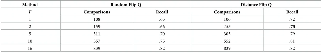
First, we compare flippingFbits in the query only. We evaluate two approaches: Random Flip Q and Distance Flip Q. We make several observations fromTable 7: 1) As expected, increasing the number of flips improves recall at the expense of more comparisons for both Distance Flip Q and Random Flip Q. 2) The last row ofTable 7shows that when we flip allKbits (F= 16), Distance Flip Q and Random Flip Q converge to the same algorithm, as expected. 3) We see that Distance Flip Q has significantly better recall than Random Flip Q with a similar number of comparisons. In the second row of the table withF= 2, the recall of Distance Flip Q is nine points better than that of Random Flip Q.
Table 5. FixedK= 16 andL= 10 withτ= 0.7.
Data Comparisons Recall
AOL-logs 57 .63
Qlogs001 1,052 .67
Qlogs010 10,515 .64
Qlogs100 105,126
-https://doi.org/10.1371/journal.pone.0191175.t005
Table 6. Best parameter settings ofK(minimizing comparisons and maximizing recall) withL= 10.
Data Comparisons Recall
AOL-logs(K= 16) 57 .63
Qlogs001(K= 16) 1,052 .67
Qlogs010(K= 20) 695 .53
Qlogs100(K= 24) 464
[image:10.612.34.581.600.691.2]-https://doi.org/10.1371/journal.pone.0191175.t006
Table 7. Flipping the bits in the query only withK= 16 andL= 10 onAOL-logswithτ= 0.7.
Method Random Flip Q Distance Flip Q
F Comparisons Recall Comparisons Recall
1 108 .65 106 .72
2 159 .66 155 .75
5 311 .70 303 .79
10 557 .75 552 .81
16 839 .82 839 .82
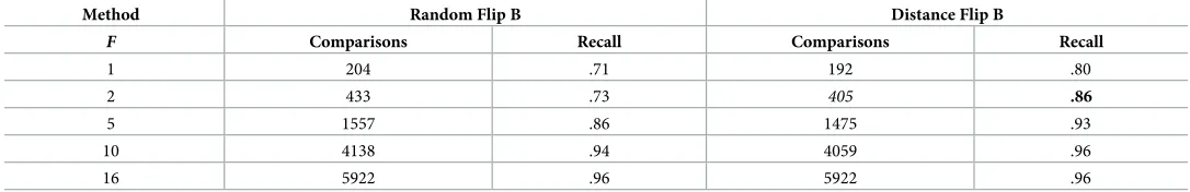
Table 8shows the result of flippingFbits in both query and the database. In the second row ofTable 8withF= 2, Distance Flip B has thirteen points better recall than Random Flip B with a similar number of comparisons. Comparing across the second row of Tables7and8shows that flipping bits in both query and database has better recall at the expense of more compari-sons. This is expected as flipping both means that we increase our “radius of search” to include queries at distance two (one flip in query, one flip in database), and hence have more queries in each table when we probe. We also compared distance-based flipping with random flipping on different input sizes, and found that distance-based flipping always has much better recall compared to random flipping (for brevity, we omit these numbers).
[image:11.612.38.586.241.320.2]We selectF= 2 as the best parameter setting with goal of maximizing recall by restricting comparisons to a minimum. For better recall at the expense of more comparisons,F= 5 can also be selected. However, results in Tables7and8indicate thatF>5 doesnotincrease recall significantly while leading to more comparisons.
Table 9gives the results of both variants of distance-based Multi Probe, i.e. Distance Flip Q and Distance Flip B, on different sized datasets. We present results with the parametersL= 10,
F= 2, and value ofKchosen as per the values used in the final vanilla LSH experiment. As observed there, flipping bits in both query and the database is significantly better in terms of recall with more comparisons. The second and third row of the table respectively shows that flipping bits in both query and the database has eight points better recall on bothQlogs001
andQlogs010datasets. With the goal of maximizing recall with some extra comparisons, we select Distance Flip B as our preferred algorithm. Distance Flip B maximizes recall with few tables and comparisons. On our entire corpus (Qlogs100) with hundreds of millions of que-ries, Distance Flip B only requires 3,427 comparisons per test query, compared to hundreds of millions of comparisons by the exact brute force algorithm. Distance Flip B returns 9 neigh-bors on average per given query, averaged over 2000 random test queries. Here, many queries are long, and have few neighbors.
Table 8. Flipping the bits in both the query and the database withK= 16 andL= 10 onAOL-logswithτ= 0.7.
Method Random Flip B Distance Flip B
F Comparisons Recall Comparisons Recall
1 204 .71 192 .80
2 433 .73 405 .86
5 1557 .86 1475 .93
10 4138 .94 4059 .96
16 5922 .96 5922 .96
https://doi.org/10.1371/journal.pone.0191175.t008
Table 9. Best parameter settings ofK(minimizing comparisons and maximizing recall) withL= 10,F= 2,τ= 0.7.
Method Distance Flip Q Distance Flip B
Data Comps. Recall Comps. Recall
AOL-logs(K= 16) 155 .75 405 .86
Qlogs001(K= 16) 2980 .76 7904 .84
Qlogs010(K= 20) 1954 .64 5242 .72
Qlogs100(K= 24) 1280 - 3427
4.4 Discussion
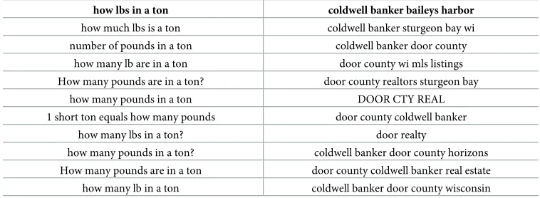
Tables10and11shows some qualitative results for a set of arbitrarily chosen queries. These results are found by applying our system (Distance Flip B with parametersL= 10,K= 24, and
F= 2) onQlogs100. These results help to highlight several applications that can take signifi-cant advantage of the approximate Distance Flip B algorithm presented in this paper. For example, the second column inTable 10shows that the returned approximate similar neigh-bors can be useful in finding related queries [1,2]. The first column inTable 11shows an example where we find several popular spelling errors automatically, which can usefully be used for query suggestion.
[image:12.612.198.577.98.237.2]One interesting application of near-neighbor finding is to understand specific intents behind the user query. Given a user’s query, Bing, Google, and Yahoo often delivers direct dis-play results that summarize expected contents of the query. For instance, when a query “f stock price” is issued to search engines, the quick summary of the stock quote with a chart is delivered to the user as the part of the search engine result page. Such direct display results are expected to reduce the number of unnecessary clicks by providing the user with the appropri-ate content early on. However, when the query “f today closing price” is issued to search engines, the three major search engines fail to deliver the same direct display experience to the Table 10. 10 similar neighbors returned by Distance Flip B withL= 10,K= 24, andF= 2 onQlogs100for two example queries.
how lbs in a ton coldwell banker baileys harbor
how much lbs is a ton coldwell banker sturgeon bay wi
number of pounds in a ton coldwell banker door county
how many lb are in a ton door county wi mls listings
How many pounds are in a ton? door county realtors sturgeon bay
how many pounds in a ton DOOR CTY REAL
1 short ton equals how many pounds door county coldwell banker
how many lbs in a ton? door realty
how many pounds in a ton? coldwell banker door county horizons
How many pounds are in a ton door county coldwell banker real estate
how many lb in a ton coldwell banker door county wisconsin
[image:12.612.199.578.547.687.2]https://doi.org/10.1371/journal.pone.0191175.t010
Table 11. 10 similar neighbors returned by Distance Flip B withL= 10,K= 24, andF= 2 onQlogs100for two example queries.
michaels trumbull ct weather
maichaels trumbull ct weather forecast
machaels weather in trumbull ct
mechaels weather in trumbull ct 06611
miachaels trumbull weather forecast
michaeils trumbull ct 06611
michaelos trumbull weather ct
michaeks trumbull ct weather report
michaeels trumbull connecticut weather
michaelas weather 06611
michae;ls weather trumbull ct
user query, even though its query intent is strongly related to “f stock price”. By employing an algorithm similar to Distance Flip B, we can build a synonym database, which will help trigger the same direct display among related queries. The first column ofTable 10and the second column ofTable 11show examples of near-duplicate queries that can be automatically answered [4].
Another application is to remove duplicated instances in a set of suggested results. When a query set is retrieved from a repository and presented to users, it is important to remove simi-lar queries from the set so that the user is not distracted by duplicated results. Given a set of queries, we can apply Distance Flip B algorithm to build a lookup table of near-duplicates in order to find the “duplicated query terms” efficiently. As “near-duplicates” among query terms typically require a “higher” degree of similarity (relatively easier problem) than “relatedness”, we can tune parameters (K,L,F) based on a specificτ(e.gτ= 0.9) from training samples. The second column inTable 11illustrates several effective duplicates: “trumbull weather ct” and “weather in trumbull ct”.
5 Related work
There has been much work in last decade focusing on approximate algorithms for finding sim-ilar objects, too much to survey in full, so we highlight some important related publications. From the NLP community, prior work on LSH for noun clustering [10] applied the original version of LSH based on Point Location in Equal Balls (PLEB) [14,15]. The disadvantage of vanilla LSH algorithm is that it involves generating a large number of hash functions (in the rangeL= 1000) and sorting bit vectors of large width (K= 3000). To address that issue, Goyal et al. [18] proposed a new variant of PLEB that is faster than the original LSH algorithm but that still requires large number of hash functions (L= 1000). In addition, their work can be seen as an implementing a special case of Andoni and Indyk’s LSH algorithm, that was applied to the problem of detecting new events from a stream of Twitter posts [22].
A major distinction of our research is that existing work deals with approximating cosine similarity by Hamming distance [10,18,23–25]. Moran et al. [25] proposed a data-driven non-uniform bit allocation across hyperplanes that uses fewer bits than many existing LSH schemes to approximate cosine similarity by Hamming distance. In all these existing problem settings, the goal is to minimize both false positives and negatives. However, we focus on mini-mizing false negatives with zero tolerance for false positives. [26] developed a distributed ver-sion of the LSH algorithm, for the Jaccard distance metric, that scales to very large text corpora by virtue of being implemented on a map-reduce, and by using clever sampling schemes in order to reduce the communication cost. Our work addresses the cosine similarity metric, and uses bit flipping in a distributed manner to reduce the number of hash tables in LSH and hence the memory.
Other work in this area has addressed engineering throughput for massively parallel com-putation [27], distributed LSH for Euclidean distance [28], and variants such as “entropy-based LSH”, also for Euclidean distance [29].
6 Conclusion
only requires 3,427 comparisons compared to hundreds of millions of comparisons by exact brute force algorithm. In future, we plan to extend our LSH framework to several large-scale NLP, search, and social media applications.
Author Contributions
Writing – original draft: Graham Cormode, Anirban Dasgupta, Amit Goyal, Chi Hoon Lee.
Writing – review & editing: Graham Cormode, Anirban Dasgupta, Amit Goyal, Chi Hoon Lee.
References
1. Jones R, Rey B, Madani O, Greiner W. Generating Query Substitutions. In: ACM International Confer-ence on World Wide Web (WWW); 2006.
2. Jain A, Ozertem U, Velipasaoglu E. Synthesizing High Utility Suggestions for Rare Web Search Que-ries. In: ACM SIGIR Conference on Research and Development in Information Retrieval; 2011.
3. Song Y, Zhou D, He Lw. Query Suggestion by Constructing Term-transition Graphs. In: ACM Interna-tional Conference on Web Search and Data Mining (WSDM); 2012.
4. Lee C, Jain A, Lai L. Assisting web search users by destination reachability. In: Conference on Informa-tion and Knowledge Management; 2011.
5. Ahmad F, Kondrak G. Learning a Spelling Error Model from Search Query Logs. In: Human Language Technology Conference and Conference on Empirical Methods in Natural Language Processing; 2005.
6. Li Y, Duan H, Zhai C. A Generalized Hidden Markov Model with Discriminative Training for Query Spell-ing Correction. In: ACM SIGIR Conference on Research and Development in Information Retrieval; 2012.
7. Song Y, Zhou D, He Lw. Post-ranking Query Suggestion by Diversifying Search Results. In: Proceed-ings of the 34th International ACM SIGIR Conference on Research and Development in Information Retrieval (SIGIR); 2011.
8. Petrovic S, Osborne M, Lavrenko V. Using paraphrases for improving first story detection in news and Twitter. In: Conference of the North American Chapter of the Association for Computational Linguistics: Human Language Technologies; 2012.
9. Ganitkevitch J, Van Durme B, Callison-Burch C. PPDB: The Paraphrase Database. In: North American Chapter of the Association for Computational Linguistics (NAACL); 2013.
10. Ravichandran D, Pantel P, Hovy E. Randomized algorithms and NLP: using locality sensitive hash func-tion for high speed noun clustering. In: Annual Meeting of the Associafunc-tion for Computafunc-tional Linguistics; 2005.
11. Agirre E, Alfonseca E, Hall K, Kravalova J, Paşca M, Soroa A. A study on similarity and relatedness using distributional and WordNet-based approaches. In: Proceedings of HLT-NAACL; 2009.
12. Turney PD, Pantel P. From Frequency to Meaning: Vector Space Models of Semantics. Journal of Artifi-cial Intelligence Research. 2010; 37:141.
13. Velikovich L, Blair-Goldensohn S, Hannan K, McDonald R. The viability of web-derived polarity lexi-cons. In: Human Language Technologies: The 2010 Annual Conference of the North American Chapter of the Association for Computational Linguistics. Association for Computational Linguistics; 2010.
14. Indyk P, Motwani R. Approximate nearest neighbors: towards removing the curse of dimensionality. In: ACM symposium on Theory of computing. STOC; 1998.
15. Charikar MS. Similarity estimation techniques from rounding algorithms. In: ACM symposium on Theory of computing; 2002.
16. Andoni A, Indyk P. Near-optimal hashing algorithms for approximate nearest neighbor in high dimen-sions. Communications of the ACM. 2008; 51(1):117–122.https://doi.org/10.1145/1327452.1327494
17. Lv Q, Josephson W, Wang Z, Charikar M, Li K. Multi-probe LSH: efficient indexing for high-dimensional similarity search. In: International conference on Very large data bases (VLDB); 2007.
18. Goyal A, Daume´ III H, Guerra R. Fast Large-Scale Approximate Graph Construction for NLP. In: Con-ference on Empirical Methods in Natural Language Processing and and Computational Natural Lan-guage Learning; 2012.
20. Weinberger K, Dasgupta A, Langford J, Smola A, Attenberg J. Feature Hashing for Large Scale Multi-task Learning. In: ACM International Conference on Machine Learning (ICML); 2009. p. 1113–1120.
21. Pass G, Chowdhury A, Torgeson C. A picture of search. In: International conference on Scalable infor-mation systems; 2006.
22. PetrovićS, Osborne M, Lavrenko V. Streaming First Story Detection with application to Twitter. In: Human Language Technologies: The 2010 Annual Conference of the North American Chapter of the Association for Computational Linguistics; 2010.
23. Van Durme B, Lall A. Online Generation of Locality Sensitive Hash Signatures. In: ACL; 2010.
24. Van Durme B, Lall A. Efficient Online Locality Sensitive Hashing via Reservoir Counting. In: ACL; 2011.
25. Moran S, Lavrenko V, Osborne M. Variable Bit Quantisation for LSH. In: Annual Meeting of the Associa-tion for ComputaAssocia-tional Linguistics; 2013.
26. Zadeh RB, Goel A. Dimension independent similarity computation. The Journal of Machine Learning Research. 2013; 14(1):1605–1626.
27. Sundaram N, Turmukhametova A, Satish N, Mostak T, Indyk P, Madden S, et al. Streaming Similarity Search over one Billion Tweets using Parallel Locality-Sensitive Hashing. PVLDB. 2013; 6(14):1930– 1941.
28. Bahmani B, Goel A, Shinde R. Efficient distributed locality sensitive hashing. In: 21st ACM International Conference on Information and Knowledge Management, CIKM’12, Maui, HI, USA, October 29— November 02, 2012; 2012. p. 2174–2178.