for tree structure models
Akerblom, M, Raumonen, P, Casella, E, Disney, MI, Danson, FM, Gaulton, R,
Schofield, LA and Kaasalainen, M
http://dx.doi.org/10.1098/rsfs.2017.0045
Title
Nonintersecting leaf insertion algorithm for tree structure models
Authors
Akerblom, M, Raumonen, P, Casella, E, Disney, MI, Danson, FM,
Gaulton, R, Schofield, LA and Kaasalainen, M
Type
Article
URL
This version is available at: http://usir.salford.ac.uk/id/eprint/44947/
Published Date
2018
USIR is a digital collection of the research output of the University of Salford. Where copyright
permits, full text material held in the repository is made freely available online and can be read,
downloaded and copied for noncommercial private study or research purposes. Please check the
manuscript for any further copyright restrictions.
For Review Only
Non-Intersecting Leaf Insertion Algorithm for Tree
Structure Models
Journal: Interface Focus
Manuscript ID RSFS-2017-0045.R1 Article Type: Research
Date Submitted by the Author: 07-Dec-2017
Complete List of Authors: Åkerblom, Markku; Tampere University of Technology, Laboratory of Mathematics
Raumonen, Pasi; Tampere University of Technology, Laboratory of Mathematics
Casella, Eric; Forest Research, Centre for Sustainable Forestry and Climate Change
Disney, Mat; University College London, Geography;
Danson, Francis; University of Salford, School of Environmenta and Life Sciences
Gaulton, Rachel; Newcastle University, School of Civil Engineering and Geosciences
Schofield, Lucy; York St John University, School of Humanities, Religion and Philosophy
Kaasalainen, Mikko; Tampere University of Technology, Laboratory of Mathematics
Subject: Biomathematics < CROSS-DISCIPLINARY SCIENCES, Computational biology < CROSS-DISCIPLINARY SCIENCES, Mathematical physics < CROSS-DISCIPLINARY SCIENCES
Keywords: leaf insertion, leaf distribution, quantitative structure model, laser scanning, tree reconstruction
For Review Only
Non-Intersecting Leaf Insertion Algorithm for Tree Structure
1
Models
2
3
December 7, 2017
4Markku ˚
Akerblom
∗1, Pasi Raumonen
1, Eric Casella
2, Mathias Disney
3, F. Mark Danson
4,
5
Rachel Gaulton
5, Lucy A. Schofield
6, and Mikko Kaasalainen
16
1Laboratory of Mathematics, Tampere University of Technology, P.O. Box 553, 33101, Tampere, Finland
7
2Centre for Sustainable Forestry and Climate Change, Forest Research, Farnham, GU10 4LH, UK
8
3
UCL Department of Geography, Gower Street, London WC1E 6BT, UK; and NERC National Centre for Earth
9
Observation (NCEO), UK.
10
4School of Environment and Life Sciences, University of Salford, Salford M5 4WT, UK
11
5School of Civil Engineering and Geosciences, Newcastle University, Newcastle upon Tyne, NE1 7RU, UK
12
6School of Humanities, Religion & Philosophy, York St John University, YO31 7EX, UK
13
14
∗
Corresponding author [email protected]
15
Abstract
16
We present an algorithm and an implementation to insert broadleaves or needleleaves to a
17
quantitative structure model according to an arbitrary distribution, and a data structure to store the
18
required information efficiently. A structure model contains the geometry and branching structure
19
of a tree. The purpose of the work is to offer a tool for making more realistic simulations with
20
tree models with leaves, particularly for tree models developed from terrestrial laser scan (TLS)
21
measurements. We demonstrate leaf insertion using cylinder-based structure models, but the
22
associated software implementation is written in a way that enables the easy use of other types
23
of structure models. Distributions controlling leaf location, size and angles as well as the shape of
24
individual leaves are user-definable, allowing any type of distribution. The leaf generation process
25
consist of two stages, the first of which generates individual leaf geometry following the input
26
distributions, while in the other stage intersections are prevented by doing transformations when
27
For Review Only
required. Initial testing was carried out on English oak trees to demonstrate the approach and
28
to assess the required computational resources. Depending on the size and complexity of the
29
tree, leaf generation takes between 6 and 18 minutes. Various leaf area density distributions were
30
defined, and the resulting leaf covers were compared to manual leaf harvesting measurements.
31
The results are not conclusive, but they show great potential for the method. In the future, if our
32
method is demonstrated to work well for TLS data from multiple tree types, the approach is likely
33
to be very useful for 3D structure and radiative transfer simulation applications, including remote
34
sensing, ecology and forestry, among others.
35
Keywords: leaf insertion, leaf distribution, quantitative structure model, laser scanning, tree
re-36
construction
37
1
Introduction
38
Leaves and needles are essential for the functioning of plants and their interaction with the
envi-39
ronment. They are also the main part of the vegetation interacting with remote sensing
measure-40
ments. Thus, the ability to measure and model leaf distributions of plants has great importance
41
and many applications in ecology, forest research and remote sensing [1, 2, 3].
42
We will present an algorithm to generate a leaf cover on any plant structure model with any
un-43
derlying distribution for the leaf parameters. Although, the process could be utilized with any types
44
of plants, this publication focuses only of trees. The leaf parameter distributions are supported by
45
quantitative structure models (QSM) of trees, and the generated leaves are non-intersecting. This
46
allows, among other things, the use of more realistic leaf distributions in gap fraction and radiative
47
transfer based simulations, in comparison to the previously suggested uniform layers of possibly
48
intersecting leaves [4].
49
The above-ground biomass of a tree consists mainly of leaves, and woody material in the trunk
50
and branches. In recent years various methods have been presented to reconstruct the woody
51
parts of a tree in a quantitative manner from terrestrial laser scanning (TLS) data [5, 6].
Further-52
more, it is possible to estimate foliage distribution from similar data [7] (for further information, see
53
[8]). However, reconstructing both the woody and leaf parts at the same time is more
challeng-54
ing due to self-occlusion effects, and the complex nature of leaf-wood separation from TLS data,
55
which has been studied extensively [9, 10].
56
An alternative toextracting the leaves from TLS data is scanning the tree during leaf-off
sea-57
son, and then trying toinsert leaves after reconstructing the woody structure. To generate a leaf
58
cover statistically similar to the original, certain leaf property distributions have to be estimated
59
[11]. Such approaches do not aim to reconstruct real leaves but rather the underlying leaf
distri-60
bution, which can be sampled to produce leaf covers that are statistically similar to the real one.
61
For Review Only
The approach is limited to deciduous, broadleaf canopies. However, from this we may learn how
62
to improve and develop methods for separation and re-insertion of green material in evergreen
63
broadleaf and needleleaf trees.
64
Measuring leaf position, size and orientation by hand is extremely laborious [11] as one can
65
have millions of leaves per tree. Great progress has achieved remote sensing to detect leaf
prop-66
erties. Methods have been presented to estimate the 3D distribution of leaf material from TLS data
67
[7, 12]. Furthermore, methods for measuring leaf orientation distribution from similar data have
68
been presented by [13] and more recently by [14]. Determining leaf size distribution remotely is
69
more challenging as it requires the detection of leaf edges [15], which is also challenging due to
70
the decrease in data point density higher in the canopies, when scanning from the ground.
How-71
ever, sampling leaf size by hand is faster and less error-prone than leaf angle, especially when
72
carried out in a destructive manner.
73
The algorithm we present in this paper populates a QSM of the woody parts of a tree with
74
leaves, resulting in a model with inserted leaves (L-QSM). The algorithm generates leaves based
75
on user-defined leaf property distributions that may be estimated with the methods presented
76
above, or alternatively by using distributions parametrized by branch properties such as branch
77
order. Basic steps of the procedure are illustrated in Fig. 1, which shows an example leaf area
78
distribution supported by a QSM, leaves generated by sampling the distribution, and the final
79
product which is a L-QSM.
80
The algorithm is designed to work with models consisting of any type of geometry, but we use
81
models that are a collection of cylinders,i.e., cylindrical QSMs [5]. The leaf insertion procedure
82
works onblocks, which is essentially the largest unit of the structure model that can be assumed
83
to have uniform leaf distribution parameters that can define,e.g., limits for the number of leaves,
84
leaf size and orientation. Because certain tree species can have a different leaf density along
85
branches, the blocks can be smaller than the branch. Thus, the cylinders forming the QSM
geom-86
etry, and other similar small geometric primitives [16], can be used directly as blocks. However, it
87
would also be possible to divide the cylinders and form even smaller blocks. In the case of
voxel-88
based structure models a pre-processing step is required to form blocks that are a collection of
89
voxels. Similarly, in continuous surface models the branch surfaces should be divided into smaller
90
sections that can be used as blocks.
91
As the leaf insertion algorithm is designed to be as general as possible,i.e., any user-defined
92
distribution can be used, validation can take various forms. We carry out initial validation using leaf
93
area and count measurements from three English Oaks together with their QSMs reconstructed
94
from TLS data. Both the TLS and leaf measurements are presented in Sect. 2.1. The structure
95
reconstruction process to create the required cylindrical QSMs is briefly described in Sect. 2.2.
96
The leaf insertion algorithm is presented in Sect. 2.3 together with the related distributions that
97
For Review Only
control leaf position, size and orientation. Although this paper focuses on sampling the described
98
distributions to produce individual leaves with a known geometry, it is not always necessary as
99
discussed in Sect. 2.4. The section shows how the distributions define a leaf density distribution
100
around the structure model blocks, and how that overall distribution can be used for computations
101
without generating the geometry of individual leaves. Although we focus on broadleaves, the
102
procedure can be used also for generating needles. Approaches for working with needles are
103
presented in Sect. 2.5.
104
A MATLAB implementation of the algorithm, including descriptions of the related classes and
105
the main function, is introduced in Sect. 2.6. The MATLABimplementation was used to compute
106
several leaf distributions for the oak trees. The results are presented in Sect. 3. Discussion is
107
included in Sect. 4 and conclusions are made in Sect. 5.
108
2
Materials and methods
109
2.1
Laser scanning and leaf measurements
110
Our analysis was based on raw point-clouds recorded at Alice Holt Forest, UK (51.1533 N, 0.8512 W)
111
by a single-return phase-shift Leica HDS-6100 TLS (Leica Geosystems Ltd., Heerbrugg) on three
112
80-year-old oak trees (Quercus robur L.). Scans were performed in March 2014, during
winter-113
time, in dry and low wind speed (less than 1 ms−1) conditions. Trees were recorded from six scan
114
positions around each tree (azimuth angle of 0-South, 60, 120, 180, 240 and 300◦) at a distance
115
of 5 m from the base of the tree and with a TLS sampling resolution level of 0.018◦at each scan
116
position. Six reflective targets were set out around each tree to merge the multiple scans. 3D
117
reconstructions of the trees were then computer-generated using the method described in [5].
118
The trees were harvested in June 2014. The foliage sampling method consisted of a manually
119
stripping off each leaf from the branches and storage in bags giving the height stratum to which
120
they belonged (see Table 1). A second component of the method involved the collection of a set of
121
100 leaves at random from each stratum on each tree. Each stratum-bag was then fresh-weighed
122
(Avery Berkel HL206, UK) and oven dried at 75◦C to obtain their dry masses. From the sub-sets,
123
individual leaf area was measured in the laboratory with a laser area meter (CID-203, Camas, WA)
124
and weighed (Mettler Toledo AG204, Switzerland) before and after oven drying at 75◦C. Specific
125
Leaf Area (SLA) was derived for each of the sub-sets and used to estimate the total leaf area
126
and the number of leaves for each stratum after e.g., [17, 12]. Additionally, the average area of
127
the leaves was recorded from the smallest to the largest tree as 33.71, 40.33 and 29.66 cm2,
128
respectively.
129
For Review Only
2.2
Quantitative structure models
130
The three oak trees were reconstructed as cylindrical QSMs in MATLABwith the procedure detailed
131
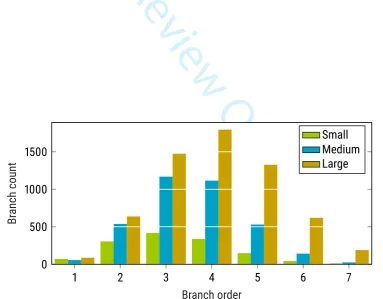
in [18]. The properties of the resulting models are listed in Table 2. Furthermore, the branch count
132
distribution per branch order is visualized in Fig. 2. The count of the branches is important as
133
leaves are placed near the tips of the branches.
134
The small and medium oaks were similar in height, but the latter had about 2.6 times more
135
branches when measured in total count and in length. The large oak had the most branches for
136
all branch orders, and almost twice the volume of the medium oak.
137
2.3
Leaf generation algorithm
138
This section describes an algorithm to populate QSMs with leaves. The main inputs of the
algo-139
rithm are distributions that control the position, orientation, and size of the leaves. These
distribu-140
tions are sampled to retrieve the parameters of individual leaves. The approach can be described
141
as simplified, or na¨ıve, for three reasons: 1) position, orientation and size are sampled
indepen-142
dently, which is to say that,e.g., the size of a leaf may not affect its orientation; 2) simple controls
143
for phyllotaxy and clumping effects are yet to be implemented (although there is some control
144
when generating the petioles); and 3) the only effect leaves have on one another is that they
145
are prevented from intersecting. We call this procedure theFoliage and Needles Na¨ıve Insertion
146
algorithm, or the FaNNI-algorithm in short.
147
2.3.1
Overview of the procedure
148
The inputs of the algorithm are a collection of QSM blocks, leaf basis geometry, target leaf area
149
to be distributed, and petiole and leaf parameter distributions. Details of the roles of the leaf basis
150
geometry and the distributions are presented in Sects. 2.3.2 and 2.3.3, respectively. The process
151
can be viewed as two separate stages: I) generating candidate leaves, II) accepting candidates
152
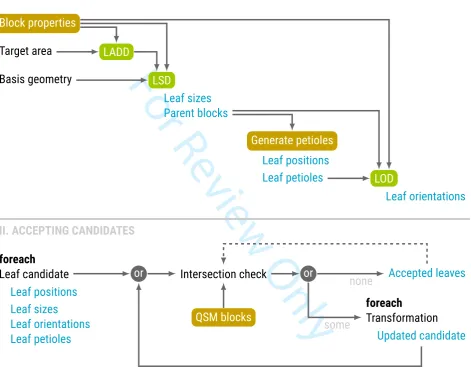
while preventing intersections. An overview of the process is provided in Fig. 3.
153
The first stage begins by distributing the available leaf area onto the blocks. The leaf area
154
density distribution (LADD) determines the relative probability for a block with given parameters to
155
have leaf area. After sampling the distribution with the block properties, each block has a target
156
leaf area, or a leaf area budget, that will be divided into individual leaves by sampling the leaf size
157
distribution (LSD).
158
For the leaf size determination the blocks are processed in random order. To match the target
159
leaf area as closely as possible the cumulative area difference with respect to the target is updated
160
after each leaf. While there is room in the current block, or the cumulative area budget, a new
161
leaf is added to that block. The algorithm assumes that all the generated leaves have the same
162
For Review Only
geometry, and thus we can sample a leaf length value which can be converted to area. After this
163
step, the number of generated leaves and the block parent of each leaf are known.
164
Next, the locations of the leaves are determined by physically attaching them to their branches
165
by the petioles. Because TLS measurements usually cannot capture petioles as they are too small
166
to be detected reliably, all the petioles are generated: The petiole’s starting point, orientation and
167
length are determined by sampling appropriate parameter distributions given by the user. The
168
end point of a petiole also determines the origin of the respective leaf. Although the exact petiole
169
geometry is computed, they are considered insignificant compared to the blocks and the leaves,
170
and thus they are excluded later from the intersection detection process.
171
The final property to sample is the leaf orientation. The leaf orientation distribution (LOD) is
172
used to determine the direction and the surface normal of each leaf. Once this is done, all leaves
173
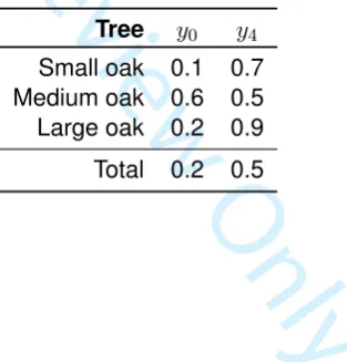
have a fixed position, orientation and scale, and their geometry can be computed by transforming
174
the leaf basis geometry accordingly.
175
At this point it is possible, and even likely with a high leaf count, that some of the leaf candidates
176
intersect one another, or with the blocks, as they were generated independently. However, the
177
goal is to produce a model without leaf intersections, and thus in the second stage the leaves are
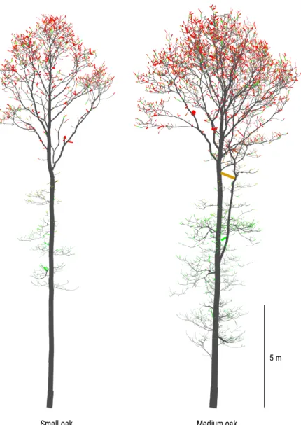
178
checked one-by-one for intersections before adding them to the list of accepted leaves.
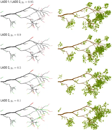
179
If a leaf candidate intersects a block or an accepted leaf, it is possible to try to change the
180
position, orientation and scale of the leaf and check whether the intersection was avoided. If it
181
was, the leaf candidate is accepted, if not, the process can be repeated any number of times with
182
a different transformation applied to the parameters. If despite all the transformations, intersections
183
cannot be avoided the candidate is discarded. An example of how intersection prevention can be
184
implemented in described in Sect. 2.3.4. The leaf generation process stops when all the leaves
185
have been processed, unless some other stopping condition has been given, such as a target leaf
186
area of accepted leaves.
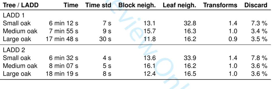
187
2.3.2
Leaf model
188
The leaf model defines the basis geometry of an individual leaf. This geometry is the same for
189
all the sampled leaves, but it is scaled, rotated and translated to receive the final leaf
geome-190
try, during the generation process. Thus all the generated leaves have the same shape but the
191
size and orientation can vary. In the simplest case, the basis geometry can be a single triangle,
192
allowing fast leaf cover generation due to simple intersection detections. For examples of basis
193
geometries consisting of triangles, see Sect. 2.6. On the other hand, there is no upper limit for
194
the complexity of the basis geometry, other than computational time requirements to ensure
non-195
intersecting leaves. Thus, it is possible to represent more complicated shapes, e.g., a leaf with
196
three-dimensional curvature, or a compound-leaf with several leaflets, that do not have to lie on
197
For Review Only
the same plane. However, to simplify the generation process, it is possible to use a simplified basis
198
geometry while generating the leaves, which is then replaced with something more complex, as
199
long as the change does not introduce additional intersections.
200
The origin of the leaf basis coordinate system is assumed to be the point where the petiole
201
connects to the leaf. Leafdirectionis the direction from the origin towards the tip of the leaf, and
202
perpendicular to this lies the leafnormal that defines the direction to which (most of) the leaf area
203
is facing. The length of the basis geometry, i.e. leaf length, is fixed at unity. Other dimensions
204
are given in respect to that. During leaf parameter sampling only the leaf length is sampled as it
205
determines the leaf area when the basis geometry is fixed. Note that it is not required to compute
206
the exact geometry of the leaf candidates before intersection prevention stage.
207
2.3.3
Leaf and petiole parameter distributions
208
Leaf and petiole properties are controlled by multiple user-definable distributions which are
sam-209
pled when leaves are generated. The properties fix the number of leaves, their position, size and
210
orientation. In theory, these distributions are multidimensional as they may depend on any number
211
of block properties, such as height from ground, radius and orientation. They can also be formed
212
as a weighted product or sum of one-dimensional marginal distributions. The purpose of each
213
distribution is described below in the order they are sampled in the implementation.
214
Leaf area density distribution (LADD)
Total leaf area is one of the inputs of the algorithm,215
and leaf area density distribution defines how that area should be distributed to the blocks. Thus,
216
the leaf area density distribution can allocate more leaf area towards the top of the tree and towards
217
the tips of the branches. One could also prevent leaf area being attached directly to stem blocks
218
by using branch order information. Furthermore, the distribution produces a relative mapping of
219
area on the blocks, allowing the distribution to assign any given total area of leaves to the structure
220
model.
221
Leaf size distribution (LSD)
After a leaf area target has been assigned to each block, the222
leaf size distribution is used to sample leaf count and size, so that the target area is matched
223
as closely as possible. This distribution determines the number of leaves to be generated Ninit.
224
However, as no intersections between leaves or between blocks and leaves are tolerated, the final
225
number of leaves may be smaller than initially generated if intersection can not be avoided with
226
transformations,i.e.Nfinal≤Ninitholds.
227
Petiole generation
After size distribution sampling, the number of leaves is known and itbe-228
comes possible to sample the petioles that connect the leaves to their block parents. Similarly to
229
For Review Only
leaves, petiole parameters include the starting point, orientation and length of the petiole, which
230
effectively also determine the starting points, or origins, of the leaves. It would be possible to
231
model the petioles as 3D objects, like small cylinders, but the implementation considers them only
232
as line segments, and they are excluded from the intersection prevention step.
233
Leaf orientation distribution (LOD)
The final distribution controls the orientation of the234
leaves. This distribution controls the directions and normals of the leaves, and can be used to
235
describe,e.g., which parts of the tree areerectophileand which areplanophile.
236
2.3.4
Intersection prevention
237
Sampling the presented leaf and petiole parameter distributions results in a list ofNinit candidate
238
leaves. But because each sample is independent of the rest, the leaves may intersect with other
239
leaves in the list, or blocks of the QSM. To avoid intersections, leaves are only accepted to the final
240
collection of leaves if they do not intersect with other geometry.
241
The accepted leaves list is initialized as empty. One-by-one, the initial leaves are checked, so
242
that they do no intersect with any of the blocks or the accepted leaves. To avoid a low acceptance
243
rate, an intersecting leaf is not discarded instantly. Instead a number of preselected user-defined
244
transformations are applied to the leaf candidate, and intersection checking is repeated. A
trans-245
formation may consist of any combination of scaling, rotation and translation, but they are applied
246
in that order. Only if none of the preselected transformations prevent all the intersections, the
247
candidate is discarded.
248
2.4
Leaf density model
249
Sect. 2.3 described an algorithm to generate exact leaf geometry by sampling certain
distribu-250
tions that depended on individual block parameters. However, in some cases it is not necessary
251
to compute the exact geometry, but rather to view the leaves as an abstract density around the
252
branches [19]. Such an approach saves computational resources as there is no need to compute
253
and store a lot of geometry. This is especially relevant for computations with needles as their
num-254
ber often far exceeds the number of broadleaves for similar sized trees. This abstract approach
255
without exact leaf realizations can be suitable for many applications,e.g., ray tracing operations in
256
radiative transfer and gap fraction computations. However, exact geometry may be better suited
257
for some applications,e.g., requiring realistic visualization, and it is also a more straight-forward
258
way to study effects on a single broadleaf of needle scale.
259
The distributions defined earlier depended on block properties which essentially means, that
260
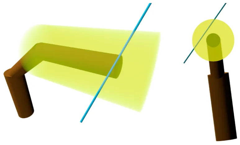
each block defines a density, size and angle distribution around itself. In the case of a cylindrical
261
QSM, this can be viewed as aleaf density cylinder around the block (See Fig. 4). The radius
262
For Review Only
(and length) of the leaf cylinder is defined by petiole length and leaf size distributions. Let us next
263
briefly justify the leaf cylinders as potentially useful and consider ray tracing with leaf cylinders
264
as an example. One possible approach for ray tracing applications would be to determine an
265
absorption rate for the leaf cylinder, which can depend on distance from the cylinder axis, and
266
where the rate can be stochastic (cf. the turbid medium analogy [4]). Branch cylinders can be
267
viewed as infinitely dense, and thus hits occur at their surface. When enough of the energy of a
268
simulated beam is absorbed, a hit occurs inside a leaf cylinder. If the application requires it, an
269
incidence angle can be sampled from the orientation distribution stored in the respective block.
270
2.5
Inserting needles
271
Although this paper focuses on demonstrating broadleaf insertion, it is possible to use the
algo-272
rithm with needles in different ways. The most obvious method is to use a tiny cylinder to represent
273
a single needle and use that as a basis geometry. However, the computational requirements of the
274
insertion would be enormous (but not impossible [20]), as they would be for any further application
275
using the resulting model.
276
A less resource-consuming approach would be a modification of the leaf density cylinder
ap-277
proach described in Sect. 2.4. Rather than inserting needles at all, they could be viewed as a
278
density distribution around the blocks (cf. [19]). Note that the distribution does not have to be
279
uniform, and thus it can be used to account for needle phyllotaxy. Additional buds could also be
280
introduced as density cylinders if the QSM does not contain the level of details in terms of
branch-281
ing structure required by the user. Even though exact needle geometry is not generated, it is
282
important to incorporate the needle phyllotaxy in any ray tracing operations inside needle density
283
cylinders, as it is key in simulations including needles [21].
284
A third option would be to use a needle bud as the basis geometry. An example needle bud
285
suitable for visualization applications can be seen in Fig. 5. Even though the model is complex, it
286
can be simplified to a cylinder during the intersection checking stage. The complex model can still
287
be used for visualizations, or in further computations when required.
288
2.6
A M
ATLABimplementation
289
The leaf insertion algorithm was implemented in MATLAB [22]. The supporting classes and the
290
main function of the implementation are presented below. Currently the implementation works
291
with leaves, where the basis geometry is a collection of triangles, and cylindrical QSMs, but the
292
structure of the implementation is modular, so that it is easy to extend to other types of leaves and
293
blocks as necessary.
294
For Review Only
2.6.1
Classes
295
The following classes were written to make the implementation as modular as possible. Especially,
296
theLeafModelandQSMBabstract classes were designed to define interfaces for easy extendibility
297
when using other structures than cylindrical QSMs, or triangle-based leaf models.
298
LeafModel
The objects of this class have two main purposes in terms of the data they hold.299
First they contain the leaf basis geometry, that is transformed to determine the geometry of
gen-300
erated leaves. Secondly, they hold the parameters of the accepted leaves,i.e., leaf origin, scale,
301
direction and normal. In terms of functionality the class is responsible for defining an intersection
302
detection method for two leaves. There is also a method for converting the geometry of a leaf into
303
a collection of triangles. Thetrianglesmethod is required mainly when detecting intersections
304
between a leaf and a block.1There is also a method for adding a new, accepted leaf to the model.
305
LeafModel is an abstract class, used only for defining the required interface for subclasses
306
rather than actually creating instances. This allows the class to be extended by creating
sub-307
classes, such as, the implementedLeafModelTriangleclass for leaf models, where the leaf
ba-308
sis geometry consists of vertices and triangular faces. This class already allows numerous leaf
309
shapes, as seen in Fig. 6, but the user can extend the possibilities by implementing a subclass of
310
LeafModel,e.g., for leaf geometry defined with B ´ezier curves, or other vertex–face based
geome-311
tries but with more optimized intersection detection than checking each triangle separately.
312
QSMB
The class name is an acronym for Quantitative Structure Model Blocks, and itessen-313
tially acts as a container for QSM block information. The class is abstract and used to define an
314
interface for its subclasses. The interface includes a method for reading block properties, such
315
as position, orientation and branch order, and to detect intersection between blocks and triangles.
316
Furthermore, aQSMBobject is responsible for generating the petioles of the leaves using the block
317
geometry. Finally, there is a method for converting the blocks of a QSM into aCubeVoxelization
318
object, which is used to optimize intersection detection.
319
As an example subclass, theQSMBCylindricalwas created to contain cylindrical QSM data. In
320
this class the block data consist of cylinder parameters for the geometry, and branching topology,
321
such as, branch order information. The user can extend the implementation to work on other types
322
of structure models, by providing the appropriate subclass definition.
323
The QSMBCylindricalclass also defines default uniform distributions for the petiole
param-324
eters. In this initial implementation the petiole parameters are the following, with the lower and
325
upper limits in parenthesis: relative position along cylinder axis (0,1); relative position in radial
326
direction when connected to the end circle of the last cylinder in a branch (0,1); rotation around
327 1
Otherwise you would have to write a separate intersection detection function for each leaf and block type pair.
For Review Only
cylinder axis (−π, π); petiole elevation (−π2,π2); petiole azimuth (−π2,π2); and petiole length (2 cm,
328
5 cm).
329
CubeVoxelization
An object of this class is a voxelization of a fixed 3D space into cubical330
voxels with a fixed edge length. ACubeVoxelizationobject has a minimum and a maximum point
331
and the space between them is divided into a finite number of cells. Object references can be
332
stored into the cells to indicate that the objects occupy at least a part of that voxel. In the main
333
function of the leaf insertion implementation, voxelizations are used to store and find candidate
334
leaves and blocks, to perform more accurate intersection detection. Furthermore, the edge length
335
of the voxelizations is set as the maximum leaf size produced by sampling the leaf size distribution
336
function.
337
2.6.2
Main function
338
qsm_fanniis the main function that receives the QSM as aQSMBobject, an initializedLeafModel
339
object that contains the leaf basis geometry, and total leaf area to be distributed. The leaf area
340
parameter can have two components; one for the initial leaf areaAinitto be generated, and one for
341
the target leaf areaAtarget≤Ainit. This can be used to increase the probability that the target area
342
is reached, even if some of the generated leaves are discarded due to unavoidable intersections.
343
There are also numerous optional inputs for the user to customize, such as the distribution
344
functions and transformations during the intersection prevention step. However, default options
345
are available for all the remaining parameters.
346
The main output of the function is aLeafModelobject derived from the corresponding input,
347
but it now contains the accepted leaves, petiole start points, and a vector of parent block indices
348
of each accepted leaf.
349
2.6.3
Default leaf parameter distributions
350
The implementation contains default distribution functions for leaf parameter properties, and they
351
are described below. At the moment these defaults are not designed to be biologically accurate,
352
but rather just to provide an example of distributions. However, there are plans to improve the
353
realism and usability of the default options in future versions, by offering the user a choice between
354
common options, such as a spherical distribution for the leaf orientation.
355
Leaf area density distribution
By default the available leaf area is distributed equally to all356
the last cylinders in the branches of the QSM. All other cylinders remain leafless.
357
For Review Only
Leaf orientation distribution
The default LOD is such that most of the leaf area facesup-358
wards, but there is some random variation. The LOD computes an initial leaf normal estimate as
359
a cross product of the petiole direction and a side directions on a horizontal plane. If the initial
360
direction differs less than 20◦ from a reference direction (straight up in this case), then the final
361
normal direction is the reference direction. Otherwise, the final normal is the initial direction rotated
362
towards the reference direction by 20◦.
363
Leaf size distribution
The default LSD samples a leaf length value from a uniform distribution364
with given limits. That value is then scaled with a value based on the relative height of the parent
365
block to ensure that leaves are a little bit larger at the top of the tree.
366
3
Results
367
3.1
Leaf geometry complexity test
368
TheLeafModelTriangleclass enables the use of leaf basis geometries with an arbitrary number
369
of triangles. However, the detection of intersections between leaves requires checking all those
370
triangles which has an enormous effect on computational time. To study the effect of the number of
371
triangles in the basis geometry, a single cylindrical block (length 1 m, radius 0.25 m) was fitted with
372
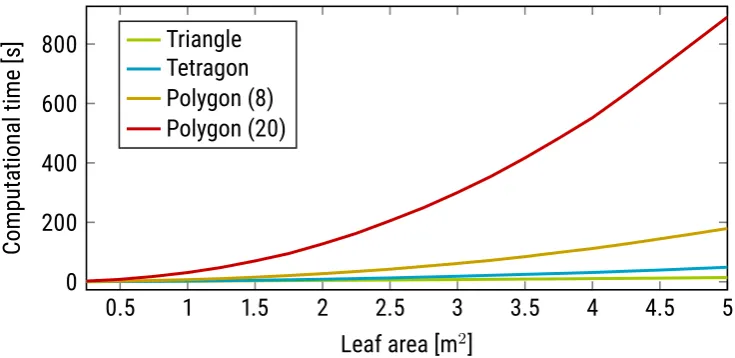
an increasing total area of leaves. The area varied from 0.25 to 5 m2for the four basis geometries
373
in Fig. 6. The process was repeated 10 times for each leaf area–basis geometry pair. The average
374
computational time results are shown in Fig. 7.
375
When using a single triangle, generating non-overlapping leaves was very fast even with the
376
maximum leaf area, 5 m2, taking only 11 s on average. With the two-triangle quadrangle, the times
377
increase 1.8-fold to 4.3-fold in comparison to the single triangle when moving from the lowest to
378
the highest leaf area. For the polygon with 8 triangles, the required time was 8.1-fold already at
379
1 m2and 16-fold at the maximum. The respective multipliers for the 20-triangle polygon were 35.9
380
and a 79.7, which translate to 31 and 891 seconds, respectively.
381
3.2
Leaf area density distribution definitions
382
To demonstrate the leaf insertion algorithm, we defined the two following parametrized leaf area
383
density distributions. While we tested other distributions and parametrizations, these two were
384
chosen because of the low parameter count and overall simplicity.
385
LADD 1 initialized the last 5 % of each branch to have equal portion of leaves, then scaling these
386
proportions with a factor dependent on the relative height of the respective cylinder. The
387
For Review Only
factor had a value of the parametery0at ground level and 1 at the top of the tree. Values in
388
between were interpolated linearly.
389
LADD 2 had an additional parameter to define a cut-off point along a branch. The branch did not
390
have any leaves before this point, which was dependent on the branch order. For the stem
391
the cut-off was at 95 %. For branch orders 4 and above, the cut-off was aty4, and for lower
392
branch orders the cut-off was interpolated linearly. For cylinders after the cut-off point, the
393
probability of leaves was interpolated linearly between zero at the cut-off and one at the tip
394
of the branch. Furthermore, the probabilities were scaled with a factor depending of relative
395
cylinder height as with LADD 1. The scaling factory4 is visualized in Fig. 8 for parameter
396
value 0.4.
397
To find optimal values for the parameters, we performed a simple grid search by varying the
398
values ofy0 andy4 in the closed intervals(0,1)and(0,0.9), respectively. For LADD 1 which only
399
depends on they0parameter, the results are shown in Fig. 9, for LADD 2 the optimal parameter
400
values are listed in Table 3. Optimization was done on the cumulative area difference that was
401
computed as the sum of unsigned leaf area differences in the vertical layers of the trees. The error
402
was normalized with the measured total leaf area of the tree. The total error was computed as a
403
sum over all the trees.
404
For LADD 1 the total optimal value wasy0 = 0.2, which was close to those of the small and
405
large oak trees. However, the optimal value of the medium oak tree was different at 0.7. For LADD
406
2 the total optimum values werey0= 0.2andy4 = 0.5, but there were differences in the optimal
407
parameter values between the individual trees.
408
Fig. 10 visualizes the LADD 2 distribution with the optimal parameter values on the small and
409
medium oak trees. Gray parts have no leaves, green parts have some, and red parts have a lot
410
of leaves. Furthermore, Fig. 11 shows similar LADD heat-maps and corresponding generated
411
leaves. Note that in Fig. 11 LADD 1 is the same as LADD 2 with parameter valuey4= 0.95. Going
412
from top to bottom the regions of high probability of leaves spread from the very tip towards the
413
base of the branch. In the top two rows, the leaves are very concentrated to the tips, whereas in
414
the latter two the leaves are more evenly spread along the high order branches.
415
3.3
Leaf insertion test for oak trees
416
Each of the three oak trees were inserted with their measured leaf area (highlighted in Table
417
1). The two LADDs described above with the optimal parameters were used, and all tree–LADD
418
pairs were repeated ten times. As we lacked reference data for the leaf orientation and leaf size
419
distributions, defaults from the MATLAB implementation were used. To match the measured leaf
420
sizes for each tree, the limits for the default uniform leaf length distribution were derived from the
421
For Review Only
average leaf area measurements. The mean leaf lengthli for treeiwas computed as follows:
422
li= √
Ai
r/2, (1)
whereAiis the average leaf area for treei,r≈0.6is the ratio between the width and length of the
423
leaf basis geometry, which in this case was the quadrangle from Fig. 6 to keep the triangle count
424
low. The leaf length limits were computed for each tree as al±1 cm.
425
The computations were done on a quad-core computer (Intel Core i7-6700K 4GHz, 32 Gb
426
RAM). The computational mean times and standard deviations over the ten repeats are listed in
427
Table 4. The average computational time per QSM block was between 20 and 40 ms for all the
428
trees. Most of the computational time (95.3 %) was spent on detecting intersections, which further
429
supports using the simplest possible leaf basis geometry. The table also lists the average number
430
of required block and leaf neighbour computations, the average number of performed
transfor-431
mations to avoid intersections, and the discarded leaf candidate percentage. The small oak tree
432
had twice the leaf area per branch in comparison to the other two trees, which explains why there
433
were twice as many neighbouring leaf computations and discarded leaves. The results suggest
434
that it would be sufficient to sample 5–10 % more leaves than the target leaf area to account for
435
discarded leaves. The results show that the vast majority of leaf candidates are accepted without
436
any transformation as the average number of tried configurations was between 1.0 and 1.5 for all
437
the trees.
438
Fig. 12 shows a top view of all the oak trees with leaves generated with both LADDs, and Fig.
439
13 shows a side view of the LADD 1 generated leaf covers for the medium and large oaks. The
440
differences between the leaf covers generated with LADD 1 and LADD 2 are subtle, but noticeable.
441
As the higher order branches have a lower cut-off point along the relative position on the branch,
442
leaf cover is more even, making the gap fraction smaller on LADD 2 covers.
443
To compare the generated leaf distributions to the measured data, the leaves were placed in
444
the same vertical bins listed in Sect. 2.1 according to their centre. The signed difference between
445
generated and measured leaf count and area are listed in Table 5. Negative values mean that
446
the tree or layer should have had more leaves or leaf area, positive values are the opposite. Both
447
LADDs were able to match the measured leaf area on tree-level because that was the stopping
448
condition. The tree-level leaf counts are only between 500 and 3500 below the target values.
449
Relative to the total leaf count the differences were 7.5 %, 0.9 % and 2.0 % for the small, medium
450
and large oaks, respectively.
451
The layer-level differences were much higher, which suggests that the vertical distribution
gen-452
erated by the proposed LADDs did not match the measurements. With LADD 2 the top layer of
453
the large oak was missing over 90 m2 of leaf area while the layer below that had an excess of
454
For Review Only
about 60 m2. Results for the small oak were similar, which suggests lowering they
0 parameter.
455
However, the opposite was true for the medium oak, which had about 6 m2of extra leaf area in the
456
upper layer.
457
4
Discussion
458
The above results presented two relatively simple LADD functions that used branch order, relative
459
height and relative position along a branch to determine the portion of leaf area to be assigned to
460
a block. However, the implementation allows for the user to write more complex LADD functions
461
that make use of additional information, such as, absolute height (whether the block is above the
462
surrounding canopies) and absolute orientation (north or south side of the stem). Due to limited
463
reference data only the LADD was optimized. However, if detailed leaf angle or leaf size
measure-464
ments are available, it is possible to optimize the respective distribution in a similar manner.
465
The LADD parameter optimization results and the conflicting layer difference results show that
466
the presented LADDs are not able to capture the differences in the leaf area distributions of the
467
three oaks trees. Further studies should be made to asses whether the underlying leaf
distribu-468
tions differ between these three trees, or whether it is simply a matter of choosing a better LADD.
469
It should also be noted that the manual leaf measurements were limited with only 8 data points in
470
total for the three trees, and as such, more detailed and comprehensive measurements would be
471
beneficial. Some of the leaf area difference can also be explained by uncertainties in estimating
472
leaf area and count for the vertical layers, and by missing branches in the upper canopy in the
473
QSMs.
474
The parameters of the two LADDs were optimized by using a grid search where exact leaf
475
geometry was generated at each grid position. This made the optimization computationally
inten-476
sive as 95 % of the computational time was spent on intersection prevention, which forced a low
477
parameter count. However, in retrospect it was unnecessary to generate leaf geometry, because
478
as the results showed the discard rate was very low, which means that the LADD of the output
479
was very close to the input. Thus, optimization according to,e.g., vertical layers can be simplified
480
to only include distributing the available leaf area onto the structure model and exclude both leaf
481
size and orientation sampling and especially the computation of exact geometry.
482
Future research should also include testing the importance of the intersection prevention for
483
various applications, i.e., whether possibly intersecting and non-intersecting leaves differ
signif-484
icantly in terms of required resources and produced level of detail. This way we would know
485
whether it is sensible to perform the intersection prevention step, e.g., for simulations studying
486
light use efficiency.
487
In this paper, the proposed method was only used to generate leaf covers according to
user-488
For Review Only
given distributions. However, also interesting would be to see if this algorithm could be used
489
to invert or approximate the real-leaf distributions of a given tree, with simple non-destructive
490
and non-direct measurements. For example, it would be possible to test whether gap-fraction
491
measurements and suitable parametrizations of the leaf distributions can be used to optimize the
492
distribution parameters, to derive a mathematical or even a biological explanation for the real leaf
493
distribution. With the method, it is possible make such simulations and study this inverse problem.
494
It should be noted, that such inversion does not reconstruct exact leaf geometry but rather gives an
495
approximation of their distributions. Such an approach could produce new understanding of what
496
affects the distribution of leaves for a specific tree. Furthermore, it would allow the generation of
497
leaf covers that follow the reconstructed distribution for the same tree or some other tree.
498
Currently the algorithm views each leaf independent from the others (apart from intersection
499
prevention), which is one of the reasons for calling the algorithm na¨ıve. However, in most tree
500
species leaves follow a certain phyllotaxy or the leaves are clumped together,e.g., their petioles
501
originate near one another, or even from the very same spot [23]. We are planning to implement
502
simple phyllotaxy controls in future versions of the FaNNI implementation. The level of clumping
503
could be defined as a separate distribution, that would be used to sample the size of a clump and
504
variation in petiole and leaf parameters for the leaves within the clump.
505
In nature leaves are often connected to branches that are small in diameter. Because of the
506
limitations of the TLS technology, such branches are often poorly sampled in the resulting point
507
clouds. Therefore, they can be excluded from the reconstructed QSM also, which means that
508
when leaves are inserted, they are connected to branches that are too large. To counter this
509
shortcoming, it is possible to perform a pre-processing step that inserts small branches to the
510
structure model, which will be given a high probability of leaves when defining the LADD function.
511
Although the implementation enables the use of leaf basis geometries consisting of any number
512
of triangles, the results show that additional complexity multiplies the expected computational
513
time by large factors. However, if detailed leaf geometry is required for later computations, it
514
is possible to use a simplified stand-in basis geometry that encapsulates the complex shape to
515
prevent overlapping during generation, and replace the geometry afterwards. Such a procedure
516
could even be build-in to an extension of theLeafModelclass.
517
5
Conclusion
518
We have presented an algorithm to generate non-intersecting leaves to a QSM, that follow
user-519
defined position, size and orientation distributions. A MATLABimplementation of the algorithm was
520
also presented. Currently, the implementation allows the use of any leaf shape consisting of an
521
arbitrary number of triangles.
522
For Review Only
In order to present leaf property distributions in a compact yet versatile format, we propose a
523
scheme where a QSM is divided into blocks that determine, and can be used to contain, property
524
information for leaves that are to be connected to it. This means that we can assign the available
525
leaf area, leaf size and orientation parameters to the blocks of a QSM even without generating
526
leaves. Then we can do one of the following:
527
• Visualize the property distributions by colouring the blocks according to their respective
prop-528
erty values as seen in the case of leaf area density distributions,e.g., in Figs. 10 and 11.
529
• Sample the user-defined distribution with the parameter values and generate exact leaf
ge-530
ometry as was done in Sect. 3.
531
• View the leaves as a probability distribution around the QSM blocks, and rather than
com-532
puting exact leaf geometry do computations by determining a probability of a hit and the
533
incidence angle when a beam enters the vicinity of a block.
534
Although any triangle-based geometry is possible for the leaves, a simple test of adding an
535
increasing area of leaves to a single cylindrical block showed that complex leaf shapes can
dras-536
tically increase the computational time, at least with the current implementation. Thus, the leaf
537
basis geometry should be kept as simple as possible, or optimization is required for intersection
538
detection.
539
To demonstrate leaf generation, we presented two different LADDs and applied them to three
540
oak trees trying to match field measured leaf count and areas. The measurements were done
541
with 2 to 4 vertical bins per tree, and the average leaf area was also recorded for each tree.
542
Simple uniform leaf size distribution (with some scaling based on height) and planophile orientation
543
distribution were used, while the main focus was on optimizing the LADDs. The two suggested
544
LADDs were able to match leaf area and count per tree, but the vertical distribution of leaves had
545
major errors despite the optimization. Further research is required to understand the cause of the
546
leaf area differences.
547
A further goal is to use the leaf-augmented QSM (L-QSM) to incorporate a number of biological
548
principles such as the availability of resources (mass and energy exchanges between vegetation
549
and atmosphere, and phyllotaxy) to construct as self-consistent tree models as possible. One can
550
include stochastic variations in the same sense as in the creation of 4D QSMs [24], extending that
551
scheme to fully functional trees. This approach would enable a large number of applications to
552
verify and refine assumed biological postulates of theoretical models, and then use the resulting
553
full-scale 3D and 4D models for predictions and the modelling of ecological systems at various
554
size and complexity scales, including large-scale statistical (allometric) estimates.
555
For Review Only
Data Accessibility
556
The MATLABimplementation of the FaNNI-algorithm is available on GitHub
557
(https://github.com/InverseTampere/qsm-fanni-matlab). The three oak tree QSMs are
avail-558
able from Eric Casella ([email protected]) upon request, until they are made public,
559
pending the release of an unrelated study.
560
Authors’ contributions
561
Markku ˚Akerblom developed the FaNNI algorithm, wrote the implementation, carried-out the
com-562
putations, and drafted the manuscript. Eric Casella acquired the TLS measurements, computed
563
the QSMs and led the destructive leaf sampling experiment. Mathias Disney, Mark Danson, Rachel
564
Gaulton and Lucy Schofield participated in that experiment. Pasi Raumonen, Mikko Kaasalainen,
565
Eric Casella, Mathias Disney, Mark Danson, Rachel Gaulton and Lucy Schofield helped draft the
566
manuscript. All authors gave final approval for publication.
567
Acknowledgements
568
The following additional people participated in the oak tree leaf measurements: Ian Craig, Steve
569
Coventry, Marc Sayce and David Payne from the Forest Research UK; Andrew Burt, Ross
Haw-570
ton, Jingjing Yan and Meng Yu from the University College London; Ewan Pinnington from the
571
University of Reading; and Amy Danson and Jennifer Danson.
572
This study was funded by the Academy of Finland research project Centre of Excellence in
573
inverse problems[284715], and by the Forestry Commission GB.
574
Competing interests
575
The authors have no competing interests.
576
References
577
[1] Casella E, Sinoquet H. Botanical determinants of foliage clumping and light
in-578
terception in two-year-old coppice poplar canopies: assessment from 3-D plant
579
mock-ups. Annals of Forest Science. 2007;64(4):395–404. Available from:
580
https://doi.org/10.1051/forest:2007016.
581
For Review Only
[2] Newnham GJ, Armston JD, Calders K, Disney MI, Lovell JL, Schaaf CB, et al. Terrestrial Laser
582
Scanning for Plot-Scale Forest Measurement. Current Forestry Reports. 2015;1(4):239–251.
583
Available from:http://dx.doi.org/10.1007/s40725-015-0025-5.
584
[3] Woodgate W, Disney M, Armston JD, Jones SD, Suarez L, Hill MJ, et al. An improved
585
theoretical model of canopy gap probability for Leaf Area Index estimation in woody
586
ecosystems. Forest Ecology and Management. 2015;358:303 – 320. Available from:
587
https://doi.org/10.1016/j.foreco.2015.09.030.
588
[4] Ross J. The radiation regime and architecture of plant stands. Tasks
589
for Vegetation Science. Springer Netherlands; 1981. Available from:
590
http://doi.org/10.1007/978-94-009-8647-3.
591
[5] Raumonen P, Kaasalainen M, ˚Akerblom M, Kaasalainen S, Kaartinen H, Vastaranta M, et al.
592
Fast Automatic Precision Tree Models from Terrestrial Laser Scanner Data. Remote Sensing.
593
2013;5(2):491–520. Available from:http://dx.doi.org/10.3390/rs5020491.
594
[6] Hackenberg J, Spiecker H, Calders K, Disney M, Raumonen P. SimpleTree—An Efficient
595
Open Source Tool to Build Tree Models from TLS Clouds. Forests. 2015;6(11):4245–4294.
596
Available from:http://dx.doi.org/10.3390/f6114245.
597
[7] Grau E, Durrieu S, Fournier R, Gastellu-Etchegorry JP, Yin T. Estimation of 3D
vegeta-598
tion density with Terrestrial Laser Scanning data using voxels. A sensitivity analysis of
influ-599
encing parameters. Remote Sensing of Environment. 2017;191:373 – 388. Available from:
600
http://dx.doi.org/10.1016/j.rse.2017.01.032.
601
[8] Disney M, Boni I, Vicari M, Burt A, Calders K, Lewis S, et al. Weighing trees with lasers:
602
advances, challenges and opportunities. Interface Focus. 2017;This issue.
603
[9] B ´eland M, Baldocchi DD, Widlowski JL, Fournier RA, Verstraete MM. On seeing the wood
604
from the leaves and the role of voxel size in determining leaf area distribution of forests with
605
terrestrial LiDAR . Agricultural and Forest Meteorology. 2014;184:82 – 97. Available from:
606
http://dx.doi.org/10.1016/j.agrformet.2013.09.005.
607
[10] Ma L, Zheng G, Eitel JUH, Moskal LM, He W, Huang H. Improved Salient
Feature-608
Based Approach for Automatically Separating Photosynthetic and Nonphotosynthetic
Com-609
ponents Within Terrestrial Lidar Point Cloud Data of Forest Canopies. IEEE
Trans-610
actions on Geoscience and Remote Sensing. 2016;54(2):679–696. Available from:
611
http://dx.doi.org/10.1109/TGRS.2015.2459716.
612
For Review Only
[11] Casella E, Sinoquet H. A method for describing the canopy architecture of coppice poplar
613
with allometric relationships. Tree Physiology. 2003;23(17):1153–1170. Available from:
614
http://doi.org/10.1093/treephys/23.17.1153.
615
[12] B ´eland M, Widlowski JL, Fournier RA, C ˆot ´e JF, Verstraete MM. Estimating leaf
616
area distribution in savanna trees from terrestrial LiDAR measurements.
Agri-617
cultural and Forest Meteorology. 2011;151(9):1252 – 1266. Available from:
618
http://dx.doi.org/10.1016/j.agrformet.2011.05.004.
619
[13] Zheng G, Moskal LM. Leaf Orientation Retrieval From Terrestrial Laser Scanning (TLS) Data.
620
IEEE Transactions on Geoscience and Remote Sensing. 2012;50(10):3970–3979. Available
621
from:http://dx.doi.org/10.1109/TGRS.2012.2188533.
622
[14] Bailey BN, Mahaffee WF. Rapid measurement of the three-dimensional distribution
623
of leaf orientation and the leaf angle probability density function using terrestrial
Li-624
DAR scanning. Remote Sensing of Environment. 2017;194:63 – 76. Available from:
625
http://dx.doi.org/10.1016/j.rse.2017.03.011.
626
[15] H ´etroy-Wheeler F, Casella E, Boltcheva D. Segmentation of tree seedling point clouds into
el-627
ementary units. International Journal of Remote Sensing. 2016;37(13):2881–2907. Available
628
from:http://dx.doi.org/10.1080/01431161.2016.1190988.
629
[16] ˚Akerblom M, Raumonen P, Kaasalainen M, Casella E. Analysis of Geometric Primitives
630
in Quantitative Structure Models of Tree Stems. Remote Sensing. 2015;7(4):4581–4603.
631
Available from:http://dx.doi.org/10.3390/rs70404581.
632
[17] Clawges R, Vierling L, Calhoon M, Toomey M. Use of a groundbased scanning
633
LiDAR for estimation of biophysical properties of western larch (Larix occidentalis).
634
International Journal of Remote Sensing. 2007;28(19):4331–4344. Available from:
635
http://dx.doi.org/10.1080/01431160701243460.
636
[18] Calders K, Newnham G, Burt A, Murphy S, Raumonen P, Herold M, et al. Nondestructive
637
estimates of above-ground biomass using terrestrial laser scanning. Methods in Ecology and
638
Evolution. 2015;Available from: http://dx.doi.org/10.1111/2041-210X.12301.
639
[19] Perttunen J, Siev ¨anen R, Nikinmaa E. LIGNUM: a model combining the structure and
640
the functioning of trees. Ecological Modelling. 1998;108(1–3):189 – 198. Available from:
641
https://doi.org/10.1016/S0304-3800(98)00028-3.
642
[20] Disney M, Lewis P, Saich P. 3D modelling of forest canopy structure for remote
sens-643
ing simulations in the optical and microwave domains. Remote Sensing of Environment.
644
2006;100(1):114 – 132. Available from:https://doi.org/10.1016/j.rse.2005.10.003.
645
For Review Only
[21] Cannell MGR, Bowler KC. Phyllotactic arrangements of needles on elongating conifer shoots:
646
a computer simulation. Canadian Journal of Forest Research. 1978;8(1):138–141. Available
647
from:http://dx.doi.org/10.1139/x78-022.
648
[22] ˚Akerblom M. QSM-FaNNI Matlab implementation source code; 2017.
649
https://doi.org/10.5281/zenodo.800496.
650
[23] Niklas KJ. The Role of Phyllotatic Pattern as a” Developmental Constraint” On the
651
Interception of Light by Leaf Surfaces. Evolution. 1988;42(1):1–16. Available from:
652
https://doi.org/10.2307/2409111.
653
[24] Potapov I, J ¨arvenp ¨a ¨a M, ˚Akerblom M, Raumonen P, Kaasalainen M. Data-based stochastic
654
modeling of tree growth and structure formation. Silva Fennica. 2016;50(1). Available from:
655
http://dx.doi.org/10.14214/sf.1413.
656
![Table 2: Oak tree properties computed from reconstructed QSMs.For Review OnlyOak treePropertySmallMediumLargeBranch count133435796161Cylinder count84292353935428DBH [ mm ]298432848Height [ m ]19.119.621.8Order max.989Total length [ m ]59215522516Volume [ l ]70711692098](https://thumb-us.123doks.com/thumbv2/123dok_us/8671359.872609/25.595.185.411.345.546/properties-computed-reconstructed-onlyoak-treepropertysmallmediumlargebranch-cylinder-height-volume.webp)
![Table 5: Difference between oak leaf count and leaf area in total and in vertical layers.For Review OnlyLADD 1LADD 2Tree / Layer∆ Count∆ Area [ m2 ]∆ Count∆ Area [ mSmall oak-3561+0.0-35810.0 – 11.5 m+1707+5.7+100211.5 – 19.6 m-5268-5.7-4583Medium oak-473+0.0-4329.0 m-3339-8.1-28119.0 – 19.9 m+2866+8.1+2379Large oak-2275-0.1-21578.0 m+9507+12.9+107488.0 – 13.0 m+2758+13.1+325413.0 – 18.4 m+15634+58.7+1588318.4 – 22.4 m-30174-84.8-32040](https://thumb-us.123doks.com/thumbv2/123dok_us/8671359.872609/28.595.119.474.318.529/table-difference-vertical-review-onlyladd-count-msmall-medium.webp)