From Zero-shot Learning to Conventional Supervised Classification: Unseen
Visual Data Synthesis
Yang Long
1, Li Liu
2, Ling Shao
2, Fumin Shen
3, Guiguang Ding
4, and Jungong Han
51
Department of Electronic and Electrical Engineering, University of Sheffield, UK
2
School of Computing Science, University of East Anglia, UK
3
Center for Future Media, University of Electronic Science and Technology of China, China
4
School of Software, Tsinghua University, China
5
Department of Computer Science and Digital Technologies, Northumbria University, UK
1
[email protected], {li.liu, ling.shao}@uea.ac.uk, [email protected], [email protected], [email protected]
Abstract
Robust object recognition systems usually rely on pow-erful feature extraction mechanisms from a large number of real images. However, in many realistic applications, collecting sufficient images for ever-growing new classes is unattainable. In this paper, we propose a new Zero-shot learning (ZSL) framework that can synthesise visual fea-tures for unseen classes without acquiring real images. Us-ing the proposed Unseen Visual Data Synthesis (UVDS) al-gorithm, semantic attributes are effectively utilised as an intermediate clue to synthesise unseen visual features at the training stage. Hereafter, ZSL recognition is converted into the conventional supervised problem, i.e. the synthe-sised visual features can be straightforwardly fed to typical classifiers such as SVM. On four benchmark datasets, we demonstrate the benefit of using synthesised unseen data. Extensive experimental results suggest that our proposed approach significantly improve the state-of-the-art results.
1. Introduction
[image:1.612.328.521.331.471.2]Object Recognition is arguably one of the most funda-mental tasks in computer vision field. Most of the conven-tional frameworks,e.g. Deep Neural Networks (DNN) [22], rely on a large number of training samples to build statistical models. However, such a premise is unattainable in many real-world situations. The main reasons can be summarised as follows: 1) Obtaining well-annotated training samples is expensive. Although abundant digital images and videos
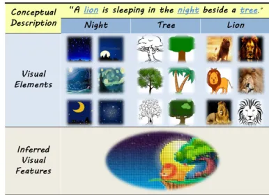
Figure 1. Given a conceptual description, human can imagine the outline of the scene by combining previous seen visual elements. can be retrieved from the Internet, existing search engines crucially depend on user-defined keywords that are often vague and not suitable for learning tasks. 2) The num-ber of newly defined classes is ever-growing. Meanwhile, fine-grained tasks make existing categories go deeper,e.g. to recognise a newly released handbag in a novel pattern. Training a particular model for each of them is infeasible. 3) Collecting instances for rare classes is difficult. For ex-ample, one might wish to detect an ancient or rare species automatically. It could be difficult to provide even a single example for them since available knowledge could be only textual descriptions or some distinctive attributes.
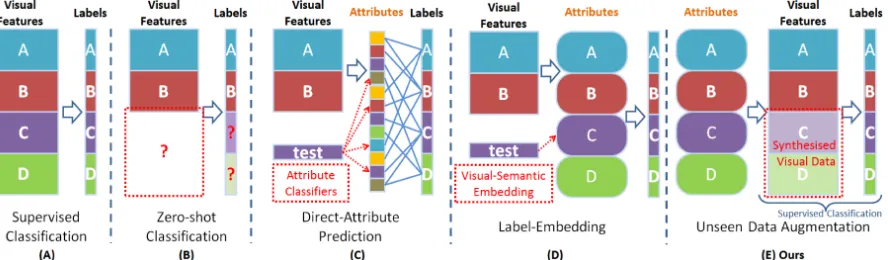
Figure 2. Comparison of supervised and zero-shot classifications and existing ZSL frameworks. (A) a typical supervised classification: the training samples and labels are in pairs; (B) a zero-shot learning problem: without training samples, the classesCandDcannot be predicted; (C) Direct-Attribute Prediction model uses attributes as intermediate clues to associate visual features to class labels; (D) label-embedding: the attributes are concatenated as a semantic embedding; (E) we inversely learn an embedding from the semantic space to visual space and convert the ZSL problem into conventional supervised classification.
can be recognised by only knowing their semantic descrip-tions. However, existing methods cannot expand the train-ing data for new unseen classes. As illustrated in Fig. 2, such frameworks impede existing methods from scaling up since the fixed seen data is eventually limited to represent the ever-growing semantic concepts.
In this paper, we investigate to synthesise high-quality visual features from semantic attributes so that the ZSL problem can be converted into conventional supervised classification. Our idea is inspired by the ability of human imagination, as shown in Fig. 1. Given a semantic de-scription, we human can associate familiar visual elements and then imagine an approximate scene. Accordingly, we synthesise discriminative low-level features from semantic attributes to substitute feature extraction from real images. Our contributions can be summarised as follows:
1) We provide a feasible framework to synthesise un-seen visual features from given semantic attributes with-out acquiring real images. The synthesised data obtained at the training stage can be straightforwardly fed to conven-tional classifiers so that ZSL recognition is skilfully con-verted into the conventional supervised problem and leads to state-of-the-art recognition performance on four bench-mark datasets.
2) We introduce the variance decay problem during semantic-visual embedding and propose a novelDiffusion Regularisationthat can explicitly make information diffuse to each dimension of the synthesised data. We achieve in-formation diffusion by optimising an orthogonal rotation problem. We provide an efficient optimisation strategy to solve this problem together with the structural difference
andtraining biasproblem.
2. Related Work
Zero-shot Recognition Schemes:We summarise previous ZSL schemes in Fig. 2, in contrast to conventional
su-pervised classification (Fig. 2(A)). Since collecting well-labelled visual data for novel classes is expensive, as shown in Fig. 2(B), zero-shot learning techniques [25, 23, 39, 35, 38, 32] are proposed to recognise novel classes without ac-quiring the visual data. Most of the early works are based on the Direct-Attribute Prediction (DAP) model [23]. Such a model utilises semantic attributes as intermediate clues. A test sample is classified by each attribute classifier al-ternately, and the class label is predicted by probabilistic estimation. Admitting the merit of DAP, there are some concerns about its deficiencies. [19] points out that the at-tributes may correlate to each other resulting in significant information redundancy and poor performance. The human labelling involved in attribute annotation may also be unre-liable [18, 50].
To circumvent learning independent attributes, embedding-based ZSL frameworks (Fig.2(C)) are pro-posed to learn a projection that can map the visual features to all of the attributes at once. The class label is then inferred in the semantic space using various measurements [2, 34, 27, 4, 14, 45]. Since the attribute annotations are expansive to acquire, attributes are substituted by the visual similarity and data distribution information in transductive ZSL settings [40, 51, 13, 12, 28, 21, 54, 55, 56]. How-ever, these methods involve the data of unseen classes to learn the model, which to some extent breaches the strict ZSL settings. Recent work [43, 49, 30] combines the embedding-inferring procedure into a unified framework and empirically demonstrates better performance. The closest related work is [7, 8, 31], which takes one-step further to synthesise classifiers or prototypes for unseen classes.
instances rather than mapping visual data to the label space. Semantic Side Information: ZSL tasks require to lever-age side information as intermediate clues. Such frame-works not only broaden the classification settings but also enable various information to aid visual systems. Since textual sources are relatively easy to obtain from the In-ternet, [42, 33] propose to estimate the semantic related-ness of the novel classes from the text. [26, 10, 26] learn pseudo-concepts to associate novel classes using Wikipedia articles. Recently, lexical hierarchies in the ontology engi-neering are also exploited to find the relationships between classes [41, 5, 3].
Although various side information is studied, attribute-based ZSL methods still gain the most popularity. One rea-son is ZSL by learning attributes often gives prominent clas-sification performance [53, 52, 17, 55, 54]. For another rea-son, attribute representation is a compact way that can fur-ther describe an image by concrete words that are human-understandable [11, 29, 15, 1]. Various types of attributes are proposed to enrich applicable tasks and improve the per-formance, such as relative attributes [36], class-similarity attributes [52], and augmented attributes [44]. Our main motivation of this paper not only aims to improve the ZSL performance, but also seeks for a reliable solution for syn-thesising high-quality visual features.
3. Approach
PreliminariesThe training set containscentralised visual features, attributes, and seen class labels that are in 3-tuples:
(x1, a1, y1), ...,(xN, aN, yN)⊆ Xs× As× Ys, whereN
is the number of training samples; Xs = [xnd] ∈ RN×D
is aD-dimensional feature space;As = [anm] ∈ RN×M
is anM-dimensional attribute space; andyn ∈ {1, ..., C}
consists ofCdiscrete class labels. Our framework can cope with eitherclass-levelorimage-levelattributes. For class-level, the instances in the same class share the attributes. GivenNˆ pairs of instances with semantic attributes fromCˆ unseen classes: (ˆa1,yˆ1), ...,(ˆaNˆ,yˆNˆ) ⊆ Au× Yu, where
Yu∩ Ys = ∅,Au = [anm]ˆ ∈ R ˆ
N×M, the goal of
zero-shot learning is to learn a classifier,f : Xu → Yu, where
the samples inXuare completely unavailable during
train-ing. We useCalligraphictypeface to indicate a space. Sub-scriptssandurefer to ‘seen’ and ‘unseen’.hatdenotes the variables that are related to ‘unseen’ samples.
Unseen Visual Data Synthesis: We aim to synthesise the visual features of unseen classes by the given semantic at-tributes. Specifically, we learn an embedding function on the training setf′ :
As → Xs. After that, we are able to
inferXuthrough:Xu=f′(Au).
Zero-shot Recognition: Using the synthesised visual fea-tures, the ZSL recognition is converted to a typical classi-fication problem. It is straightforward to employ
conven-tional supervised classifiers,e.g. SVM, to predict the labels of unseen classesfSVM:Xu→ Yu.
3.1. Unseen Visual Data Synthesis
To synthesise visual features, the most intuitive frame-work is to learn a mapping function from the semantic space to the visual feature space:
min
P L(AsP,Xs) +λΩ(P), (1)
whereP is the projection matrix,Lis a loss function, and
Ω is a regularisation term with its hyper-parameterλ. It is common to choose Ω(P) = kPk2
F, wherek.kF is the
Frobenius norm of a matrix that estimates the Euclidean dis-tance between two matrices. Before the test, we can synthe-sise unseen visual features from the attribute space by given attributes of the unseen instances:
Xu=AuP. (2)
Visual-Semantic Structure Preservation In spite of the simplicity of the above framework, we confront two main problems as follows. 1) Structural difference: in prac-tice, there is often a huge gap between visual and semantic spaces. In pursuance of minimum reconstruction error, the model tends to learn principal components between the two spaces. Consequently, the synthesised data would be not discriminant enough for ZSL purposes. 2) Training bias: the synthesised unseen data can be biased towards the ‘seen’ data and gains a different data distribution to the real unseen data. This problem is due to the regression-based frame-work does not discover the intrinsic geometric structure of the semantic space and cannot capture the unseen-to-seen relationships. Thus, directly mapping from semantic to vi-sual space can lead to inferior performance. We propose to introduce an auxiliary latent-embedding spaceV to recon-cile the semantic space with the visual feature space, where
V = [vnd] ∈ RN×D. In this way, instead of Ω(P), we
can letV preserve the intrinsic data structural information of both visual and semantic spaces:
J =kXs− VQk2F+kV − AsPk2F +λΩ1(V), (3)
where the latent-embedding spaceVis decomposed fromX
andAis then decomposed fromV. Q = [qd′d] ∈ RD×D andP = [pmd] ∈RM×Dare two projection matrices. Ω1 is adual-graphthat is introduced next.
We take theLocal Invariance[6] assumption and solve the problem through a spectralDual-Graphapproach. This is a combination of two supervised graphs that aim to si-multaneously estimate the data structures of bothX andA. The graph of visual spaceWX ∈ RN×N hasN vertices
{g1, ..., gN}that correspond toN data points{x1, ..., xN}
the same number of vertices as N instances of attributes
{a1, ..., aN}. Forimage-level attributes, we constructk-nn
graphs for both visual and semantic spaces,i.e. put an edge between each data pointxn(oran) and each of itsknearest
neighbours. For each pair of the verticesgi andgj in the
weight matrix (not differ inWX andWA), the weight can
be defined as
wij =
1, if giandgjare connected by an edge
0, otherwise.
(4) As a result, we can separately compute the two weight ma-trices WX and WA. It is noteworthy that, for class-level
attributes,WAis computed in a slightly different way.
Ev-ery vertex in the same class is connected by a normalised edge, i.e.wij =k/nc, if and only ifaiandajare from the
same classc, wherencis the size of classc.
In the embedding spaceV, we expect that, ifgiandgjin
both graphs are connected, each pair of embedded points vi andvj are also close to each other. However,
some-times WX andWA are not always consistent due to the
visual-semantic gap. To compromise such conflicts, we compute the mean of the visual and attribute graphs, i.e. W =1
2(WX+WA). The resulted regularisation is:
Ω1(V) =
1 2
N
X
i,j=1
kvi−vjk2wij
=T r(V⊤D
V)−T r(V⊤W
V) =T r(V⊤L
V), (5) whereDis the degree matrix of W,Dii = P
iwij. Lis
known as graph Laplacian matrixL =D−W andT r(.)
computes the trace of a matrix.
Diffusion RegularisationIn this paper, we identify another fundamental problem: variance decay. When we learn vi-sual features from the attributes, in particular when project-ing A toV using P, the dimension difference D ≫ M will lead the learning algorithm to pick the directions with low variances progressively. As shown in Fig. 3, most of the information (variance) is contained in a few projections. As a result, the remaining dimensions of the synthesised data suffers a dramatic variance decay, which indicates the learnt representation is severely redundant. To address the problem, we may expect the concentrated information can effectively diffuse to all of the learnt dimensions through an adjustment rotation [20]. Therefore, we modify the rotating matrixQin Eq. (3). In this paper, we consider an orthog-onal rotation,i.e.QQ⊤ = I, since it is easy to show that T r(Q⊤P⊤
A⊤
AP Q) = T r(P⊤
A⊤
AP)(I is an identity matrix). Such a property is reported in [16] that the orthog-onal rotation can protect the properties captured in the se-mantic space. Next, we show how the rotation can control variance diffusion.
From Eq. (3), the optimal synthesised data isX =VQ,
whereV = AP. We first prove that the overall variance does not change after rotation. Before rotation, V is cen-tralised, i.e. PN
n=1vn = 0. The original overall variance
Γ ofV isΓ = NPD
d=1σd, whereσd = ( PN
n=1v 2
nd)/N
denotes the variance of thed-th dimension. After rotation Q, we have the new variance of each dimensionσ′
dand the
sum of variance of each dimension isΓ′
. We showΓ = Γ′
in the following:
Γ = D X d=1 N X n=1 v2
nd=kVk
2
F =T r(VV ⊤)
= T r(VQQ⊤
V⊤) =
kVQk2
F = D X d=1 N X n=1 x2
nd=N D
X
d=1 σ′
d = Γ ′
. (6)
We hope the overall varianceΓtends to equally diffuse to all of the learnt dimensions in order to recover the real data distribution ofX. In other words, the variance of diffused standard deviations Π in the synthesised data should be small (Π = 1
D
PD
d=1(πd−π¯) 2
, whereπd=pσ′dandπ¯is
the mean of all standard deviations). According to the above Eq. (6), we havePD
d=1π 2
d =
PD
d=1σ
′ d =
PD
d=1σd =ǫ. Next, we show how to minimise Πin our learning frame-work to find the orthogonal rotation:
Π = 1
D D
X
d=1
(πd−¯π)2
= 1 D D X d=1 π2
d+ ¯π
2
−D2
D
X
d=1 πdπ¯
= ǫ
D −
1 D2(
D
X
d=1 πd)2
. (7)
The above equation shows that to minimiseΠis equiv-alent to maximise the sum of diffused standard deviations. Such a deduction is intuitive because our goal is a higher overall sum of standard deviation so that the synthesised data can gain more information. Moreover, we discover a novel relationship between the sum of diffused standard de-viations and the orthogonal rotation:
D
X
d=1 πd =
D X d=1 q σ′ d= D X d=1 v u u t N X n=1 x2 nd/N
= √1
NkX ⊤
k2,1=
1
√
NkQ ⊤
V⊤
k2,1, (8)
wherek.k2,1is theℓ2,1norm of a matrix. According to Eq. (7) and Eq. (8), we can simply maximisekQ⊤
V⊤
(3) and Eq. (5) to form the overall loss function. Such a function aims to minimise the reconstruction error from attributes to visual features, meanwhile preserve the data structure and enable the information to diffuse to all dimen-sions:
min
P,Q,V J =kXs− VQk
2
F+kV − AsPk2F+λT r(V ⊤L
V)
−βkQ⊤
V⊤
k2,1, s.t. QQ⊤=I. (9)
3.2. Optimisation Strategy
The problem raised in Eq. (9) is a non-convex optimi-sation problem. To the best of our knowledge, there is no direct way to find its optimal solution. Similar to [?], in this paper, we propose an iterative scheme by using the al-ternating optimisation to obtain the local optimal solution. Specifically, we initialiseQ= IandV =Xs.The
initiali-sation ofPcan be obtained viaP = (A⊤
sAs)−1A⊤sV. The
whole alternate procedure of the proposed UVDS is listed as follows.
1.V-step:By fixingP andQ, we can reduce Eq. (9) to the following sub-problem:
min
V kXs− VQk
2
F +kV − AsPk2F+λT r(V ⊤L
V)
−βkQ⊤V⊤
k2,1+γk1Vk22, (10)
where the extra termγk1Vk2
2constrains the learntV to be centralised according to Eq. 6. The minimalV can be ob-tained by setting the partial derivative of Eq. (10) to zero and we have
∂J
∂V = 2(VQ− X)Q ⊤
+ 2(V − AP)
+ 2λLV −βVQEQ⊤+γ1⊤1V= 0, (11)
whereE =diag(e1, . . . , ed, . . . , eD)∈ RD×Dand thed
-th element ofE ised = 1/(
√
N πd). By merging the like terms, Eq. (11) can be rewritten as
V(2QQ⊤+ 2αI+βQEQ⊤) + (2λL+γ1⊤
1)V −(XQ⊤+ 2
AP) = 0, (12)
which is a typical Sylvester equation so that V can be efficiently solved by thelyap()function in the MATLAB. Afterwards, the leant V needs to be further centralised: vn ←vn−(P
N
n=1vn)/Nto satisfy Eq. 6.
2. Q-step: By fixingPandV, we can reduce Eq. (9) to the following sub-problem:
min
Q kXs− VQk
2
F−βkQ ⊤
V⊤k2,1, s.t. QQ⊤=I (13)
Since we need to solve Q with the orthogonality con-straint in Eq. (13), in this paper, we adopt the gradient flow
in [47] which is an iterative scheme for optimising generic orthogonal problems with a feasible solution. Specifically, given the orthogonal rotationQtduring thet-th iterative
op-timisation, a better solution ofQt+1 is updated viaCayley
transformation:
Qt+1=HtQt, (14)
whereHtis theCayley transformationmatrix and defined
as
Ht= (I + τ 2Φt)
−1(I
−τ2Φt), (15)
where I is the identity matrix, Φt = ∆tQ⊤
t −Qt∆ ⊤ t is
the skew-symmetric matrix,τ is an approximate minimiser satisfying Armijo-Wolfe conditions [48] and∆is the partial derivative of Eq. (13) with respect toQas
∆t=V⊤
(VQt− Xs)−βV⊤VQtE., (16)
where the diagonal matrixEis defined the same as that in Eq. (11). In this way, for the Q-step, we repeat the above formulation to update Q until achieving convergence.
3. P-step: By fixingQandV, we can reduce Eq. (9) to the following sub-problem:
min
P αkV − AsPk
2
F. (17)
The resulted equation is derived by a standard least squares problem with the following analytical solution:
P = (A⊤ sAs)
−1
A⊤
sV. (18)
In this way, we sequentially updateV,QandPto opti-mise UVDS withT times based on coordinate descent. For each variable, either global or local optimum is achieved and thus the overall objective is lower bounded, which guar-antees the convergence of our method. In practice, UVDS can well converge withT = 5∼10.
3.3. Zero-shot Recognition
Once we obtain the embedding matricesP andQ, the visual features of unseen classes can be easily synthesised from their semantic attributes:
Xu=AuP Q. (19)
It is noticeable that for image-level attributes,Xu
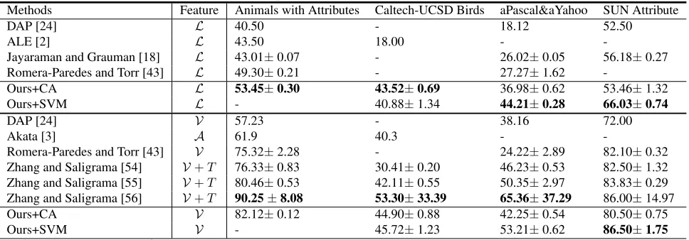
Table 1. Comparison with State-of-the-art methods.
Methods Feature Animals with Attributes Caltech-UCSD Birds aPascal&aYahoo SUN Attribute
DAP [24] L 40.50 - 18.12 52.50
ALE [2] L 43.50 18.00 -
-Jayaraman and Grauman [18] L 43.01±0.07 - 26.02±0.05 56.18±0.27 Romera-Paredes and Torr [43] L 49.30±0.21 - 27.27±1.62
-Ours+CA L 53.45±0.30 43.52±0.69 36.98±0.62 53.46±1.32
Ours+SVM L - 40.88±1.34 44.21±0.28 66.03±0.74
DAP [24] V 57.23 - 38.16 72.00
Akata [3] A 61.9 40.3 -
-Romera-Paredes and Torr [43] V 75.32±2.28 - 24.22±2.89 82.10±0.32 Zhang and Saligrama [54] V+T 76.33±0.83 30.41±0.20 46.23±0.53 82.50±1.32 Zhang and Saligrama [55] V+T 80.46±0.53 42.11±0.55 50.35±2.97 83.83±0.29 Zhang and Saligrama [56] V+T 90.25±8.08 53.30±33.39 65.36±37.29 86.00±14.97 Ours+CA V 82.12±0.12 44.90±0.88 42.25±0.54 80.50±0.75
Ours+SVM V - 45.72±1.23 53.21±0.62 86.50±1.75
L: Low-level feature,A: Deep feature using AlexNet, andV: VGG-19, CA: class-level attributes. T: transductive.
Algorithm 1:Unseen Visual Data Synthesis (UVDS) Input:Training set{Xs, As, Ys},kfork-nn graph
Output:P, QandV
1 InitialiseQ= I,V=XsandP = (A⊤sAs)−
1
A⊤ sV,
whereI∈RD×Dis the identity matrix. 2 Repeat
3 V-Step:FixP,Qand updateVusing Eq. (12). 4 Q-Step:FixP,Vand updateQby following steps:
5 fort= 1 : max iterationsdo
6 Compute the gradient∆tusing Eq. (16);
7 Compute the the skew-symmetric matrixΦt;
8 Compute the Cayley matrixHtusing Eq. (15);
9 Compute theQt+1using Eq. (14);
10 ifconvergence,break; 11 end
12 P-Step:FixV,Qand updatePusing Eq. (18). 13 Untilconvergence
14 ReturnfU V DS(x) =xP Q
4. Experiments
Settings We evaluate our method on four benchmark datasets and strictly follow the published seen/unseen splits. For AwA [23] and aPY [11], we follow the standard 40/10 and 20/12 splits like most of existing methods. For CUB, we follow [2] to use the 150/50 setting. For SUN, we use the simple 707/10 setting as reported in [18, 43, 54]. Meth-ods under different settings [40, 13, 7, 9], or using other var-ious semantic information [36, 52, 1, 3] are not compared with.
Semantic Attributes Existing attributes are divided into image-level and class-level. On CUB, aPY, and SUN datasets, image-level attributes are provided. Our approach can synthesise the visual features for all unseen instances.
We compute class-level attributes by averaging the image-level attributes for each class. For the AwA dataset, only class-level attributes are provided.
Visual FeaturesFor low-level visual features, we use those provided by the four datasets [23, 11, 37, 46]. For deep learning features, we adopt CNN features released by[54] for the four datasets using the VGG-19 model.
Implementation ParametersHalf of the data in each class in the training sets are used as the validation set. We use 10-fold cross-validation to obtain the optimal hyper-parameters λandβ.kis fixed to 10 for thek-nn graph.
4.1. Comparison with the State-of-the-art methods
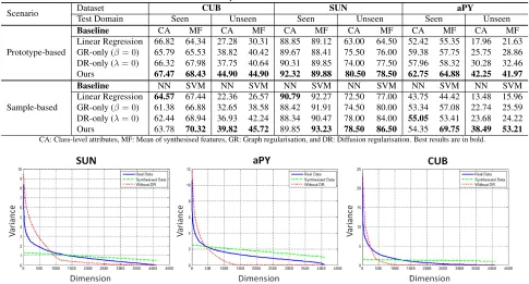
Table 2. Comparison with baseline methods.
Scenario Dataset CUB SUN aPY
Test Domain Seen Unseen Seen Unseen Seen Unseen
Prototype-based
Baseline CA MF CA MF CA MF CA MF CA MF CA MF
Linear Regression 66.82 64.34 27.28 30.31 88.85 89.12 63.00 64.50 52.42 55.35 17.96 21.63 GR-only (β= 0) 65.79 65.53 38.82 40.42 89.67 88.41 75.50 76.00 59.38 57.75 25.75 28.86 DR-only (λ= 0) 66.32 67.98 37.75 40.64 90.31 89.85 74.00 77.50 57.96 58.32 30.28 32.46 Ours 67.47 68.43 44.90 44.90 92.32 89.88 80.50 78.50 62.75 64.88 42.25 41.97
Sample-based
Baseline NN SVM NN SVM NN SVM NN SVM NN SVM NN SVM Linear Regression 64.57 67.44 22.36 26.57 90.79 92.27 72.50 77.00 43.75 44.42 13.48 15.96 GR-only (β= 0) 61.38 66.88 32.65 38.58 88.42 91.91 74.50 80.00 53.34 57.08 22.74 25.59 DR-only (λ= 0) 62.44 68.94 36.93 42.24 88.34 90.47 78.00 84.00 55.05 53.41 23.68 24.22 Ours 63.78 70.32 39.82 45.72 89.85 93.23 78.50 86.50 54.35 69.75 38.49 53.21 CA: Class-level attributes, MF: Mean of synthesised features, GR: Graph regularisation, and DR: Diffusion regularisation. Best results are in bold.
Figure 3. Normalised variances of the synthesised data w.r.t. dimensions. Variance of each dimension is sorted in descending order. We make a comparison between the synthesised data variances ‘with’ (green) and ‘without’ (red) diffusion regularisation. The variances of real data (blue) are computed from real unseen data as references.
performance, our method can also achieve acceptable re-sults with low-level features. In most cases, using SVM can further improve the recognition rates, especially when the class-level attributes are noisy,e.g. on aPY and SUN. How-ever, if the class-level attributes are more precise,e.g. CUB, the class-level NN classifier can be better than SVM.
4.2. Detailed Evaluations
Baseline methodsTo understand the effect of each term in Eq. (9), we compare our method to several baseline meth-ods in Table 2. Since AwA only provides class-level at-tributes, the following experiments are conducted on CUB, SUN, and aPY only. The first method is simplyLinear Re-gressionthat we solve Eq. (1) and synthesise prototypes of unseen classes using Eq. (2). The second and third meth-ods are denoted asGraph-Regularisation (GR) only(β= 0) and Diffusion-Regularisation (DR) only(λ= 0). For the training bias problem, we use the validation set to test the methods on seen classes. We also investigate ZSL under both class-level and image-level attributes scenarios. The first scenario isprototype-based,i.e. each unseen class gains only one visual prototype. We compare two possible ways to obtain the class-level visual prototype: 1) we compute the mean of image-level attributes in each class and use the averaged class-level attributes (CA) to synthesise one visual prototype for each class; 2) we first synthesise the visual features from the image-level attributes and use the
mean of the features (MF) as the class prototype. During the test, we use NN classification to predict the label for the test image. The second scenario issample-based,i.e. each unseen image has one unique attribute description. In this scenario, we fully synthesise all of the visual features of un-seen classes and use them as training examples. We show how an advanced classifier,e.g. SVM, can further boost the performance.
In summary, our method can effectively prevent the training bias whereas the linear regression without regular-isation suffers from 30% performance degradation in aver-age from seen to unseen. DR is complementary to GR and can further boost the performance. There is no significant difference between the CA and MF scenarios. Therefore, our proposed method can be reliably applied to both image-level and class-image-level attributes. Another advantage is that the synthesised visual data can be fed to typical supervised classifiers to achieve better performance, which can be sup-ported by the results using SVM.
con-Figure 4. Success and Failure cases of nearest neighbour matching. The query visual feature is synthesised from its attribute description. We find top-5 nearest neighbours of the query feature from the real instances. It is a match if the nearest instance and the test image have the same label.
centrated in a few dimensions (roughly 1000, 1500, and 500 on SUN, aPY, and CUB) while most of the remaining di-mensions gain very low variances. In comparison, the vari-ances of our proposed synthesised data (green) and real data are more informative. Furthermore, thanks to the DR, the variances in our proposed data are more balanced than real data,i.e. each of the dimension gains the equal amount of information. Such quantitative evidence explains the suc-cess of our proposed method in ZSL recognition.
Finally, we provide some qualitative results of our method. We use the synthesised features as queries and retrieve real images from the unseen datasets. In Fig. 4, we show some success cases that most of the top-5 results are with the same class labels. Particularly, the third result of Bagis the same paired image of the attributes that are used to synthesise the data. Such results demonstrate that the synthesised data is close to the samples from the same class in the feature space. On the contrary, we also provide some failure cases that the top-1 retrieval result is not with the same class label. Some of them are due to the ambiguity of the semantic meaning,e.g. theflea markethas many sim-ilar attributes to theshoe shop. Some other cases,e.g. the
CUB dataset, the real data of the birds are not distinctive to the other classes. Therefore, the NN-based retrieval gives a mixture of true-positives and false-positives. Such failures due to the ambiguity of the visual feature are not common cases. We can still achieve 45.72% overall recognition rate on the CUB dataset.
5. Conclusion
[image:8.612.75.522.82.400.2]References
[1] Z. Akata, M. Malinowski, M. Fritz, and B. Schiele. Multi-cue zero-shot learning with strong supervision. In CVPR, 2016.
[2] Z. Akata, F. Perronnin, Z. Harchaoui, and C. Schmid. Label-embedding for attribute-based classification. InCVPR, 2013. [3] Z. Akata, S. Reed, D. Walter, H. Lee, and B. Schiele. Eval-uation of output embeddings for fine-grained image classifi-cation. InCVPR, 2015.
[4] Z. Al-Halah, T. Gehrig, and R. Stiefelhagen. Learning se-mantic attributes via a common latent space. InVISAPP, 2014.
[5] Z. Al-Halah and R. Stiefelhagen. How to transfer? zero-shot object recognition via hierarchical transfer of semantic attributes. InWACV, 2015.
[6] D. Cai, X. He, J. Han, and T. S. Huang. Graph regularized nonnegative matrix factorization for data representation. Pat-tern Analysis and Machine Intelligence, IEEE Transactions on, 33(8):1548–1560, 2011.
[7] S. Changpinyo, W.-L. Chao, B. Gong, and F. Sha. Synthe-sized classifiers for zero-shot learning. InCVPR, 2016. [8] S. Changpinyo, W.-L. Chao, and F. Sha. Predicting visual
exemplars of unseen classes for zero-shot learning. arXiv preprint arXiv:1605.08151, 2016.
[9] W.-L. Chao, S. Changpinyo, B. Gong, and F. Sha. An em-pirical study and analysis of generalized zero-shot learn-ing for object recognition in the wild. arXiv preprint arXiv:1605.04253, 2016.
[10] M. Elhoseiny, B. Saleh, and A. Elgammal. Write a classi-fier: Zero-shot learning using purely textual descriptions. In
CVPR, 2013.
[11] A. Farhadi, I. Endres, D. Hoiem, and D. Forsyth. Describing objects by their attributes. InCVPR, 2009.
[12] Y. Fu, T. M. Hospedales, T. Xiang, Z. Fu, and S. Gong. Transductive multi-view embedding for zero-shot recogni-tion and annotarecogni-tion. InECCV. 2014.
[13] Y. Fu, T. M. Hospedales, T. Xiang, and S. Gong. Trans-ductive multi-view zero-shot learning. Pattern Analysis and Machine Intelligence, IEEE Transactions on, 37(11):2332– 2345, 2015.
[14] Z. Fu, T. Xiang, E. Kodirov, and S. Gong. Zero-shot object recognition by semantic manifold distance. InCVPR, 2015. [15] C. Gan, M. Lin, Y. Yang, G. de Melo, and A. G. Haupt-mann. Concepts not alone: Exploring pairwise relationships for zero-shot video activity recognition. InAAAI, 2016. [16] Y. Gong and S. Lazebnik. Iterative quantization: A
pro-crustean approach to learning binary codes. InCVPR, 2011. [17] S. Huang, M. Elhoseiny, A. Elgammal, and D. Yang. Learn-ing hypergraph-regularized attribute predictors. In CVPR, 2015.
[18] D. Jayaraman and K. Grauman. Zero-shot recognition with unreliable attributes. InNIPS, 2014.
[19] D. Jayaraman, F. Sha, and K. Grauman. Decorrelating se-mantic visual attributes by resisting the urge to share. In
CVPR, 2014.
[20] H. J´egou, M. Douze, C. Schmid, and P. P´erez. Aggregating local descriptors into a compact image representation. In
CVPR, 2010.
[21] E. Kodirov, T. Xiang, Z. Fu, and S. Gong. Unsupervised domain adaptation for zero-shot learning. InICCV, 2015. [22] A. Krizhevsky, I. Sutskever, and G. E. Hinton. Imagenet
classification with deep convolutional neural networks. In
NIPS, 2012.
[23] C. H. Lampert, H. Nickisch, and S. Harmeling. Learning to detect unseen object classes by between-class attribute trans-fer. InCVPR, 2009.
[24] C. H. Lampert, H. Nickisch, and S. Harmeling. Attribute-based classification for zero-shot visual object categoriza-tion. Pattern Analysis and Machine Intelligence, IEEE Transactions on, 36(3):453–465, 2014.
[25] H. Larochelle, D. Erhan, and Y. Bengio. Zero-data learning of new tasks. InAAAI, 2008.
[26] J. Lei Ba, K. Swersky, S. Fidler, et al. Predicting deep zero-shot convolutional neural networks using textual descrip-tions. InICCV, 2015.
[27] X. Li and Y. Guo. Max-margin zero-shot learning for multi-class multi-classification. InAISTATS, 2015.
[28] X. Li, Y. Guo, and D. Schuurmans. Semi-supervised zero-shot classification with label representation learning. In
ICCV, 2015.
[29] K. Liang, H. Chang, S. Shan, and X. Chen. A unified multi-plicative framework for attribute learning. InICCV, 2015. [30] Y. Long, L. Liu, and L. Shao. Attribute embedding with
visual-semantic ambiguity removal for zero-shot learning. In
BMVC, 2016.
[31] Y. Long, L. Liu, and L. Shao. Towards fine-grained open zero-shot learning: Inferring unseen visual features from at-tributes. InWACV, 2017.
[32] Y. Long and L. Shao. Describing unseen classes by exem-plars: Zero-shot learning using grouped simile ensemble. In
WACV, 2017.
[33] T. Mensink, E. Gavves, and C. Snoek. Costa: Co-occurrence statistics for zero-shot classification. InCVPR, 2014. [34] T. Mensink, J. Verbeek, F. Perronnin, and G. Csurka. Metric
learning for large scale image classification: Generalizing to new classes at near-zero cost. InECCV. 2012.
[35] M. Palatucci, D. Pomerleau, G. E. Hinton, and T. M. Mitchell. Zero-shot learning with semantic output codes. In
NIPS, 2009.
[36] D. Parikh and K. Grauman. Relative attributes. InICCV, 2011.
[37] G. Patterson, C. Xu, H. Su, and J. Hays. The sun attribute database: Beyond categories for deeper scene understanding.
International Journal of Computer Vision, 108(1-2):59–81, 2014.
[38] J. Qin, L. Liu, L. Shao, F. Shen, B. Ni, J. Chen, and Y. Wang. Zero-shot action recognition with error-correcting output codes. InCVPR, 2017.
[40] M. Rohrbach, S. Ebert, and B. Schiele. Transfer learning in a transductive setting. InNIPS, 2013.
[41] M. Rohrbach, M. Stark, and B. Schiele. Evaluating knowl-edge transfer and zero-shot learning in a large-scale setting. InCVPR, 2011.
[42] M. Rohrbach, M. Stark, G. Szarvas, I. Gurevych, and B. Schiele. What helps where–and why? semantic relat-edness for knowledge transfer. InCVPR, 2010.
[43] B. Romera-Paredes and P. Torr. An embarrassingly simple approach to zero-shot learning. InICML, 2015.
[44] V. Sharmanska, N. Quadrianto, and C. H. Lampert. Aug-mented attribute representations. InECCV. 2012.
[45] R. Socher, M. Ganjoo, C. D. Manning, and A. Ng. Zero-shot learning through cross-modal transfer. InNIPS, 2013. [46] C. Wah, S. Branson, P. Welinder, P. Perona, and S.
Be-longie. The caltech-ucsd birds-200-2011 dataset. Technical Report CNS-TR-2011-001, California Institute of Technol-ogy, 2011.
[47] Z. Wen and W. Yin. A feasible method for optimization with orthogonality constraints.Mathematical Programming, 142(1-2):397–434, 2013.
[48] S. Wright and J. Nocedal. Numerical optimization.Springer Science, 35:67–68, 1999.
[49] Y. Xian, Z. Akata, G. Sharma, Q. Nguyen, M. Hein, and B. Schiele. Latent embeddings for zero-shot classification. InCVPR, 2016.
[50] X. Xu, F. Shen, Y. Yang, D. Zhang, T. Shen, and J. Song. Ma-trix tri-factorization with manifold regularizations for zero-shot learning. InCVPR, 2017.
[51] Y. Yang and T. M. Hospedales. A unified perspective on multi-domain and multi-task learning.ICLR, 2015. [52] F. Yu, L. Cao, R. Feris, J. Smith, and S.-F. Chang.
Design-ing category-level attributes for discriminative visual recog-nition. InCVPR, 2013.
[53] X. Yu and Y. Aloimonos. Attribute-based transfer learning for object categorization with zero/one training example. In
ECCV. 2010.
[54] Z. Zhang and V. Saligrama. Zero-shot learning via semantic similarity embedding. InICCV, 2015.
[55] Z. Zhang and V. Saligrama. Zero-shot learning via joint la-tent similarity embedding. InCVPR, 2016.