warwick.ac.uk/lib-publications
Original citation:
Touloupou, Panayiota, Alzahrani, Naif, Neal, Peter, Spencer, Simon E. F. and McKinley,
Trevelyan J.. (2017) Efficient model comparison techniques for models requiring large scale
data augmentation. Bayesian Analysis.
Permanent WRAP URL:
http://wrap.warwick.ac.uk/87993
Copyright and reuse:
The Warwick Research Archive Portal (WRAP) makes this work of researchers of the
University of Warwick available open access under the following conditions.
This article is made available under the Creative Commons Attribution 4.0 International
license (CC BY 4.0) and may be reused according to the conditions of the license. For more
details see:
http://creativecommons.org/licenses/by/4.0/
A note on versions:
The version presented in WRAP is the published version, or, version of record, and may be
cited as it appears here.
Efficient Model Comparison Techniques
for Models Requiring Large Scale Data
Augmentation
Panayiota Touloupou∗, Naif Alzahrani†, Peter Neal‡, Simon E. F. Spencer§, and Trevelyan J. McKinley¶
Abstract. Selecting between competing statistical models is a challenging prob-lem especially when the competing models are non-nested. In this paper we offer a simple solution by devising an algorithm which combines MCMC and importance sampling to obtain computationally efficient estimates of the marginal likelihood which can then be used to compare the models. The algorithm is successfully ap-plied to a longitudinal epidemic data set, where calculating the marginal likelihood is made more challenging by the presence of large amounts of missing data. In this context, our importance sampling approach is shown to outperform existing methods for computing the marginal likelihood.
Keywords:epidemics, marginal likelihood, model evidence, model selection.
1
Introduction
The central pillar of Bayesian statistics is Bayes’ Theorem. That is, given a parameteric model M with parameters θ = (θ1, . . . , θd) and data x = (x1, x2, . . . , xn), the joint distribution of (θ,x) satisfies
π(θ|x)π(x) =π(x|θ)π(θ). (1)
The four terms in (1) are the posterior distribution π(θ|x), the marginal likelihood or evidenceπ(x), the likelihoodπ(x|θ) and the prior distributionπ(θ). The terms on the right hand side of (1) are usually easier to derive than those on the left hand side. The statistician has considerable control over the prior distribution and this can be chosen pragmatically to reflect prior beliefs and to be mathematically tractable. For many sta-tistical problems the likelihood can easily be derived. However, the quantity of primary interest is usually the posterior distribution. Rearranging (1) it is straightforward to obtain an expression for π(θ|x) so long as the marginal likelihood can be computed. This involves computing
∗Department of Statistics, University of Warwick, Coventry, CV4 7AL, UK
†Department of Mathematics and Statistics, Lancaster University, Lancaster, LA1 4YF, UK ‡Department of Mathematics and Statistics, Lancaster University, Lancaster, LA1 4YF, UK,
§Department of Statistics, University of Warwick, Coventry, CV4 7AL, UK
¶College of Engineering, Mathematics and Physical Sciences, University of Exeter, Penryn Campus, Penryn, Cornwall, TR10 9EZ, UK
c
π(x) =
π(x|θ)π(θ)dθ, (2)
which is only possible analytically for a relatively small set of simple models.
A key solution to being unable to obtain an analytical expression for the posterior dis-tribution is to obtain samples from the posterior disdis-tribution using Markov chain Monte Carlo (MCMC; Metropolis et al.,1953; Hastings,1970). A major strength of MCMC is that it circumvents the need to computeπ(x) and this has led to its widespread use in Bayesian statistics over the last 25 years or so. However, Bayesian model choice typically requires the computation of Bayes Factors (Kass and Raftery,1995) or posterior model probabilities, which are both functions of the marginal likelihoods for the competing models. In Chib (1995) a simple rewriting of (1) was exploited to obtain estimates of the marginal likelihood using output from a Gibbs sampler. This has been extended in Chib and Jeliazkov (2001) and Chen (2005) to be used with the general Metropolis-Hastings algorithm. Importance sampling approaches to estimating the marginal likeli-hood have also been suggested (Gelfand and Dey,1994), along with generalisations such as bridge sampling (Meng and Wong,1996), which ‘bridges’ information from posterior and importance samples. More recently approaches have exploited the ‘thermodynamic integral’ such as power posterior methods Friel and Pettitt (2008). Alternative methods such as Sequential Monte Carlo (e.g. Zhou et al., 2015) and nested sampling (Skilling,
2004) do not require any MCMC: computation of the marginal likelihood and samples from the posterior distribution are produced simultaneously. A potential drawback for many of the above approaches to marginal likelihood estimation is that it may not be obvious how to apply them efficiently to models incorporating large amounts of missing data.
It should be noted that there are model comparison techniques such as reversible jump (RJ)MCMC (Green,1995) which can used to compare models without the need to compute the marginal likelihood. RJMCMC works well for nested models where it is straightforward to define a good transition rule for models with different parameters. However, in the case where we have large amounts of missing data it is often necessary to use some form of data augmentation technique, where the missing information is inferred alongside the other parameters of the model. Using RJMCMC becomes much harder in these cases since the dimension of the parameter space (including the augmented data) becomes large. This is exacerbated further when the missing information between the competing models has a different structure. In this latter case the use of intermediary (bridging) models (Karagiannis and Andrieu, 2013) to move between the models of interest is a possibility.
tremendously in devising an efficient estimator of the marginal likelihood. In Section4
we consider final outcome household epidemic data where in the special case of the Reed-Frost model exact, but expensive, computation of the marginal likelihood is possible for comparison purposes. In Section 5we apply the methodology to an epidemic example, for the transmission ofStreptococcus pneumoniae(Melegaro et al.,2004) comparing our algorithm to existing methods for computing the marginal likelihood demonstrating its simplicity and effectiveness in the presence of missing data. Finally in Section 6 we briefly discuss extensions and limitations of the algorithm.
2
Algorithm
Our starting point in the estimation ofπ(x) is to note that we can rewrite (2) as
π(x) =
θ
π(x|θ)π(θ)
q(θ)q(θ)dθ, (3)
where q(θ) denotes a d-dimensional probability density function. We assume that if π(θ)>0 thenq(θ)>0. Then an unbiased estimator,Pqofπ(x) is obtained by sampling
θ1,θ2, . . . ,θN from q(θ) and setting
Pq = 1 N
N
i=1
π(x|θi)
π(θi)
q(θi)
. (4)
Thus Pq is an importance sampled (see, for example, Ripley, 1987) estimate of π(x), and the effectiveness of the estimator given by (4) depends upon the variability of π(x|θ)π(θ)/q(θ).
The remainder of the paper and this Section, in particular, is focussed on how we can effectively exploit (4) in the estimation of π(x). The first observation is that the optimal choice of q(θ) isπ(θ|x), the posterior density but if we knew this, then π(x) would also be known. A simple solution is to use output from an MCMC algorithm to inform the proposal distribution (Clyde et al., 2007). For most statistical models the likelihood times the prior is unimodal for sufficiently large n. In these circumstances, the posterior distribution of θ is almost always approximately Gaussian with mean θ, the posterior mode, and covariance matrix Σ =−I(θ)−1, whereI(θ) denotes the Fisher information evaluated at θ. That is, we have a central limit theorem type behaviour similar to that observed for maximum likelihood estimators asn→ ∞. This central limit theorem approximation is implicitly behind the Laplace approximations of integrals used in Tierney and Kadane (1986), (2.2) and Gelfand and Dey (1994), (8). This underpins the simple suggestion in Clyde et al. (2007) of using a multivariatet-distribution as an importance sampling distribution with location and scale parameters estimated from MCMC output. Alternatively, we can use a “defense mixture” (Hesterberg,1995),
p is a mixing proportion. This proposal ensures that the ratio of the prior density to the proposal density is bounded above by 1/(1−p) withptypically chosen to be 0.95. We found that at-distribution proposal was preferable in Sections3and4, whereas the defense mixture proposal was the preferred choice in Section5.
We are now in position to outline the three step algorithmic procedure, which is implemented in the paper followed by highlighting the scope and limitation of the approach. The steps are as follows:
1. Obtain a sample θ1,θ2, . . . ,θK from the (approximate) posterior distribution,
π(θ|x). Throughout this paper, and in practice, this will generally be achieved using MCMC withK chosen such that the sample is representative of the poste-rior distribution. However, any alternative method for obtaining an approximate sample from the posterior distribution could be used.
2. Use the sampleθ1,θ2, . . . ,θK to derive a parametric approximation of the poste-rior distribution and letq(·) denote the corresponding probability density function. For example, choosingq(·) either to be a multivariatet-distribution or a “defense mixture” will usually work well.
3. Sample ˜θ1,θ˜2, . . . ,˜θN from q(·). (The tilde notation is used to distinguish the sample obtained from q(·) from the sample used to estimate q(·).) For eachi = 1,2, . . . , N, computeπ(x|θ˜i) and estimateπ(x) using (4).
In situations where π(x|θ) is analytically available, the construction of an MCMC al-gorithm to sample from π(θ|x) will be straightforward and implementation of the al-gorithm will be trivial. Then the procedure becomes a simple and fast appendage to a standard MCMC algorithm. However, assuming an independent and identically dis-tributed sample from q(·), the variance of the importance sampling estimator given in (4) is given by
Var(Pq) =N−1 π(x|θ)
π(θ) q(θ) −π(x)
2 q(θ)dθ
=N−1π(x)2 π(θ|x) q(θ) −1
2
q(θ)dθ,
which again highlights the importance of the proposal q(θ) resembling the posterior π(θ|x) as closely as possible. As the dimension of θ increases the variance of the esti-mator will typically grow due to the curse of dimensionality (see Doucet and Johansen,
2011, page 671 for an explanation) and this is the main potential limitation. The exam-ples in Section5show that the algorithm can be effectively used for moderate numbers of parameters with d= 11. In passing we remark that a dependent sample from q(·) in Step 3 of the algorithm can be exploited to reduce the variance of the estimator. A prime example is the defense mixture proposal where pN and (1−p)N samples are drawn from the multivariate Gaussian distribution and the prior, respectively.
Whenπ(x|θ) is not available, it is often possible, with the addition of augmented data y, to obtain an analytical expression for π(x,y|θ). This can then be utilised within an MCMC algorithm to obtain samples from the joint posteriorπ(θ,y|x). Devising an importance sampling proposal distributionq(θ,y) approximatingπ(θ,y|x) will not be practical ifyis high-dimensional, for example, the dimension ofyis equal to or greater to n, the dimension ofx. See, for example, Section 3 for limitations of this approach. The solution that we propose is to use the marginal MCMC output from π(θ|x) to inform the proposal distribution q(θ) in the importance sampling above, and then to separately consider the computation ofπ(x|θ), which will be largely problem specific. In the linear mixed model example in Section3, the distribution ofyi(random effect term) is readily available givenθandxi, and hence we can sample the random effectsyfrom their full conditional distributions. This approach extends to the epidemic model in Sec-tion5, wherey represents the unobserved infectious status of individuals with respect to Streptococcus pneumoniae carriage and the Forward Filtering Backwards Sampling (FFBS) algorithm (Carter and Kohn, 1994) can be used to calculate π(y|x,θ), and hence π(x|θ). In future work we will show how particle filtering, (Gordon et al.,1993), can be applied to estimateπ(x|θ) extending the scope of the algorithm with particular reference to Poisson regression models (Zeger, 1988). The estimation ofπ(x|θ) can be potentially computationally costly and thus the overall cost of the algorithm needs to be considered. However, the computation of the{π(x|θ˜i)}’s can, in contrast to the MCMC runs, be undertaken in parallel, which can ease the computational burden.
Our approach can be used to estimate Bayes’ Factors in objective model selection where for two competing models, common model parameters are assigned improper, non-informative priors. Consider two competing models M1 andM2 with parameters
θ1 = (φ,ω1) and θ2 = (φ,ω2), respectively, and letφdenote parameters common to both models. Let Φ⊆Rd denote the sample space forφ. Suppose that a common prior
π0(φ) is chosen for φin both models and that the prior for Mk (k = 1,2) factorises as πk(θk) =π0(φ)πk1(ωk), whereπk1(·) is assumed to be a proper probability density. We can then chooseφ0∈Φ as a reference point and set ˜π0(φ0) = 1 and for allφ∈Φ, set ˜π0(φ) =π0(φ)/π0(φ0). Let
πk(x) = πk(x|φ,ωk)π0(φ)πk1(ωk)dφdωk, (6)
and
˜
πk(x) = πk(x|φ,ωk)˜π0(φ)πk1(ωk)dφdωk. (7)
Then letting B12 =π1(x)/π2(x) denote the Bayes’ Factor between models 1 and 2, it follows from (6) and (7) that
B12= π1(x) π2(x) =
˜ π1(x) ˜
π2(x). (8)
density qk(·) and using samples (φ1k,ωk1), . . . ,(φ k
N,ωkN) from qk(·) to estimate ˜πk(x) by
Pqk = 1 N
N
i=1
πk(x|φki,ωki) ˜
π0(φki)πk1(ωki)
qk(φki,ωki)
. (9)
In this case the “defense mixture” proposal is inappropriate but a multivariate t -distribution can be used as an effective proposal -distribution.
In our approach each model is required to be analysed separately and the computa-tional cost increases approximately linearly in the number of models to be compared. Therefore this approach is not competitive for comparing large numbers of nested mod-els, for example, the inclusion or exclusion ofpcovariates in a generalised linear model, a situation where reversible jump MCMC (Green,1995) can be effectively applied. Our approach is more suited to comparing a small number of competing models which po-tentially have rather different dynamics such as integer valued autoregressive (Neal and Subba Rao,2007) and Poisson regression (Zeger,1988) models for integer valued time series, an example which we will present in future work. The approach is particularly suited to situations which allow the posterior distribution of the parameters to be ap-proximately Gaussian, assisting in the construction q(·), but this assumption can be relaxed. Furthermore, the appropriateness of a Gaussian, ort-distribution approxima-tion of the posterior can easily be assessed from the MCMC output.
3
Linear mixed model
We illustrate our methodology on the linear mixed model. In particular we may wish to ask the model choice question of whether it is necessary to include a random effect in the model or not. This question would be extremely challenging to address using re-versible jump MCMC because it would require an efficient proposal distribution for the complete set of random effects when jumping between models. However it is straight-forward to fit both models using MCMC due to the availability of a Gibbs sampler. The full conditional distribution of the random effects then unlocks an efficient importance sampling algorithm for the calculation of the marginal likelihood.
The simplest linear mixed model takes the following form. Let the data be divided into munits or clusters, and assume that
xij=zTijβ+δi+ij, (10)
fori= 1, . . . , mandj= 1, . . . , ni, whereij∼N(0, σ2) are independent and identically distributed errors. We assume that the random effects satisfyδi|φ∼N(0, φ2) and are independent conditional on the standard deviation parameterφ. The vector of unknown parameters for the model is given byθ= (β, σ,δ, φ). LetZdenote the design matrix of the fixed effects, with rows zT
3.1
Simulation study
To illustrate the application of our importance sampling technique we performed a simulation study where the true model is known. We simulated data form= 50 clusters, each containing ni= 3 observations, givingn= 150 in total. We generated 3 predictor variables for each cluster by drawingmvalues from a standard normal distribution. We fixed our true parameters to be βT = (10,−20,30),σ= 1 andφ= 2. For every cluster we assumed the same predictors and drew a random effect δi from δi|φ ∼ N(0, φ2). Finally, the observed datax= [xij] were drawn from (10).
3.2
Model 1 – with random effects
For the fixed effects we chose Zellner’s g-prior (Smith and Kohn,1996), namelyβ|σ∼
N(0, gσ2(ZTZ)−1). In our application we chose g =n, known as the unit information prior (Kohn et al., 2001). For the variance parameters we used inverse gamma priors: σ2 ∼IG(a
σ, bσ) and φ2 ∼IG(aφ, bφ), setting these parameters equal to 1 in our im-plementation. These conjugate priors allow a Gibbs sampling algorithm to sample from the posterior distribution. The full conditional distributions are given by,
β, σ2|x,δ∼N IG(m∗,V∗, a∗, b∗), (11) m∗= g
1 +g(Z
TZ)−1ZT(x−Wδ),
V∗= g 1 +g(Z
TZ)−1,
a∗=aσ+
n
2, (12)
b∗=bσ+ 1
2(x−Wδ) T
In− g 1 +gZ(Z
TZ)−1ZT
(x−Wδ), (13)
φ|δ∼IG(aφ+
m 2, bφ+
1 2δ
T
δ), (14)
δi|x,β, σ, φ∼N
⎛ ⎝1 κi ni j=1
xij−zTijβ, κ−i1
⎞
⎠, (15)
κi= 1 φ2 +
ni
σ2.
After a burn-in of 1000 iterations, we drew 10000 samples from the MCMC. To demon-strate the increased efficiency provided by making use of the approach to handle missing data described in Section2, we considered two importance sampling estimators.
Full posterior importance sampling
proposal distribution with 5 degrees of freedom, with density q1(θ). We drew N = 1000 samples from this proposal, denoting them by{θi}Ni=1. The importance sampling estimator is thenPq1 given in (4).
Marginal posterior importance sampling
In the second importance sampling approach we make use of missing data technique described in Section2. We calculate the marginal mean and covariance matrix for the (restricted) parameter vectorψ= (β, σ, φ). Again we use these as the centre and scale matrix for a multivariate t-distributed proposal with 5 degrees of freedom, but this time it has just 5 dimensions. For eachψithat is drawn from the proposalq2(ψ), we sample the random effects δi from their full conditional distribution in (15). The importance proposal is therefore given byq2(ψ)π(δ|x,ψ).
Note that in both of these estimators we have chosen to parameterise our proposal distribution in terms of the standard deviations (σandφ) rather than the variances in order to lighten the tails. However since the priors are written in terms of the variance parameters we must multiply the proposal densities q1(θ) andq2(ψ) by the Jacobian σφ/4 to obtain the correct marginal likelihood estimator.
3.3
Model 0 – without random effects
The model with no random effects is just a linear model, given byxij=zTijβ+ij. We assume the same conjugate priors forβandσ2described in Section3.2and in this case the marginal likelihood may be calculated analytically, namely,
π(x) = b aσ σ Γ(a∗) (2π)n/2Γ(a
σ)
(b∗)−a∗,
wherea∗andb∗are given by (12) and (13) evaluated atδ=0. For comparison purposes, we also use our importance sampling approach based on 10000 samples drawn directly from the joint posterior for βandσ. The importance proposalq was again based on a t-distribution with 5 degrees of freedom.
3.4
Results
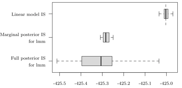
Figure1shows the variation in 50 Monte Carlo replicates of each importance sampling estimator, based on 1000 samples. The importance sampling estimates for the linear model fall close to the true log marginal likelihood value, indicated by a dashed ver-tical line. For the linear mixed model treating the random effects as missing data and drawing them from their full conditional distribution greatly reduces the variance of the importance sampling estimator. The Monte Carlo standard errors for the linear model and linear mixed model with missing data were 0.0123 and 0.0171, compared with 0.106 for the linear mixed model with an importance proposal for the full parameter vector.
Figure 1: Variation of the log marginal likelihood estimates for the linear model and linear mixed model (lmm) over 50 replicates. For the lmm, in the full posterior approach the whole parameter vector (including random effects) was approximated in the impor-tance proposal; in the marginal posterior approach the random effects were left out, and drawn from their full conditional distribution. A dashed vertical line indicates the true log marginal likelihood for the linear model.
marginal posterior approach was 0.015, showing no increase due to the increase in missing data. For comparison, the Monte Carlo standard error for the full parameter importance sampling approach increased to 0.825 form= 500.
The precision of the marginal likelihood estimator is important when it comes to estimating the Bayes factor. With m = 50 clusters the 50 Monte Carlo estimates of Bayes factor in favour of the linear model (from the missing data approach) fall between 1.279 and 1.359 for the marginal posterior importance sampling estimator. When the full posterior importance sampling estimator is used the 50 Bayes factors fall between 1.032 and 1.664, and it’s not hard to envisage situations in which this loss of precision could lead to an incorrect conclusion.
4
Final outcome epidemic data
arbitrary, but specified, non-negative probability distributionQwithE[Q] = 1 and dur-ing their infectious period make contact with a given susceptible in their household at the points of a homogeneous Poisson point process with rateλL. The special case where
Q≡1 has the same final outcomes in terms of those infected as a household Reed-Frost model within household infection probabilitypL= 1−exp(−λL). Throughout we assign an Exp(1) prior to λL which corresponds to a U(0,1) prior onpL and also a U(0,1) prior on pG.
For the household Reed-Frost epidemic it is trivial to adapt the approach of Neal and Kypraios (2015), Section 3.3 to compute the marginal likelihood exactly. Details of how this can be done are given in the supplementary material (Touloupou et al.,
2017). Therefore we are able to compare our estimation of the marginal likelihood with the exact marginal likelihood. The exact computation of the marginal likelihood grows exponentially in the total number of households whilst the MCMC algorithm for estimating the parameters and the algorithm for estimating the marginal likelihood have essentially constant computational cost for a given maximum household size. Therefore the exact computation of the marginal likelihood is only practical for data containing a small number of households and we apply it to the influenza data sets from Seattle, reported in Fox and Hall (1980), which contain approximately 90 households each.
Exact computation of the marginal likelihood is not possible for generalQ. Therefore we use our approach to compare three different choices of infectious period Q ≡ 1, Q∼Gamma(2,2) andQ∼Exp(1) to study which infectious period distribution is most applicable for a given epidemic data set. This mimics analysis carried out in Addy et al. (1991) in a maximum likelihood framework where two infectious periods, a constant and a gamma with shape parameter 2, were compared for a combined data set of two influenza outbreaks in Tecumseh, Michigan, see Monto et al. (1985).
Letxdenote the observed epidemic data. The recursive equations given in Ball et al. (1997), (3.12), can be used to computePh
k (h= 1,2, . . .;k= 0,1, . . . , h), the probability of observing k individuals out of hbeing infected in a household of size h. Therefore it is straightforward to compute π(x|λL, pG) orπ(x|pL, pG) for the Reed-Frost model. Consequently, it is trivial to construct a random walk Metropolis algorithm to sample fromπ(λL, pG|x) (orπ(pL, pG|x) for the Reed-Frost model) and to estimate the marginal likelihood using samples from a proposal density q(λL, pG), which is a multivariate t distribution with 10 degrees of freedom and mean and covariance matrix obtained from the MCMC samples.
and Ball et al. (1997). InterestinglyQ ∼Exp(1) is preferred for the Seattle influenza A and Tecumseh data sets, whereas Q ≡ 1 is Seattle influenza B data set. For the two Seattle data sets we also computed the exact log marginal likelihoods,−15.08 and −24.98, for the household Reed-Frost model applied to the Seattle influenza A and influenza B data sets, respectively. For the Seattle data sets we repeated the estimation of the log marginal likelihood 100 times for the Reed-Frost model to obtain Monte Carlo standard errors for the estimated log marginal likelihoods of 0.0062 and 0.0073 for the Seattle influenza A and Seattle influenza B data sets, respectively, demonstrating good agreement between the estimated and exact log marginal likelihoods. The calculations of the exact marginal likelihood took approximately 0.5 and 14 seconds for the Seattle influenza A and influenza B data sets, respectively. The code for computing the exact marginal likelihood could not be applied to the combined Tecumseh data set, or even the separate Tecumseh data sets (see, for example Clancy and O’Neill, 2007) since enumerating over all possible augmented data states exceeded R’s memory allocation. This problem could be circumvented to some extent using sufficient statistics as in Neal and Kypraios (2015) but the current approach offers a simple and fast alternative.
[image:12.612.183.431.322.373.2]Data Set Q∼Exp(1) Q∼Gamma(2,2) Q≡1 Seattle A -14.69 -14.86 -15.08 Seattle B -25.27 -25.11 -24.99 Tecumseh -45.58 -45.59 -45.87
Table 1: Estimated log marginal likelihood for the three influenza data sets using the three choices of infectious period distribution; Q ∼ Exp(1), Q ∼ Gamma(2,2) and Q≡1.
5
Longitudinal epidemic model
5.1
Introduction
In this Section, we explore the application of the methodology developed in Section2to a scenario whereπ(x|θ) is not readily available, and data augmentation is required both with in the MCMC algorithm and estimation of the marginal likelihood. The example used is based on a longitudinal household study of preschool children under 3 years old and all household members was conducted in the United Kingdom from October 2001 to July 2002 (Hussain et al.,2005). The size of the families varied from 2 to 7, although in most there were 3 or 4 members. All family members were examined forStreptococcus pneumoniae carriage (Pnc) using nasopharyngeal swabs once every 4 weeks over a 10-month period. The carriage status of each individual was recorded at each occasion as 1, if a carrier or 0, if a non-carrier.
as ‘adults’), denoted byi= 1,2, respectively. LetI1(t) andI2(t) denote the numbers of carrier children and carrier adults in the household at time t. The transition between state 0 and 1 is referred to as an infection and the reverse transition is referred to as clearance. The transition probabilities between states in a short time interval δt are defined for an individual in the age group i:
P(Infection in (t, t+δt]) = 1−exp
−
ki+
β1iI1(t) +β2iI2(t) (z−1)w
δt
, (16)
P(Clearance in (t, t+δt]) = 1−exp(−μi·δt), (17)
where μi and ki are the clearance and the community acquisition rates respectively for age groupi andz is the household size. The rateβij is the transmission rate from an infected individual in age group i to an uninfected individual in age group j. The term (z−1)w in (16) represents a density correction factor, where w corresponds to the level of density dependence and (z−1) is the number of other family members in a household size z. For example, w= 1 represents frequency dependent transmission, where the average number of contacts is equal for each individual in the population. Finally, the probability of infection at the initial swab is assumed to beπifor age group
i. We refer to this model asM1.
Given the dependence of the carriage status of all individuals in a household, the within household carriage dynamics in a household of sizezcan be modelled as a discrete time Markov chain with 2zstates (all possible binary vectors of infectious statuses of the
z individuals). The presence of unobserved events, that may have occurred in between swabbing intervals, has been discussed previously (Auranen et al., 2000), and must be considered in setting up the model. The approach adopted in this paper to overcome this issue is to use Bayesian data augmentation methods. Model fitting is performed within a Bayesian framework using an MCMC algorithm, imputing the unobserved carriage states in each household. LetOj⊆ {1,2, . . . , T}denote the set of prescheduled observation times of household j = 1,2, . . . , J, and let Uj ={1,2, . . . , T} \Oj denote the unobserved times. Let xj,tbe the binary vector of carriage states for individuals in householdjat observation timet. The observed longitudinal dataX= [xj,t]t∈Oj;j=1,...,J consists of the household carriage statuses xj,t at the observation times. Similarly let yj,t be the corresponding latent carriage status of householdj at timet∈Uj, and form the corresponding missing data matrix Y= [yj,t]t∈Uj;j=1,...,J. Letθ denote the vector of model parameters, including the rates of acquiring and clearing carriage, the density correctionwand the initial probabilities of carriage.
5.2
Markov chain Monte Carlo algorithm
In the Bayesian approach, the missing data is represented as a nuisance parameter and inferred from the observed data like any other parameter. The joint posterior density of the latent carriage statesy, and the model parametersθ can be factorized as:
π(y,θ|x)∝P(y,x|θ)π(θ)
=π(θ) J
j=1 T
t=1
P(zj,t|zj,t−1,θ),
where zj,t equalsxj,tift∈Oj;yj,t ift∈Uj and∅ift= 0. This factorization is based on the assumption that conditionally on the model parameters, the carriage process is assumed to be independent across households.
In order to simulate from the posterior distribution, we construct an MCMC algo-rithm that employs both Gibbs and Metropolis-Hastings updates. The main emphasis is on sampling the unobserved carriage processy, which we do using a Gibbs step via the Forward Filtering Backward Sampling (FFBS) algorithm (Carter and Kohn, 1994). In the first part of this algorithm, recursive filtering equations (Anderson and Moore,1979) are used to calculateP(yj,t|zj,t+1,xj,Oj∩{1:t},θ) for eacht ∈Uj working forwards in time. The second part then works backwards through time, simulating yj,t from these conditionals, starting with t= max(Uj) and ending witht= min(Uj). The model pa-rametersπ1andπ2are updated using Gibbs updates and the remaining parameters are updated jointly using an adaptive Metropolis-Hastings random walk proposal (Roberts and Rosenthal,2009).
5.3
Marginal likelihood estimation via importance sampling
The availability of the full conditional distribution of the missing dataP(y|x,θ) from the FFBS algorithm allows the missing data componentyto be updated using a Gibb’s step in the MCMC algorithm. This full conditional can be exploited further in the estimation of the marginal likelihood. We requireP(x|θ) in order to form the importance sampling estimator in (4). Using Bayes’ Theorem we can rewrite this as
P(x|θ) = P(x|y,θ)P(y|θ) P(y|x,θ) =
P(x,y|θ)
P(y|x,θ), (18) for any y such thatP(y|x,θ)>0. Therefore evaluation of P(x|θ) at the point θ can be done by evaluating the right-hand-side of (18) with any suitable y. A suitable y is guaranteed if it is sampled from the full conditional distributiony|(x,θ).
Sampling algorithm. We then use these samples to calculate the importance sampling estimator of the marginal likelihood:
Pq(x) = 1 N
N
i=1
P(x,yi|θi)
P(yi|x,θi)
π(θi)
q(θi)
. (19)
The choice ofq(θ) is important for the accuracy and computational efficiency of the importance sampling approach. As discussed earlier, we wantq(θ) to be a good approx-imation ofπ(θ|x) but with heavier tails to ensure that the variance of Pq is small. We therefore investigate a range of proposals distributions based on a fitted multivariate normal distribution with meanμand covariance matrixΣbased on the MCMC output. These include drawingθ fromISNj :N(μ, jΣ) (j= 1,2,3), a multivariate Normal dis-tribution with different variances;IStd:td(μ,Σ) (d= 4,6,8), a multivariate Student’s tdistribution withddegrees of freedom, meanμand covariance matrix d−d2Σ(ifd >2) andISmix :q(θ) = 0.95×N(θ;μ,Σ) + 0.05×π(θ) (mixture of a multivariate Normal density and the prior).
5.4
Marginal likelihood estimation
We consider the problem of estimating the marginal likelihood under the model in-troduced in Section 5.1, using the methods described above. These estimators were evaluated on synthetic data analogous to the real data in Melegaro et al. (2004). More specifically, the parameter values were based on the maximum likelihood estimates from the analysis of Pnc data; parameters were chosen to be k1 = 0.012, k2= 0.004, β11 = 0.047, β12= 0.005, β21 = 0.106, β22= 0.048, μ1= 0.020, μ2= 0.053, w= 1.184, π1= 0.425 and π2 = 0.095. We set the time-interval δt = 7. Only complete family transi-tions, where the infection state of all household members was known on two consecutive observations, were used previously (Melegaro et al.,2004; 51% of the full dataset). Al-though our approach could easily handle the missing data, for comparability we match the number of complete transitions by family size and number of adults to generate our data set; a total of 66 families comprising 260 individuals including 94 children under 5 years. The simulations were designed so that real and simulated datasets have the same sampling times. The hidden variable y consists of 1650 yj,t’s, comprising 6500 unobserved binary variables in total.
We compare the proposed importance sampling approach for estimating the marginal likelihood (based on the 7 proposal densities) with bridge sampling (Meng and Wong,
1996) (using the importance samples fromISmix), harmonic mean (Newton and Raftery,
1994), Chib’s method (Chib,1995; Chib and Jeliazkov,2001) and the power posteriors method (Friel and Pettitt, 2008). Details of the computation of these estimators are given in the supplementary material (Touloupou et al.,2017). To compare the different methods on a fair basis, we chose to dedicate equivalent amounts of computational effort for estimation of the log marginal likelihood, instead of fixing the total number of samples.
MCMC sampler described in Section5.2. These posterior samples were used to estimate the reference parameters μ and Σ for a multivariate Student’s t or normal proposal density. The marginal likelihood estimate was then based on 25000 importance sampling draws from the obtained proposal densityq(θ), using the estimator in (19). To produce the bridge sampling estimate, the 25000 samples from ISmix were combined with 250 thinned samples from the MCMC. In order to apply Chib’s methods, the same posterior samples were used for computing the high posterior density point. The log marginal was estimated by generating 22000 draws in each complete and reduced MCMC run, with the first 2000 draws removed as burn-in. Harmonic mean analysis was based on 50000 posterior samples, following a 3000 iteration burn-in. For the power posterior method, it was necessary to specify the temperature scheme and a pilot analysis (not counted in the computation cost) was used to choose 20 partitions on the unit interval. The MCMC sampler was run for 2650 iterations for each temperature in the descending series, omitting the first 650 as burn-in, finishing with 2650 samples at t = 0 (the prior).
Each procedure was repeated 50 times to provide an empirical Monte Carlo estimate of the variation in each approach. We also vary the total running time in order to investigate the effect of this on the accuracy of the marginal likelihood estimates, see Table 1 in the supplementary material. For each analysis method we used the same priors: Gamma(0.01,0.01) for the density factorw; Beta(1,1) for the initial probabilities of infectionπ1and π2 and Gamma(1,1) for the remaining parameters.
Figure2 shows the variability of the eleven marginal likelihood estimators. Except for the harmonic mean, all the methods appear to have produced consistent estimates of the marginal likelihood. Chib’s method produced better estimates of the marginal likelihood than the power posterior method, which is more computationally expen-sive than the other methods and therefore uses a small number of MCMC samples at each temperature, leading to large uncertainty. However as seen in Figure2, the bridge sampling and the importance sampling methods offer significant improvements in pre-cision over the other methods. Moreover, increasing the number of samplesN, led to a decrease in the Monte Carlo standard errors of order O(√N), see Table 1 in the sup-plementary material, indicating that the variances of the corresponding estimators are finite.
The success of the importance sampling approach is not surprising since it explores the posterior distribution of parameters more efficiently than the other methods due to the independence of the samples drawn from the proposal density. More surprisingly we were unable to use the bridge sampling technique to improve substantially on the standard errors, which dropped from 0.0196 forISmix to 0.0179 forBSmix. The bridge sampling estimator attempts to combine information from the MCMC and importance samples, however the optimal estimator is derived assuming that independent samples from the posterior were available, which we approached by applying a thinning of 100 to the samples. With low levels of thinning (results shown in supplementary material Figure 4) we found that bridge sampling actually increased the standard error of the marginal likelihood estimate.
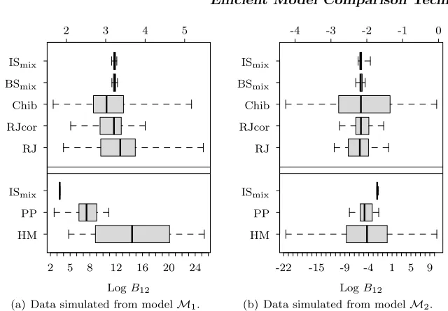
Figure 2: Top: Boxplots of the estimated log marginal likelihood for modelM1 over 50 replicates for our importance sampling approach with the mixture proposal (ISmix), Chib’s method (Chib), power posteriors method (PP) and harmonic mean (HM) (note the different scales for the top and bottom plots). Bottom: Zoomed in boxplots of the estimated log marginal likelihood for model M1 over 50 replicates for each of our importance sampling approach (ISN1, ISN2, ISN3, ISt4, ISt6, ISt8, ISmix) and bridge sampling (BSmix).
5.5
Model comparison
In this Section, we apply the marginal likelihood estimation approaches to the problem of Bayesian model choice. We focus on their ability to distinguish between biologically motivated hypotheses concerning the dynamics of Pnc transmission. In particular we compare their performance against the established technique of Reversible Jump Markov Chain Monte Carlo (RJMCMC) and then demonstrate that the importance sampling approach can solve problems that are extremely challenging with RJMCMC. We show that using our approach it is possible to answer the epidemiological important question of how household size is related to transmission with extended discussion given in the supplementary material.
Suppose that we wish to evaluate the evidence in favour of the community acquisition rates being equal for adults and children, in the hope of developing a more parsimonious model. We call the model described in Section 5.1, in which children have community acquisition ratek1and adults have ratek2, modelM1. The nested model, in whichk1= k2 is called M2. We generated realistic simulated datasets from each of these models and then used importance sampling, bridge sampling, Chib’s method, power posteriors, the harmonic mean and reversible jump MCMC to estimate the Bayes factor in favour of M1, denoted byB12. As before, we used approximately the same computational effort for each of these approaches. ForM1we assumedk1= 0.012 andk2= 0.004, whilst for M2 we assumedk1=k2= 0.008.
Details of the RJMCMC algorithm for selecting between models M1 and M2 are given in the supplementary material. We ran the RJMCMC chain with a 30000 burn-in followed by 76000 samples which ensured that similar computational effort was given to RJMCMC as to the other methods. When the evidence is strongly in favour of one model, the RJMCMC will not move between models very often and can provide poor estimates of the Bayes factor. A variant of the method, called RJMCMC corrected (RJcor), can tackle this issue by assigning higher prior probability to the model that is visited less often. This probability is estimated asπ(Mm) = 1−π(Mm|x), where
π(Mm | x) is obtained from a pilot run of RJMCMC with initial π(Mm) = 0.5, for
m= 1,2. For RJcor we did 30000 pilot iterations and then another 76000 iterations, of which 30000 were discarded as a burn in.
Figure 3: Variability of the log Bayes factor estimates based on 50 Monte Carlo repeats for the importance sampling method with mixture proposals (ISmix), bridge sampling method with mixture proposals (BSmix), Chib’s method (Chib), reversible jump MCMC (RJ), corrected reversible jump MCMC (RJcor), power posteriors (PP) and harmonic mean (HM) methods (note the different scales for the top and bottom plots).
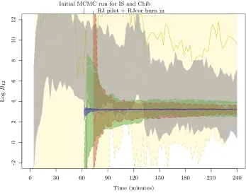
Figure 4 demonstrates the evolution of the log Bayes factor in favour of M1 as a function of computation time using data generated fromM1. The importance sampling estimator (in blue) converges much more rapidly than the other estimators, showing very tight credible intervals. Chib’s method (in green) and corrected RJMCMC (in red) appear to converge to the same value, but more slowly and have wider CIs. The power posterior method gradually approaches the consensus estimate, requiring significantly more samples to stabilize. The harmonic mean estimator was heavily unstable and also provided much wider credible intervals than the other methods.
In the supplementary material (Touloupou et al.,2017), further model comparison questions are considered and the strength of the importance sampling technique for an-swering these questions is further demonstrated. In particular, we consider heterogeneity in household transmission rates, density-dependence in within-household transmission and the amount of missing data.
6
Conclusions
Figure 4: Evolution of log Bayes factor estimates in favour of model M1 as a func-tion of computafunc-tion time. The solid lines corresponds to the median and the shaded areas give the 95% credible intervals, estimated from 50 Monte Carlo replicates. Yellow represents the harmonic mean method, grey is for the power posterior, red and green correspond to RJMCMC corrected and Chib’s methods respectively and blue represents the importance sampling approach with the mixture proposals.
sample from and an effective estimate of the likelihood π(x|θ). The first observation is whilst an MCMC algorithm will often be relatively straightforward to construct, alter-native methods for sampling from the posterior distribution could be equally considered. Moreover, it is not important if a sample from an approximate posterior distribution (for example, Monte Carlo within Metropolis; O’Neill et al., 2000) is used since all that is required for computation of the marginal likelihood is to be able to make a reasonable choice ofq(·). The key limitation to using this approach is effective estima-tion of the likelihood π(x|θ) in cases where it is not analytically tractable. In Section
Supplementary Material
Supplementary material: Efficient model comparison techniques for models requiring large scale data augmentation (DOI:10.1214/17-BA1057SUPP; .pdf).
References
Addy, C. L., Longini, I. M. and Haber, M. (1991). A generalized stochastic model for the analysis of infectious disease final size data.Biometrics 47, 961–974. 9,10
Anderson, B. D. O. and Moore, J. B. (1979). Optimal filtering.Englewood Cliffs, New Jersey: Prentice Hall. 13
Auranen K., Arjas E., Leino T. and Takala A. K. (2000). Transmission of pneummono-coccal carriage in families: A latent Markov process model for binary longitudinal data. Journal of the American Statistical Association 95, 1044–1053. MR1821713. doi:http://dx.doi.org/10.2307/2669741. 12
Ball, F. G., Mollison, D. and Scalia-Tomba, G. (1997). Epidemics with two levels of mixing. The Annals of Applied Probability 7, 46–89. MR1428749. doi:http://dx.doi.org/10.1214/aoap/1034625252. 10,11
Carter, C. K. and Kohn, R. (1994). On Gibbs sampling for state space models. Biometrika 81, 541–553. MR1311096. doi: http://dx.doi.org/10.1093/biomet/ 81.3.541. 5,12,13
Chen, M.-H. (2005). Computing marginal likelihoods from a single MCMC output. Statistica Neerlandica 59, 16–29. MR2137379. doi: http://dx.doi.org/10.1111/ j.1467-9574.2005.00276.x. 2
Chib, S. (1995). Marginal likelihood from the Gibbs output. Journal of the American Statistical Association 90, 1313–1321.MR1379473. 2,14
Chib, S. and Jeliazkov, I. (2001). Marginal likelihood from the Metropolis-Hastings output. Journal of the American Statistical Association 96, 270–281. MR1952737. doi:http://dx.doi.org/10.1198/016214501750332848. 2,14
Clancy, D. and O’Neill, P. (2007). Exact Bayesian inference and model selection for stochastic models of epidemics among a community of households. Scandinavian Journal of Statistics 34, 259–274. MR2346639. doi:http://dx.doi.org/10.1111/ j.1467-9469.2006.00522.x. 11
Clyde, M. A., Berger, J. O., Bullard, F., Ford, E. B., Jefferys, W. H., Luo, R., Paulo, R. and Loredo, T. (2007). Current challenges in Bayesian model choice. InStatistical Challenges in Modern Astronomy IV ASP Conference Series, Vol. 371, proceedings of the conference held 12–15 June 2006 at Pennsylvania State University, in University Park, Pennsylvania, USA. Edited by G. Jogesh Babu and Eric D. Feigelson.p. 224.
Doucet, A. and Johansen, A. M. (2011). A tutorial on particle filtering and smoothing: fifteen years later. In Handbook of Nonlinear Filtering (eds D. Crisan and B. Rozovsky). Cambridge: Cambridge University Press. pp. 656–704.
MR2884612. 4
Fong, Y., Rue, H. and Wakefield, J. (2010). Bayesian inference for generalized linear mixed models.Biostatistics 11, 397–412. 6
Fox, J. P. and Hall, C. E. (1980). Viruses in families.PSG Publishing, Littleton, MA.
10
Friel, N. and Pettitt, A. N. (2008). Marginal likelihood estimation via power posteriors. Journal of the Royal Statistical Society: Series B (Statistical Methodology) 70, 589– 607. MR2420416. doi: http://dx.doi.org/10.1111/j.1467-9868.2007.00650.x.
2,14
Gelfand, A. E. and Dey, D. K. (1994). Bayesian model choice. Exact and asymptotic calculations. Journal of the Royal Statistical Society. Series B (Methodological)56, 501–514. MR1278223. 2,3
Gordon, N. J., Salmond, D. J., and Smith, A. F. M. (1993). Novel approach to nonlinear/non-Gaussian Bayesian state estimation.Radar and Signal Processing, IEE Proceedings F 140, 107–113. 5
Green P.J. (1995). Reversible jump Markov chain Monte Carlo computation and Bayesian model determination. Biometrika 82, 711–732. MR1380810. doi:http://dx.doi.org/10.1093/biomet/82.4.711. 2, 6
Hastings, W. (1970). Monte Carlo sampling methods using Markov chains and their ap-plications.Biometrika 57, 97–109. MR3363437. doi:http://dx.doi.org/10.1093/ biomet/57.1.97. 2
Hesterberg, T. (1995). Weighted average importance sampling and defense mixture dis-tributions.Technometrics 37, 185–194. 3
Hussain M., Melegaro A., Pebody R. G., George R., Edmunds W. J., Talukdar R., Martin S. A., Efstratiou A. and Miller E. (2005). A longitudinal household study ofStreptococcus pneumoniae nasopharyngeal carriage in a UK setting.Epidemiology and Infection 5, 891–898. 11
Karagiannis, G., and Andrieu, C. (2013). Annealed importance sampling reversible jump MCMC algorithms. Journal of Computational and Graphical Statistics 22, 623–648.
MR3173734. doi:http://dx.doi.org/10.1080/10618600.2013.805651. 2
Kass, R. E. and Raftery, A. E. (1995). Bayes factors. Journal of the American Sta-tistical Association 90, 773–795. MR3363402. doi: http://dx.doi.org/10.1080/ 01621459.1995.10476572. 2
Melegaro, A., Gay, N., and Medley, G. (2004). Estimating the transmission parameters of pneumococcal carriage in households. Epidemiology and Infection 132, 433–441.
3,11,14
Metropolis N., Rosenbluth A., Rosenbluth M., Teller A. and Teller E. (1953). Equations of state calculations by fast computing machines. Journal of Chemical Physics 21, 1087–1092. 2
Meng, X.-L. and Wong, W. H. (1996). Simulating ratios of normalizing constants via a simple identity: A theoretical exploration. Statistica Sinica 6, 831–860.MR1422406.
2,12,14
Monto, A. S., Koopman, J. S. and Longini, I. M. (1985). Tecumseh study of illness. XIII. Influenza infection and disease, 1976–1981.American Journal of Epidemiology
121, 811–822. 10
Neal, P. and Kypraios, T. (2015). Exact Bayesian inference via data augmenta-tion.Statistics and Computing 25, 333–347 MR3306710. doi:http://dx.doi.org/ 10.1007/s11222-013-9435-z. 9,10,11
Neal, P. and Subba Rao, T. (2007). MCMC for integer-valued ARMA processes.Journal of Time Series Analysis28, 92–110. MR2332852. doi:http://dx.doi.org/10.1111/ j.1467-9892.2006.00500.x. 6
Newton, M. A. and Raftery, A. E. (1994). Approximate Bayesian inference with the weighted likelihood bootstrap. Journal of the Royal Statistical Society. Series B (Methodological)56, 3–48.MR1257793. 14
O’Neill, P. D., Balding, D. J., Becker, N. G., Eerola, M. and Mollison, D. (2000). Analy-ses of infectious disease data from household outbreaks by Markov Chain Monte Carlo methods. Journal of the Royal Statistical Society. Series C (Applied Statistics)49, 517–542. MR1824557. doi:http://dx.doi.org/10.1111/1467-9876.00210. 19
Ripley, B. D. (1987). Stochastic Simulation. Wiley & Sons. MR0875224. doi:http://dx.doi.org/10.1002/9780470316726. 3
Roberts, G. O. and Rosenthal, J. S. (2009). Examples of adaptive MCMC. Journal of Computational and Graphical Statistics 18, 349–367 MR2749836. doi:http://dx.doi.org/10.1198/jcgs.2009.06134. 13
Skilling, J. (2004). Nested sampling. AIP Conference Proceedings 735, 395–405.
MR2266273. doi:http://dx.doi.org/10.1063/1.1835238. 2
Smith, M. and Kohn, R. (1996). Nonparametric regression using Bayesian variable se-lection.Journal of Econometrics 75, 317–344. 7
Tierney, L. and Kadane, J. B. (1986). Accurate approximations for posterior moments and marginal densities. Journal of the American Statistical Association 81, 82–86. 590–599. MR0830567. 3
requir-ing large scale data augmentation. Bayesian Analysis. doi: http://dx.doi.org/ 10.1214/17-BA1057SUPP. 8,10,14,18
Zeger, S. (1988). A regression model for time series of counts.Biometrika 75, 621–629.
MR0995107. doi:http://dx.doi.org/10.1093/biomet/75.4.621. 5,6
Zhou, Y., Johansen, A. M. and Aston, J. A. D. (2015). Towards automatic model comparison: An adaptive sequential Monte Carlo approach. Journal of Computa-tional and Graphical Statistics 25, 701–726. MR3533634. doi:http://dx.doi.org/ 10.1080/10618600.2015.1060885. 2
Acknowledgments
PT was supported by a University of Warwick PhD scholarship. NA was supported by a PhD scholarship from the Saudi Arabian Government. PN, SS and TM would like to thank the organisers of the Design and Analysis of Infectious Disease Studies workshop at Oberwolfach (November 2013), where many helpful discussions took place.