https://doi.org/10.1007/s00355-019-01178-6
O R I G I N A L P A P E R
How should payment services be taxed?
Ben Lockwood1 ·Erez Yerushalmi2
Received: 14 April 2018 / Accepted: 31 January 2019 © The Author(s) 2019
Abstract
This paper considers the design of taxes on real money balances and bank payment ser-vices, when realistically, the household can use either cash or a bank payment account for the purchase of different varieties of goods. These taxes, plus a consumption tax, fund a government revenue requirement. We find that generally, real money balances and bank transaction fees should be taxed, and at different rates, i.e. the tax system should not leave the choice of payment services undistorted. For a wide class of time transactions cost technologies, including the Baumol-Tobin case, fees should be taxed at a lower rate than real money balances, and the tax on real money balances should be positive. However, it is possible that fees should be subsidized. The rate of tax on fees has no simple relationship to the optimal consumption tax, and can be higher or lower. A Corlett-Hague type intuition for these results is also developed, which relies on the concept of a virtual time endowment.
JEL Classification G21·H21·H25
This paper is a substantially revised version of Centre for Business Taxation Working Paper 1423, ”Should transactions services be taxed at the same rate as consumption?”, published in 2014. We would like to thank Robin Boadway, Steve Bond, Clemens Fuest, Michael Devereux, Andreas Haufler, Michael McMahon, Miltos Makris, Ruud de Mooij, Carlo Perroni, and seminar participants at the University of Southampton, GREQAM, the 2010 CBT Summer Symposium, the 2011 IIPF Conference and OFS workshop on Indirect Taxes for helpful comments on earlier drafts. Ben Lockwood also gratefully acknowledges support from the ESRC grant RES-060-25-0033, ”Business, Tax and Welfare”.
Electronic supplementary material The online version of this article ( https://doi.org/10.1007/s00355-019-01178-6) contains supplementary material, which is available to authorized users.
B
Ben LockwoodErez Yerushalmi
1 CBT, CEPR and Department of Economics, University of Warwick,
Coventry, England CV4 7AL, UK
1 Introduction
This paper addresses a relatively neglected issue, the optimal taxation of payment services. By payment services, we mean the services provided by the banking system that facilitate payment for goods and services. There is of course, a large literature on the optimal taxation of fiat money, the so-called inflation tax literature. This literature focuses on conditions for the zero taxation of cash, i.e. the Friedman rule, which says that the nominal interest rate should be zero. In this literature, however, it is assumed, without exception, that cash is the only medium of payment, or that some goods can be bought on credit, and so the issue of how services provided by the banking system should be taxed is not addressed.1
This focus on cash may have been justified years ago, when the use of a bank account meant the writing of a check, and most transactions were made using cash. However, the focus on the literature on cash is clearly increasingly unrealistic because technological advances have allowed so-called electronic transfer of funds at the point of sale, by using credit and debit cards. These services are rapidly overtaking cash as means of payment for retail transactions.2
For example, based on a large-scale payment diary survey, conducted between 2009 and 2012 in seven major countries, Bagnall et al. (2016) report that the share of the number of transactions with cash is on average of 62% (between 46 and 82%, varying by country), while its value share is on average of 35% (between 15 and 65%).3As expected, this shows that a larger number of smaller transactions are made by cash, and that larger value transactions are made by other means. In recent years, the share of cash has fallen further. For example, in the US, the share of cash in retail transactions fell from 40% in 2012 to 32% in 2015 (Matheny et al.2016).
On the other hand, it is unlikely that cash will disappear altogether as a medium of payment; as reported by the Cash Product Office of the US Federal Reserve, “In 2015, cash continued to dominate small-value transactions, with cash being used for more than 50% of transactions under $25....(and) for more than 60% of purchases under $10.” (Matheny et al.2016, p6). Again, in another large scale payment diary survey in the Euro Area in 2016, for a subset of EU countries, Esselink and Hernández (2017) report an even higher ratio of cash usage than Bagnall et al. (2016), for countries such as Cyprus, Greece, and Malta, which used above 70% cash by transactions value.
1 See for example, Correia and Teles (1996, 1999) which consider a transactions cost theory of money
demand, or Chari et al. (1991, 1996), where some goods can be bought on costless credit. More recent models include a more micro-founded search theoretic demand for fiat money e.g. Aruoba and Chugh (2010), but existing models of this type do not include a banking sector. The literature is surveyed in Kocherlakota (2005) and Schmitt-Grohe and Uribe (2010).
2 As a result of these trends, the provision of payment services is an increasing source of both activity
and profit for banks and payment network operators, such as VISA and Mastercard. For example, in the United States, the fee averages approximately 2% of transaction value. This is giving rise to large and growing revenues and profits for both banks and the operators. For example, DeYoung and Rice (2004) estimate that in the US in 2003, non-interest income accounted for half of all bank income, and 52% of non-interest income was generated by fees associated with payment accounts. Visa, the largest payment network operator, had gross income and profit of $18.36 bln. and $11.69 bln. in the 2017 financial year.
Does the choice of payment method matter? At a macroeconomic level, Philippon (2015) and Bazot (2018), show that the costs of financial intermediation for the banking sector in the US and Europe are considerable; for the US, they estimate these costs at around 2.5% of assets intermediated. The specific costs of operating payments services such as Mastercard, Visa etc are also large; for example a 2012 study by the European Central Bank estimated the average resource cost of non-cash payment systems across EU-27 at about 1% of GDP (Schmiedel et al.2012). This translates to about 2.8% of the value of consumption facilitated by payments systems.4But, these costs have to be set against the benefits to consumers in terms of greater time saving, convenience, and security.
Given these two methods of payment for goods, the question then arises as to how they should be taxed, if a government has to use distortionary taxes to raise revenue. This paper studies the optimal tax structure in a model that combines the transaction cost theory of the demand for money (for example Correia and Teles (1996), Teles (2003)), with the model of Freeman and Kydland (2000), which allows for substitution between cash and use of bank accounts. In our model, the household demands different varieties of goods in different quantities, and these can be paid for either by cash, or by electronic transfer of funds at the point of sale, provided by a bank account. We will call this account apayment account(PA).5
The time transactions cost of using cash is modeled in the usual way, by assuming that goods bought with cash require a time input from the household, which can be lowered by holding a higher stock of real money balances.
We model the cost of using a PA by assuming that the bank charges a per transaction fee to the seller of the good, which is then passed on to the consumer by the seller.6 To make our point as clearly as possible, we assume the use of the PA requiresno time inputfrom the household. While this is an abstraction, it is increasingly close to reality, with so-called ”contactless” payment via debit card, and mobile phone apps for management of bank accounts becoming increasingly widespread.
To ensure that the choice between cash and a PA is not trivial, we assume that cash has a real resource cost, as in Correia and Teles (1996). The reason for this is that if cash were free, the optimal inflation tax would be zero, and then the household would use only cash.7We then show that in equilibrium, there will be a ”switch point” above which varieties in greater demand will be bought using the PA.
The government has a fixed revenue requirement in each period, and to finance this, can tax the payment fees charged by banks, and can also tax real money balances via an inflation tax. In addition, the government has the use of a consumption or income tax. In this setting, we characterize optimal payment service taxes i.e. the structure of taxes on both real money balances and the fees, as well as the consumption tax.
4 On average, in the EU, consumption is about 70% of GDP. Also, as a rough approximation, about 50%
of total transactions are non-cash. So, the percentage is 1%/(0.7×0.5)=2.8%.
5 So, a payment account is what is known as a checking account in the USA, and a current account in the
UK.
6 These fees are known as merchant discount fees. The bulk of this is made up of a change for card use by
the card-issuing bank, known as the interchange fee, and the reminder of the merchant discount fee goes to the card company and the acquiring bank.
Our main contribution is to develop simple formulae for the optimal ad valorem taxes on both real money balances and transactions fees. It turns out that the structure of taxes on these two payment methodsonlydepend on the characteristics of the time transactions cost of cash,notthe form of the household utility function.
Specifically, in our setting, the time used for transactions is a function of the quantity of goods bought with cash (cash purchases), and real money balances. Then, both the sign of each tax, and the ratio of these two taxes, depend only on the properties of the time transactions cost function. Assuming that this function is homogeneous of degree k,both taxes are decreasing ink.The tax on cash is also increasing in elasticity of the marginal time transactions cost of additional cash purchases with respect to real money balances. Similarly, the tax on fees is also increasing in elasticity of the marginal time transactions cost of additional cash purchases with respect to cash purchases. Ifk≤1, the tax on real money balances is always positive, but the tax on fees may be negative. We also find conditions on the time transactions cost of cash such that the taxes are positive, and that the tax on cash is always higher than the tax on fees.
The general intuition for these results is based on the concept of a “virtual” time endowment. Specifically, we can reduce the tax design problem for the government to a completely standard one, except that the household has, instead of a fixed time endowment, a “virtual” time endowment that is endogenous, and depends onkand the share of goods bought with cash and real money balances. This virtual time endowment is of course not directly taxable, but can be indirectly taxed by taxes on payment services insofar as they affect the share of goods bought with cash and real money balances. For example, a tax will be positive if it indirectly reduces the virtual time endowment. Thus, in general terms, the intuition is similar to that of Corlett and Hague (1953), who argue that taxes should be set to indirectly tax non-taxable leisure. However, the specific mechanism is quite different; in Corlett and Hague (1953), the key variable is the degree of complementarity in preferences between leisure and the taxed goods. Here, it is the properties of the transactions technology that are key.
We also relate our results to the Diamond and Mirrlees (1971) production efficiency result. One can interpret the transactions technology in our model as a form of house-hold production, where inputs in the form of cash balances and PAs, combined with market purchases and time, produce final consumption. Our result is thatevenwith a constant returns transactions time technology, these inputs to final consumption should generally be taxed. In other words, the Diamond–Mirrlees principle that inputs should not be taxed with constant returns in production does not extend to the household in this context.
Our results also have implications for the literature on the optimal inflation tax. For example, we show that the findings of Correia and Teles (1996) are not robust to introducing substitutability between cash and PAs.8Specifically, we show that when both payment media are used, real money balances should be taxed even whenk=1, in contrast to their findings when cash is the only medium of payment.9
8 The Correia-Teles model is a special case of ours, as explained in Sect.3.5
9 The work of Correia and Teles (1996) has already shown, however, that in an environment where only cash
We then turn to some numerical simulations, using a calibrated version of the model. We find that, consistently with our analytical results, both the inflation tax and the tax on fees decrease markedly as the returns to scale in transactions costs increase from zero to one. The results show also that both inflation tax and the tax on fees decrease as the bank fee increases. This is interesting as the move away from cash that we currently observe is ultimately driven by technological innovation that reduces fees. Moreover, when the fee is large or when returns to scale are close to one, the tax on fees can be negative i.e. bank fees should be subsidized. We also find that the tax on bank fees can be greater or less than the rate of consumption tax although both taxes are of the same order of magnitude.
Our findings have some implications for the current policy debate on the taxation of banks, especially in Europe, where it is the view of many, including the European Commission, that banks are under-taxed, because many of their services are exempt from VAT.10In this debate, it is largely assumed that within a consumption tax system, such as a VAT, it is desirable to tax financial services at the standard rate of VAT e.g. Ebrill et al. (2001).11 Our results provide some support for this position, in that we find that payment services provided by banks should be taxed positively in a number of cases.
The remainder of the paper is organized as follows. Section2provides a summary of related literature. Sections3–5outline the model. Section6presents the main results. Section7presents a calibrated version of the model, and Sect.8concludes.
2 Related literature
Our paper relates to a number of literatures. First, there is a small literature directly addressing the taxation of payment services (Grubert and Mackie2000; Jack2000; Auerbach and Gordon 2002). With the exception of Auerbach and Gordon (2002), these papers use a simple two-period consumption-savings model without an explicit production sector, and assume that payment services are consumed in fixed proportion to aggregate consumption.12In this setting, it is straightforward to show that if there is a pre-existing consumption tax at the same rate in both periods, the marginal rate of substitution between present and future consumption is left unchanged if payment services are taxed at the same rate as consumption.
Footnote 9 continued
transactions technology is decreasing returns, this creates a ”virtual profit” for the household which can be taxed via a positive inflation tax. This is, of course, analogous to the original Diamond–Mirrlees result, which states that inputs to production should be untaxed as long as there are constant returns to scale (or 100% profit taxation), but taxed if there are decreasing returns to scale (Stiglitz and Dasgupta1971).
10 Currently, within European Union countries, most financial intermediation services are exempt from
VAT, notably financial services which are not explicitly priced (De La Feria and Lockwood2010; PWC
2011; Buettner and Erbe2014).
11 See also the recent IMF proposals for a Financial Activities Tax levied on bank profits and remuneration,
one version of which - FAT1 - would work very much like a VAT (IMF2010).
12 Chia and Whalley (1999), using a computational approach, reach the rather different conclusion that no
Auerbach and Gordon (2002) consider a multi-period life-cycle model of the con-sumer where purchase of goods requires payment services, which themselves are produced using other inputs. Payment services are assumed to be demanded in strict proportion to consumption. They show that if there is initially only a labor income tax imposed on the household, then this is equivalent to a value-added tax if and only if the payment services consumed by the household are taxed at the same rate as other goods.13
There are, however, a number of restrictive assumptions implicit in these existing models. First, and foremost, they do not allow the household to choose between cash and other payment services. Second, other taxes are assumed fixed, not optimized, and it is implicit that the existing taxes are non-distortionary, because the analysis proceeds by finding conditions under which taxation of payment services does not introduce any further distortions. By contrast, we take an explicit tax design approach to the question, investigating the second-best tax structure.
The second related literature is on the optimal inflation tax. This literature is mature, and there are a number of well-known reasons why the Friedman rule may not hold and it may be optimal to tax real money balances. These include the existence of pure profit due to decreasing returns to scale, imperfect competition in the product market, or tax evasion (see for example, the surveys by Kocherlakota2005; Schmitt-Grohe and Uribe2010). Our model has none of these features, but we still find violation of the Friedman rule, for completely different reasons. Moreover, in spite of the large literature on the Friedman rule, we are not aware of any paper that studies the optimal tax structure on both cash and non-cash payment instruments.
A third related literature is the one on optimal taxation with household production (Sandmo1990; Piggott and Whalley2001; Kleven et al.2000). This literature has a number of similarities to ours. Specifically, the complementarity of purchased inputs and household time in household production is an important determinant of the optimal tax structure, and also, there is generally production inefficiency; that is, taxes distort the choice of inputs to household production. The relationship of our results to theirs is further discussed in Sect.6below.
Finally, there is a recent literature studying banks that engage in socially undesirable activities such as excessive risk-taking.14 The main finding is that these should be corrected by Pigouvian taxes (or regulations) that apply directly to these decision margins, such as taxes on borrowing or lending. Our work is distinct from this line of inquiry, as the banking sector has no external effects in our setting; we are concerned with the design of taxes to raise revenue. So, we are studying ”boring banks” in the terminology of Aigner and Bierbrauer (2015), to which our paper is also related. They, however, focus on tax incidence issues, whereas we are concerned with tax design.
13 In particular, they show that if there is initially a wage income tax at rateτ,which is replaced by a
consumption tax at equivalent rateτ/(1−τ),then the real equilibrium is left unchanged if and only if payment services are also taxed at this equivalent rate.
14 See e.g. Acharya et al. (2017), Bianchi and Mendoza (2010), Jeanne and Korinek (2010), Keen (2011),
3 The model
The model is a modified version of the Freeman and Kydland (2000) model. This model has a number of attractive features which generates an equilibrium where cash and PAs co-exist, and where small items will be purchased with cash and larger items will be purchased with PAs. These are: (i) the consumption bundle is sorted by the sizes of the purchases, (ii) there is a time cost of using cash, and (iii) there is a fixed cost per transaction of using the PA. All these features are needed for a non-trivial analysis of the effects of payment services taxes on household behavior. The exact relationship of our set-up to Freeman and Kydland (2000) is discussed further in Sect.3.5below.
3.1 Set-up
A large number of identical households live for periodst=1, . . .∞.In each period, they consume a number of different varieties of a consumption goodj ∈[0,1], supply labor, and can also hold cash, bank deposits and government bonds. The banks take deposits and use them to buy government bonds, and also provide payment services to depositors. The government issues bonds and sets taxes to finance an exogenous level of public good provision in each period.
3.2 Firms and banks
In each period, a single competitive firm produces an intermediate good from labor, where one unit of labor produces one unit of the good. One unit of this intermediate good can be transformed by a seller j into one unit of variety j ∈ [0,1] of the consumption good. All sellers are perfectly competitive price takers and thus set a price of variety j equal to the price of the intermediate good.
A single competitive bank offers a PA to the households. It takes nominal deposits Dt from the household in periodt, and purchases government bondsBtB. The bank
also provides payment services, using the intermediate good as an input. Specifically, any variety jcan be purchased using the PA at a cost of f per purchase in units of the intermediate good. As the bank is competitive, we assume that the cost is just passed on to the household, without any mark-up.
This fee can be taxed at rateτtfso the household faces a costf
1+τtf
if it chooses to purchase variety jusing a PA. We interpret f as covering all costs associated with the banking system. So, f measures, inter alia, the costs of physical bank branches, and all labor and other costs associated with PAs. Included in this would be the bank interchange fee that a card-issuing bank charges the seller of the good for the use of the card.15
15 In practice, the bank interchange fee is a fixed chargef,plus a percentage of the value of the transaction.
Finally, the stock of bonds outstanding att pay a nominal interest rateit. As the
bank is perfectly competitive, this is also the return on deposits.
3.3 Households
The single infinitely lived household has preferences over levels of consumption goods and leisuret =0, ..∞of the form:
∞
t=0 βtu(c
t,lt) , ct = min
j∈[0,1]{ct(j) /2j}, (1)
wherect(j)is the level of consumption of varietyjin periodt,ltis the consumption of
leisure. We assumeu(c,l)is strictly increasing and strictly concave, and thatucl ≥0,
where subscripts denote derivatives. Also, 0< β <1 is a discount factor.
The fixed coefficients specification for the commodity index follows Freeman and Kydland (2000); it allows for consumption levels of the different varieties to vary in an analytically tractable way. In particular, all varieties will be consumed in fixed proportions to somec, i.e.
c(j)=2cj, j∈[0,1]. (2)
Note that aggregate consumption is01c(j)d j=c.
The household can use either cash or the PA to make purchases. The advantage of using the PA is that relative to cash, it economizes on household time. To make this point as cleanly as possible, we assume that use of the PA requiresnotime. This is an increasingly close approximation to reality, as many card transactions are contactless (i.e. do not even require a security (PIN) number) and accounts can be managed via smart-phone apps. On the other hand, using cash is costly in terms of time, for several reasons that are well-documented in the literature; it has to be physically withdrawn from ATMs, stored securely, etc.
We capture this by supposing that a volumex ≡2cT j d jof consumption bought with cash requiress(x,m)units of time, whereT ⊂[0,1] is the subset of goods that are bought with cash, andmis real money balances, defined below. We assume that sis twice continuously differentiable, increasing in xand decreasing inm. We will also assume that an increase in the use of money reduces the marginal transactions cost i.e.sxm < 0. This general specification s(x,m)of the time transactions cost
of cash is standard in the literature, and includes a number of well-known special cases. For example, with the inventory-theoretic demand for money of Baumol and Tobin,shas the interpretation of the time cost of the number of trips to the bank, so s = αmx,where αis the time cost per trip, and mx is the number of trips. A rather different specification is used in the more recent literature on the optimal inflation tax; for example, Schmitt-Grohe and Uribe (2010) assumes =σmxx, whereσ(.) is strictly increasing.
subscripts denote partial derivatives, so that for examplesx = ∂∂sx. At the household
optimum, because the wage is unity, both are measured in the same units, so the net cost is f 1+τf−sx2cj. It is immediate that the net cost of using the PA is decreasing
in j,so in any periodt,there will be a critical index jt∗such that all goods j < jt∗ are bought with cash, and all goods j> jt∗are bought with the PA. This is consistent with what is observed in practice, where cash is used for small transactions, and PAs for larger transactions.16
So,xt,the volume of goods bought with cash, is
xt =2
jt∗
0
ctj d j =
jt∗
2
ct. (3)
Finally, following Correia and Teles (1996) and Teles (2003), to getmt,we deflate
nominal money holdings by the periodtprice level Pt,inclusive of the consumption
taxτtci.e.
mt =
Mt
Pt
1+τtc
.
This captures the idea that nominal money balances are needed to pay for goods where the price includes the taxτtc.
In each period, the household consumes goods and leisure, and can accumulate bonds, cash, or deposits in the PA. So, the per period budget constraint is
Ptct
1+τtc+Pt
1−jt∗ f
1+τtf
+Mt+1+Dt+1+BtH+1
=Ptht+Mt+(1+it)
BtH+Dt
, t=1,2, ... (4)
Note that1−jt∗ f
1+τtf
is the overall cost in consumption units of using a PA for varieties j ≥ jt∗.Here, labor supplyht to the intermediate good sector is the time
endowment minus leisure and the time transactions cost i.e.,
ht =1−lt−st. (5)
Also, here, Dt, BtH are holdings of deposits and bonds at timet.Finally, following
Chari et al. (1996), we assume thatM0 =D0 =B0H =0;if these initial conditions do not hold, then the government’s problem is trivial.17
16 For example, using a sample of Dutch retailers, ten Raa and Shestalova (2004) estimate that the point at
which households switch from cash to electronic payment media is somewhere between 13 and 30 Euros. More recently Wang and Wolman (2016) find similar switching thresholds for a large data-set for the US.
17 As is well-known, if the initial stockM
0+D0+B0H of nominal assets is positive (negative), then
3.4 Government
The government chooses a sequences of expenditures, taxes, and nominal interest rates gt, τtc, τ
f t ,it
∞
t=1to maximize the utility of the representative household (1), subject to the government budget constraint and optimization decisions by households, firms, and banks. Implicit in the choice of the nominal interest rate is a choice of ad valorem tax on real money balances. Moreover, to ensure that the choice between cash and a PA is not trivial, we assume that cash has a real resource cost, as in Correia and Teles (1996). If fiat money were free, the optimal tax on real money balances is zero, and then the household would not use a PA.18 Specifically, we assume that there is a strictly positive per unit resource cost of real money balances,γ > 0. As we show below, the price facing the household for the use of real money balances is it
1+τtc
. The cost to the government of providing a unit of real money balances is γ. So, the implicitad valoremtaxτm
t on real money balances is defined by the identity
it
1+τtc = γ (1+τtm). So, effectively, the government sets a tax on real money balances as follows:
τm t =
it
1+τtc
γ −1. (6)
Note that becauseit is also a government policy instrument,τtm andτtc are set
sepa-rately.
Also note that given all the other tax instruments, a wage income tax is redundant for the government. This is because as is well-known in public finance, a wage income tax is equivalent to uniform consumption tax on all goods (Atkinson and Stiglitz2015, p309), and here, we effectively only have one good, as all varieties are consumed in fixed proportions. Unlike many papers, which drop a consumption tax to eliminate the redundancy (e.g. Atkeson et al.1999), we retain the consumption tax because we want to be able to compare the consumption tax to the tax on fees.
As is standard in the literature, we solve the government’s tax design problem using the primal approach, as described in more detail in Sect.5below. In this approach, we allow the government to choose all the variables{lt,ct,mt,jt∗}∞t=1to maximize household utility subject to aggregate resource implementation constraints; the latter ensures that government choices can be decentralized. Once we have characterized the solution to this problem, we can “back out” the time path for the government’s actual policy variables i.e. the taxes on fees and consumption,τtf, τtcand the nominal
interest rateit.
18 A formal proof of this point is as follows. Assume for convenience following Schmitt-Grohe and Uribe
(2010), thats=σmcc, and that there is a finite value of velocityv= mc,v¯such that the household is satiated i.e.σ (v)¯ =0. Then, if real balances are untaxed, from (11) below, the household will use real money balances up to the point wheresmt=0 ormt= ¯vct, which in turn implies from (A.6) below, that
3.5 Discussion
Our model is closely related to Freeman and Kydland (2000), and also Henriksen and Kydland (2010) and Lucas and Nicolini (2015), which build on the original Freeman-Kydland model. These models are, however, somewhat more complex as they are designed to be calibrated to macroeconomic aggregates. The model of Freeman and Kydland (2000) is used to explain certain correlations in the data, such as the positive correlation of Ml and the deposit-to-currency ratio with real output.19The model of Henriksen and Kydland (2010) does analyze quantitatively the welfare cost of inflation and compares it to the welfare cost of a labor tax, and so it is closer in spirit to what we do here, but it does not analyze the optimal tax problem analytically.
In more detail, start from the model of Henriksen and Kydland (2010). Then, if we drop capital as a factor of production, introduce government bonds as a store of value, and set the reserve ratio for the banking system equal to zero, we arrive at a model that is very close to the one of this paper. We think that these simplifications are appropriate because our objective is to characterize optimal taxes, not explain macroeconomic aggregates.
However, a major difference is that we model transactions costs somewhat differ-ently. In Henriksen and Kydland (2010), the transactions costsis interpreted as the number of trips the household makes to the asset market, or a savings account. On each trip, the household can sell capital and thus replenish its stocks of both fiat money and deposits. This seems to us a somewhat old-fashioned way of thinking about time transactions costs. As already mentioned, a key feature of electronic banking is that the time cost of moving money from (say) a savings account to the PA is very low and we in fact set that cost to zero. Rather,sin our model is the cost of obtaining and managing cash e.g. trips to ATMs, guarding against theft, etc.
Finally, if we assume that only fiat money can be used for purchases, i.e. if we impose j∗≡1, our model reduces to the model of Correia and Teles (1996) or Teles (2003). So, our results can be interpreted as generalizations of theirs.
4 Household behavior
In this section, we characterize household behavior, given a fixed sequence of taxes and government expenditures. We can write (4) in real terms as
ct1+τtc
+(1−jt∗)f
1+τtf
+(1+πt+1)
1+τtc+1mt+1+(1+πt+1)
dt+1+btH+1
=ht+mt1+τtc
+(1+it)
dt+btH
, t=1,2, ..., (7)
19 Lucas and Nicolini (2015) extends the model of Freeman and Kydland (2000) to allow for different
whereπt+1 = PPt+1
t −1 is the rate of inflation. Substituting outdt+b
H
t in (7), and
using (5), we obtain the present-value budget constraint:
∞
t=0 χt
ct
1+τtc+1−jt∗f
1+τtf
+it
1+τtcmt
=∞
t=0 χt
1−lt−s
jt∗2ct,mt
, (8)
whereχt =tj=1 R1t, andRt = 1+it
1+πt.We can make two remarks at this point,. First, as deposits are perfect substitutes for bonds, the choice ofdtby the household is
inde-terminate. Second, as is standard, the opportunity cost of holding real money balances is the nominal interest forgone i.e.it; the complication here is that the opportunity
cost is also scaled by 1+τtcbecause one unit of consumption costs 1+τtcfrom (7). The household then maximizes (1) subject to (8). To write the first-order conditions compactly, we will use the notationuct for the derivative ofu(ct,lt)with respect to
ct, with second and cross-derivatives being denoteducct,ucltand so on.20Using this
notation, we can write the first-order conditions for choice ofct,lt,mt,jt∗respectively
as:
βtu
ct =λχt
1+τtc+jt∗2sxt
, (9)
βtu
lt =λχt, (10)
it
1+τtc
= −smt, (11)
f
1+τtf
=sxt2ctjt∗, (12)
whereλis the multiplier on (8) and where it is understood thatsxtis the derivative with
respect toxt =
jt∗2ct from (3). Note from (11), the household holds real money
balances up to the point where the cost,it
1+τtc, is equal to the marginal reduction in transactions time,−smt.So, as Teles (2003) observes, the true cost of money to the
household is notit, butit
1+τtc
, reflecting the fact that money is implicitly subject to the consumption tax, because of the need to use money to pay the consumption tax. Similarly, (12) says that the household uses payment services up to the point where the per transaction cost of doing so, f
1+τtf
, is equal to time transaction cost saving sxt2ctjt∗.
Finally, a note on the second-order conditions. Given strict quasi-concavity of the utility function inct,lt, and by inspection of (8), we just needs
(j∗)2c,m
to be con-vex inc,m,andj∗. It is tedious but straightforward to check that sufficient conditions for this are simply thatsis convex in its argumentsx,m.21
20 So, the “t” denotes the time at which the derivative is taken, not the derivative with respect tot,which
of course is not even defined, as time is discrete.
21 This is satisfied in the Baumol-Tobin case, for example ass
5 The tax design problem for the government
As already remarked, we solve the government’s tax design problem using the primal approach. In this approach, we allow the government to choose the quantity variables
lt,ct,mt,jt∗
∞
t=1to maximize household utility (1) subject to the resource constraint and the implementation constraint, which ensures that government choices can be decentralized. Once we have characterized the solution to this problem, we can “back out” the time path for the government’s actual policy variables i.e. the taxes on fees, real money balances, and consumption, τtf, τtm, τtc
∞
t=1.
The resource constraint simply says that the output of the intermediate good, 1− lt −st, is no smaller than the demand for that good. Following Correia and Teles
(1996), we assume that in each period, there is an exogenous level of public good provision gt. The intermediate good also produces the final consumption goodct,
and must also cover the real resource cost the banking system,1−jt∗ f, and of real money balances,γmt. So, the resource constraint can be written as
ct +γmt+
1− jt∗
f +gt ≤1−lt −st (13)
The implementation constraint is obtained by substituting the household first-order conditions into the present value budget constraint. Substituting (9), (12) into (8), and rearranging, we get (see “Appendix”):
∞
t=0 βt
ctuct +ult
st−xtsxt−mtsmt+sxt2ctjt∗
1−jt∗
+lt−1
=0. (14)
This derivation shows that (14) isnecessaryfor an allocationct,lt,mt,jt∗
∞
t=0to be decentralizable; following standard arguments in the literature, it is also possible to prove that (14) is sufficient.
To interpret (14), we can rewrite the implementation constraint more compactly as,
∞
t=0 βt(c
tuct −ult(et −lt))=0, (15)
where
et =xtsxt+mtsmt −st −sxt2ctjt∗
1−jt∗+1. (16)
Now, the key observation is that (15)is the implementation constraint of a standard dynamic tax problem where et is an endowment of time in period t.So, we will refer
toet as thevirtual time endowment, and note that it is generally affected by choices
ofct,mt,jt∗. Note also thatmt,jt∗only enter the tax design problem viaet and the
resource constraint. We assume from now on thatsis homogeneous of degreekin x,m, and so by Euler’s theorem, we can write,22
et =(k−1)st−sxt2ctjt∗
1− jt∗
+1. (17)
22 Specifically,x
As is standard in the primal approach to tax design, we can incorporate the imple-mentability constraint (15) into the government’s maximand by writing an effective objective for the government of
Wt(ct,lt,et)=u(ct,lt)+μ (uctct −ult(et−lt)) , (18)
whereμis the Lagrange multiplier on (15).
So, to summarize, the tax design problem for the government is the choice of
ct,lt,mt,jt∗
∞
t=0to maximize
∞
t=0βtWt subject to (13), the usual non-negativity
constraints on {ct,lt,mt,st}, and also that jt∗ ∈ [0,1]. We assume that the
non-negativity constraints are non-binding, but we will be interested also in the case where jt∗=1 i.e. where only cash is used, as this relates to the existing literature.
6 Results
6.1 First-order conditions for the government’s problem
First, we write down the first-order conditions for the government’s tax design problem. Assuming 0< jt∗<1 at the optimum, the first-order conditions are the following:
Wct−ξt
1+jt∗
2 sxt
=0, (19)
Wlt−ξt =0, (20)
−μultemt−ξt(smt+γ )=0, (21)
−μultej t+ξt
f −sxt2ctjt∗
=0, (22)
where βtξt is the Lagrange multiplier on the periodt resource constraint.23 Here,
ej t denotes the derivative of et with respect to jt∗, andemt denotes the derivative
ofet with respect tomt. In what follows, we will assume that the multiplier on the
implementability constraint is strictly positive i.e.μ >0. To see the economic meaning of this, note first that
Wlt =ult +μ (ucltc−ullt(et−lt)+ult) . (23)
Note that in calculating (23), we use the fact thatet is independent oflt. Then,
com-bining (20) and (23), we get, after some manipulation:
μ= ξt−ult
ult
1 1+Hlt,
Hlt =
ucltct−ullt(et−lt)
ult .
(24)
Here, ξt−ult
ξt is the value of one unit of labor to the government, relative to its value to the household, and thus measures the social gain from additional taxation at the
23 This specification of the Lagrange multiplier just ensures thatξ
margin. We will assume that this is positive; if it is negative or zero, there is no need for distortionary taxation. Also, asuclt ≥0 is assumed, 1+Hlt ≥0 as long aset ≥lt.
But from (17),et ≥ltas long assis not “too large”. Given that estimated transactions
costs in practice are a very small share of total available time (see Sect.7below), this seems a reasonable assumption to make.
6.2 Optimal payment service taxes
The first-order conditions for the government’s tax design problem can be combined with the household’s first-order conditions to “back out” intuitive formulae for the optimal taxes. This Proposition is proved in the “Appendix”.
Proposition 1 If0< jt∗<1at the optimum, then the optimal payment service taxes are
τf t
1+τtf
=Z
1−k+1−2j ∗
t
jt∗
+2εxt
1− jt∗ jt∗
, εxt =
sx xtxt
sxt ≥
0, (25)
τm t
1+τtm
=Z
1−k+2εmt
1−jt∗ jt∗
, εmt =
sxmtxt
smt >0,
(26)
whereZ = μult
ξt >0.
So, we see that both taxes take a similar form; there is a term in 1−k, wherekis the returns to scale in the transactions cost function, and then a term in the elasticity of the marginal time transactions cost of additional cash purchases with respect tox, εxt (for fees), or with respect tom,εmt (for cash). In particular, the taxes are both
decreasing inkand increasing in the elasticities.
We can develop some intuition for this as follows. The general principle is that the household has a virtual time endowmentet, which is untaxable directly. But, it is
taxableindirectlyvia choice of payment services taxes. Thus, a tax will be positive if it indirectly reduces the virtual time endowment via its impact on household choices ofmt,jt∗. Thus, in general terms, the intuition is similar to that of Corlett and Hague
(1953), that taxes should be set to indirectly tax untaxable leisure. However, the specific mechanisms are quite different; in Corlett and Hague, the key variable is the degree of complementarity in preferences between leisure and the taxed goods. Here, it is the properties of the transactions technology that are key.
Specifically, consider first an increase inτtm. This will decrease the use of cash
balancesmby the household. In turn, by inspection of (17), this decrease inmhas two effects onet. First, assis decreasing inm, an increaseτtmdecreases the virtual labor
endowment ifk <1. In this case, the tax will be positive. This explains the term in 1−kin (26). A second effect is that assxm <0, the decrease inmincreasessx and
thus reduceset. This explains the second positive term inεmtin (26).
inxhas three effects onet. First, assis increasing inx, an increaseτtf decreases the
virtual labor endowment ifk<1. In this case, the tax will be positive. This explains the term in 1−kin (25). A second effect is that assx x >0, the increase inxincreases
sx and thus reduceset. This explains the positive term inεxtin (25). A final effect is
that an increase in j∗has an ambiguous effect on jt∗
1− jt∗
, and thuset,in (17); it
increases (decreases) it if jt∗<0.5 (jt∗>0.5). This explains the middle term in (25).
What can we say about the signs and relative sizes of the taxes? Note first from (26) that as long ask≤1,τtm >0 i.e. the inflation tax is positive. But, we cannot be sure that the tax on fees will be positive, due to the second term 1−2jt∗
jt∗ which can be
negative, and indeed, we will shortly see that this is a possibility.
To get further results on the relative size of the payment taxes, we assume the special case wheres=αxkm+1. Ifk=0, this is the Baumol-Tobin specification ofs. If k =1, it is a special case of Schmitt-Grohe and Uribe (2010) specificationσmxx. With this specification ofs, it is easily calculated thatεxt =k, εmt =k+1 and as a
consequence, we can show:
Proposition 2 If0< jt∗<1at the optimum, and s =αx
k+1
m , thenτ f
t < τtm i.e. fees
should be taxed at a lower rate than cash. Also,τtf >0iff jt∗ < 11++23kk, andτ m t >0
iff jt∗< 21++23kk.
So, we see that in this special case, both taxes are positive if the fraction of goods purchased with cash, jt∗, is small relative tok. For particular values ofk, we can say more. In the Baumol–Tobin case, wherek =0,we see immediately that we always haveτm
t , τ f
t >0, irrespective of jt∗. Ifk=1, then the condition forτtm >0 always
holds, andτtf >0 if and only if jt∗ < 34, but if jt∗ > 34, fees should be subsidized. The conditions for non-negative taxes of course follow fairly directly from (25), (26) askappears negatively in both (25), (26), and jt∗appears positively in (26) and also in (25) if jt∗<0.5.
We conclude by linking our results to two important existing literatures on opti-mal tax. The first is the classic Diamond and Mirrlees (1971) result on production efficiency. To proceed, note that in our model, there is a special kind of household production technology, where aggregate consumptioncis “produced” from purchases of individual varieties c(i)plus a time input s, real money balances m, and fees f (1−j∗). So, following the literature on household production, it is of interest to know when there is production efficiency for the household in the Diamond–Mirrlees sense, i.e. when inputs to aggregate consumption are untaxed. As the time inputsis untaxable by definition, production efficiency requires that the taxes on money and fees will be zero. But, from Proposition2, we see that as long ask ≤1,τtm >0 i.e.
the inflation tax is positive. So, we can state:
Proposition 3 If0< jt∗<1at the optimum, then there is never production efficiency
for the household i.e. the use of cash and PAs is always distorted by the tax system if k≤1.
in production. Here, the analogous assumption, i.e. constant returns ins(x,m)i.e. k=1 is not sufficient. For example, from (26), ifk=1, τtm =0 additionally requires sxmt =0, and the latter does not hold for any of the specifications of the transactions
cost functionsconsidered in the literature. So, in this setting, the Diamond–Mirrlees result does not carry over in a simple way to household production.
Second, Proposition 3 is related to the literature on household production, which finds that the optimal tax structure should generally distort the use of inputs in house-hold production, as we do. For example, Sandmo (1990) shows that in a simple model where the final consumption can be produced from household time and a produced input, the household input should generally be taxed. The paper by Kleven et al. (2000), which extends Sandmo’s analysis, finds similar results.
The second literature that we wish to link to is the existing literature on the optimal inflation tax. In that literature, cash is the only medium of exchange, so we assume that at the optimum, jt∗=1.This might be because the cost of moneyγis very low.
In this case, from (26), we see
τm t
1+τtm
=Z(1−k) . (27)
In such a case, the tax on real money balances is entirely determined by the returns in the time transaction demand functions.This is exactly the result in Correia and Teles (1996) and Teles (2003). As Teles (2003) remarks, ”if the transactions technology is constant returns to scale, so thatk = 1, the modified Friedman rule is optimal. If k >1, money should be subsidized, and ifk <1, money should be taxed.” So, we see that our results nest Correia and Teles (1996) as a special case. Also, comparing Proposition 2 to their result, we see that when the household has a choice of transactions technologies, compared to the Corriea-Teles formula, real money balances will be taxed more heavily. This is because increasing money balances have an additional positive effect on the virtual time endowmentetviasxwhen jt∗<1. In other words,
their simple characterization ofτtmin (27) is not robust to alternative forms of payment.
6.3 The consumption tax
We now turn to the optimal tax on consumption. We have the following characterization of the optimal consumption tax in ad valorem form, as a fraction of the total price of consumption, inclusive of both tax and time transactions costs:
Proposition 4 The optimal consumption tax as a fraction of the tax-inclusive price of consumption is
τc t
1+τtc+
jt∗
2 sxt
=ξt−ult
ξt
(Hlt−Hct)
1+Hlt ,
(28)
where Hct =u1
when the primal approach is used (Atkinson and Stiglitz2015). The term of the left-hand side of the formula is the consumption tax expressed as a fraction of the marginal rate of substitution between consumption and leisure. This can be seen by dividing Eq. (9) by (10), giving the marginal rate of substitution equal to 1+τtc+
jt∗
2
sxt. This
differs from the standard formula due to the inclusion of the termjt∗2sxt, which is
the additional time transactions cost associated with an additional unit of consumption. On the right-hand side, as already remarked, ξt−ult
ξt is the value of one unit of labor to the government, relative to its value to the household, and thus measures the social gain from additional taxation at the margin. Second, by inspection,−Hct measures
the degree of complementarity between consumption and leisure; the higher this is, other things equal, the higher the total effective tax on consumption, a well-known result. Note that if there are no transactions costs, i.e.et ≡ 1, then Hct reduces to
the standard formula found in the primal approach to the static tax design problem (Atkinson and Stiglitz2015).24
One might ask why in our dynamic setting, the consumption tax formula is qualita-tively identical to the static case. The reason is the following. In our dynamic model, the government controls the marginal rate of substitution between present and future consumption by the choice of the nominal return on the savings instrument i.e. bonds, ofit. This leaves the consumption tax as the instrument to control the marginal rate of
substitution within the period between consumption and leisure, as in the static case. As a result, the formula for the optimal consumption tax in (28) is virtually identical to the static case (conditional on the complications due to costly transactions, captured by the termjt∗
2 sxt).
Finally, we can compareτtcto the tax on fees. Using (24) to substitute out forμ, in
(A.8), we get:
τf t
1+τtf
= ξt −ult
ξt
1 1+Hlt
1−k+1−2j ∗
t
jt∗
+2εxt
1− jt∗ jt∗
. (29)
So, comparing (28) and (29), we see that there is no obvious link betweenτtc, τ f t ;
the ratio of the two depends onkandεxt, as well asHlt−Hct.To investigate further,
we turn to numerical simulations.
7 A calibrated model
To showcase the main theoretical results, we use a calibrated version of the model to numerically solve for the optimal value of the three endogenously determined taxes, τf
t , τtc, τtm. The aim is to provide a sense of the relative sizes of taxes, and how results
would vary with key exogenous parameters such as the returns to scale in the time
24 One might also ask how our result relates to the well-known Ramsey tax rules in static optimal tax theory.
Table 1 Parameter values
Parameter Description Values Source
θ Elasticity of utility w.r.t. consumption 1.0 Hall (1988), Gruber (2013) and others
η Elasticity of utility w.r.t. leisure 2.0 Mankiw et al. (1985)
A Leisure parameter 1.2 Calibrated
g Government expenditure 0.11 Calibrated
α Transaction cost parameter 0.018 Calibrated
f Bank fee 0.01–0.02 Philippon (2015) and Bazot (2018)
γ Resource cost of fiat money 0.02 Calibrated
k Degree of homogeneity ofs 0–1
transactions cost function,k, and the cost of using the PA, f.These parameters are particularly important for the following reasons. First, we already know thatkplays an important role in determining the optimal inflation tax. Furthermore, analytically, we have shown that whenkis small (at zero or close to it),τf should be positive. Second, empirically, technological innovation is driving f lower over time, and we would like to know how this could affect payment service taxes.
In this illustration, we assume that the exogenous expenditure requirement gt is
constant over time atg,in which case the economy converges immediately to a steady state. We use a standard iso-elastic functional form for utility in (1) of the form:
u(c,l)= 1 1−θ
c1−θ −1
+ A
1−η
l1−η−1
. (30)
In addition, we also assume the same functional form forsas in Proposition2i.e.
s(x,m)=αx
k+1
m . (31)
Here,kmeasures returns to scale, as above. Special cases includek=0, which is the Baumol-Tobin case, andk=1,which is the specification of Schmitt-Grohe and Uribe (2010).
Using (30), (31), all the equilibrium conditions of the model, plus the first-order conditions to the government’s optimal tax problem, can be written in a simplified form at the steady state. The details are given in the Online Supplementary “Appendix”. In particular, the equilibrium conditions can be written as a number of simultaneous equations in unknownsc,l,m,j∗, λ, τc, τm, τf,Zas described in the Online Sup-plementary Appendix. As defined in Proposition1,Z = μul
ξ is the value of one unit
of labor to the government, relative to its value to the household, and thus the social gain from additional taxation at the margin.
that it is not likely to be larger than 10, to more recent studies which give values ofθof around 1 (Vissing-Jørgensen and Attanasio2003; Gruber2013). Given this range, we take a central value of 1. Early empirical studies findηto be greater than 1 (Mankiw et al.1985), while more recent studies (Smets and Wouters2007, 2005) findηto be near 2, and we therefore setη=2.
Next,A,gare set to yield a plausible ratio of government expenditure to output of around 0.3.25 Then,αis set to target a realistic value fors.Based on a recent study of transactions costs, we assume that the household spends around 10 hours a year managing cash (Mazzotta and Chakravorti2014). This includes time spent visiting ATMs, etc. This gives a target value forsof 10 divided by total number of hours in the year, i.e. 16×365 =5840, which givess =0.17%. Next, our central value of f is set at 0.015, based on Philippon (2015) and Bazot (2018), who calculate that the costs of financial intermediation for the banking sector in the US and Europe are around 2.5–3% of assets intermediated.26Finally,γ is set to ensure that the share of transactions that are cash, measured by j∗, is around 50%, a reasonable figure for the US and Europe.27Finally,k, the degree of homogeneity ofs, is chosen to range between 0 and 1, which covers all the usual specifications in the literature.
Before we turn to numerical simulations of the optimal taxes, we perform a simple comparative statics exercise to understand how key endogenous variables(j∗,m,c,l) respond the changes in exogenous taxes(τf, τm), varying τc residually to satisfy the government budget constraint. The details are reported in the Online Appendix Section C. They show that as expected,(j∗,m)rise as PAs are more heavily taxed, and fall as cash in more heavily taxed. Other variables are not not very sensitive to the payment service taxes.
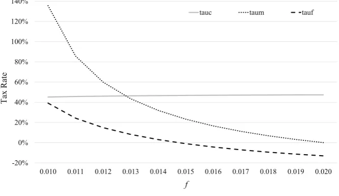
Now we turn to our main results. Figures1 and2 show how the optimal taxes τc, τm, τf change as the key parametersk, f change. Note thatτc, τm, τf are all of
the same order of magnitude, and the implied interest ratei, from the relationship (6), takes a sensible rate of values between 1 and 3% (not reported here).
In Fig.1,kvaries between 0 and 1, while f is fixed. This figure shows that first, bothτm, τf decrease markedly as the returns to scale in transactions costs increase,
thoughτm remains positive atk=1. Also, we see thatτmis consistently bigger than τm, consistent with Proposition1. We also see that forkabove 0.5 or so,τf becomes
a subsidy, a possibility that was shown theoretically in the previous section. We also
25 Output isy=1−l−s.
26 The precise calculation is as follows. The real value of consumption purchased using PAs is
c
1−j∗2
, and the real value of resources used in payments is f1−j∗.So, in the model, the cost of bank payment services as a share of consumption is f(1−j∗)
c
1−(j∗)2 = f
c(1+j∗).From Schmiedel
et al. (2012), and the discussion in the introduction, we estimate this to be to be about 3%. So, we set f
c(1+j∗) = 0.03.In our model, which calibrated to a consumption to GDP ratio of 0.7,c = 0.25 on average, and also alsoj∗is calibrated to 0.5. Substituting these elements into the last equation gives a value of f =0.011. This turns out to give rise to computational problems, and so we choose a slightly higher central value of f =0.015.
27 Matheny et al. (2016, p3) reports that “In 2015, cash remained the most frequently used retail payment
-20% 0% 20% 40% 60% 80% 100%
0.0 0.1 0.2 0.3 0.4 0.5 0.6 0.7 0.8 0.9 1.0
Tax Rate
k
tauc taum tauf
Fig. 1 Optimal tax rates askincreases. Note: In the figure, f = 0.019 rather than our central value of
f =0.015
-20% 0% 20% 40% 60% 80% 100% 120% 140%
0.010 0.011 0.012 0.013 0.014 0.015 0.016 0.017 0.018 0.019 0.020
Tax Rate
f
tauc taum tauf
Fig. 2 Optimal tax rates as f increases. Note: In the figure,k=1
see that real money balances should be taxed, τm > 0, even when k = 1. This is consistent with our theoretical finding in the previous section that the Correia-Teles result is not robust to alternative forms of payment. Finally, we see that both taxes are never zero at once, meaning that the use of cash and PAs is always distorted by the tax system, consistently with Proposition3.
In Fig.2, f varies between 0.01 and 0.02. This figure shows that both τm, τf
decrease markedly as the fee to scale in transactions costs increase, thoughτmremains
[image:21.439.54.389.54.244.2] [image:21.439.54.387.286.478.2]example, we see thatτmis consistently bigger thanτm, consistent with Proposition1. We also see that for f above 0.015 or so,τf becomes a subsidy, a possibility that was shown theoretically in the previous section. One intuition for whyτf can be negative can be gleaned from (A.3). As f rises, jt∗increases i.e. cash is used more, and this tends to make the effect of jt∗on the virtual leisure endowment,ej t positive. So, in
order to indirectly tax this virtual leisure endowment, jt∗should be reduced, which can be achieved by subsidizing PAs.
8 Conclusions
This paper has considered the optimal taxation of payment services, when realistically, the household can use either cash and or a bank account with services, such as debit cards, for the purchase of different varieties of goods. The setting is an extension of Correia and Teles (1996), to allow for the use of bank accounts as a form of payment, as in Freeman and Kydland (2000). Our first contribution is to develop simple formulae for the optimal ad valorem taxes on both real money balances and payment fees. For common specifications of the time transaction cost function, we can show that the tax on real money balances is always greater than the tax on fees, and also, while the former is always positive, the tax on fees may be negative.
Numerical results, using a calibrated version of the model, yielded additional insights. We found that both the inflation tax and the tax on fees decrease markedly as the returns to scale in transactions costs increase from zero to one. The results show also that both the inflation tax and the tax on fees increase as the bank fee decreases; this is interesting as the move away from cash is ultimately driven by technological innovation that reduces fees. Moreover, when the fee is large, the fee tax can be nega-tive, i.e. bank fees should be subsidized. We also find that the tax on bank fees, can be greater or less than the rate of consumption tax, although both taxes are of the same order of magnitude. So, our results show fairly robustly that this part of banking sector activity should probably not be left untaxed.
Appendix
Construction of the implementation constraint From (9)–(12) we have ,
χt =β tu
lt
λ , χtit
1+τtc
=βtult
λ (−smt) ,
χt
1+τtc
=βtuct
λ −χt
jt∗
2 sxt =β
tu ct
λ −
βtu lt
λ
jt∗
2 sxt,
χtf
1+τtf 1−jt∗=β
tu lt
λ sxt2ctjt∗
1−jt∗.
So, substituting these expressions in (8), we get:
∞
t=0 βt
ct
uct −ult
jt∗2sxt
−ultsmtmt +ultsxt2ctjt∗
1−jt∗
=∞
t=0 βt
ult(1−lt−st) . (A.1)
Rearranging (A.1) gives (14) as required.
Proof of Proposition1 Combining first-order conditions (11), (21) with 6, and (12) with (22), we get general formulae for the optimal taxes:
τm t =
μultemt
γ ξt , τ f t = −
μultej t
fξt .
(A.2)
Next, using using (A.2) and (17), we can computeet =(k−1)st−sxt2ctjt∗
1−jt∗
ej t =(1−k)sxtctjt∗−2sx xtct2
jt∗21− jt∗−sxtct
1−2jt∗,
to computeej t, we see that
τf t = −2μ
ult
fξt
(1−k)sxtctjt∗+2sx xtct2jt∗
2
1−jt∗+sxtct1−2jt∗
. (A.3)
Then, using the household optimization condition (12) to substitute out for f, we get
τf t 1+τtf =
μult
ξtsxtctjt∗
(1−k)sxtctjt∗+2sx xtct2jt∗
2
1−jt∗
+sxtct1−2jt∗
. (A.4)
Finally, simplifying the right-hand side of (A.4), and usingxt =(jt∗)ct, we get
τf t
1+τtf
=Z
1−k+1−2j ∗
t
jt∗
+2εxt
1−jt∗
jt∗
, εxt =
sx xtxt
sxt >0,