GraphM : an efficient storage system for high throughput of concurrent graph processing

warwick.ac.uk/lib-publications

Manuscript version: Author’s Accepted Manuscript

The version presented in WRAP is the author’s accepted manuscript and may differ from the

published version or Version of Record.

Persistent WRAP URL:

http://wrap.warwick.ac.uk/130159

How to cite:

Please refer to published version for the most recent bibliographic citation information.

If a published version is known of, the repository item page linked to above, will contain

details on accessing it.

Copyright and reuse:

The Warwick Research Archive Portal (WRAP) makes this work by researchers of the

University of Warwick available open access under the following conditions.

Copyright © and all moral rights to the version of the paper presented here belong to the

individual author(s) and/or other copyright owners. To the extent reasonable and

practicable the material made available in WRAP has been checked for eligibility before

being made available.

Copies of full items can be used for personal research or study, educational, or not-for-profit

purposes without prior permission or charge. Provided that the authors, title and full

bibliographic details are credited, a hyperlink and/or URL is given for the original metadata

page and the content is not changed in any way.

Publisher’s statement:

Please refer to the repository item page, publisher’s statement section, for further

information.

Concurrent Graph Processing

Jin Zhao

Huazhong University of Science and

Technology, China∗

zjin@hust.edu.cn

Yu Zhang

Huazhong University of Science and

Technology, China∗

zhyu@hust.edu.cn

Xiaofei Liao

Huazhong University of Science and

Technology, China∗

xfliao@hust.edu.cn

Ligang He

University of Warwick, United Kingdom

ligang.he@warwick.ac.uk

Bingsheng He

National University of Singapore, Singapore

hebs@comp.nus.edu.sg

Hai Jin

Huazhong University of Science and

Technology, China∗

hjin@hust.edu.cn

Haikun Liu

Huazhong University of Science and

Technology, China∗

hkliu@hust.edu.cn

Yicheng Chen

Huazhong University of Science and

Technology, China∗

yichengchen@hust.edu.cn

ABSTRACT

With the rapidly growing demand of graph processing in the real world, a large number of iterative graph processing jobs run concur-rently on the same underlying graph. However, the storage engines of existing graph processing frameworks are mainly designed for running an individual job. Our studies show that they are inef-ficient when running concurrent jobs due to the redundant data storage and access overhead. To cope with this issue, we develop an efficient storage system, called GraphM. It can be integrated into the existing graph processing systems to efficiently support concurrent iterative graph processing jobs for higher throughput by fully exploiting the similarities of the data accesses between these concurrent jobs. GraphM regularizes the traversing order of the graph partitions for concurrent graph processing jobs by streaming the partitions into the main memory and theLast-Level Cache(LLC) in a common order, and then processes the related jobs concurrently in a novel fine-grained synchronization. In this way, the concurrent jobs share the same graph structure data in the LLC/memory and also the data accesses to the graph, so as to amortize the storage consumption and the data access overhead. To demonstrate the efficiency of GraphM, we plug it into state-of-the-art graph processing systems, including GridGraph, GraphChi,

∗

Jin Zhao, Yu Zhang (Corresponding author), Xiaofei Liao, Hai Jin, Haikun Liu, and Yicheng Chen are with National Engineering Research Center for Big Data Technol-ogy and System, Services Computing TechnolTechnol-ogy and System Lab, Cluster and Grid Computing Lab, School of Computer Science and Technology, Huazhong University of Science and Technology, Wuhan, 430074, China.

Permission to make digital or hard copies of all or part of this work for personal or classroom use is granted without fee provided that copies are not made or distributed for profit or commercial advantage and that copies bear this notice and the full citation on the first page. Copyrights for components of this work owned by others than ACM must be honored. Abstracting with credit is permitted. To copy otherwise, or republish, to post on servers or to redistribute to lists, requires prior specific permission and/or a fee. Request permissions from permissions@acm.org.

SC ’19, November 17–22, 2019, Denver, CO, USA © 2019 Association for Computing Machinery. ACM ISBN 978-1-4503-6229-0/19/11. . . $15.00 https://doi.org/10.1145/3295500.3356143

PowerGraph, and Chaos. Experiments results show that GraphM improves the throughput by 1.73∼13 times.

CCS CONCEPTS

•Computer systems organization→Multicore architectures; •Information systems→Hierarchical storage management; • Computing methodologies→Parallel computing methodologies.

KEYWORDS

Iterative graph processing; concurrent jobs; storage system; data access similarity

ACM Reference Format:

Jin Zhao, Yu Zhang, Xiaofei Liao, Ligang He, Bingsheng He, Hai Jin, Haikun Liu, and Yicheng Chen. 2019. GraphM: An Efficient Storage System for

High Throughput of Concurrent Graph Processing. InProceedings of the

2019 International Conference for High Performance Computing, Networking, Storage, and Analysis (SC ’19), November 17–22, 2019, Denver, CO, USA.ACM, New York, NY, USA, 13 pages. https://doi.org/10.1145/3295500.3356143

1

INTRODUCTION

A massive number of concurrent iterative graph processing jobs are often executed on the same cloud platform, e.g., the Facebook Cloud [2] and the Huawei Cloud [3], to analyze their daily graph data for different products and services. For example, Facebook [2] adopts Apache Giraph [16] to support many different iterative graph algorithms (e.g., the variants of PageRank [29] and label propagation [8]) that are used by various applications running on the same underlying graph, e.g., social networks. However, existing solutions [13, 20–22, 25, 27, 37, 38] mainly focus on optimizing the processing of individual graph analysis jobs. In order to achieve the efficient execution of concurrent iterative graph processing jobs, the following two key challenges need to be addressed.

(a) Existing systems (b) Existing systems integrated with GraphM

Graph copy

Graph copy

Graph copy Memory

LLC

Memory LLC

Secondary storage

Graph data

Job-specific

data Job-specificdata Job-specific data Job-specific data Job-specific data Job-specific data

Data Access Synchronization. Runtime

Job 1 Job 2 Job 3 Job 1 Job 2 Job 3

Secondary storage

Graph data Graph

copy

Sharing & Dividing Plugin

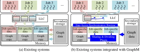
Figure 1: Execution of concurrent iterative graph process-ing jobs on (a) existprocess-ing graph processprocess-ing systems and (b) the ones integrated with GraphM

processing jobs usually traverse the same graph structure repeat-edly and a large proportion of the graph data accessed by them is actually the same. However, as shown in Figure 1 (a), with the graph storage engines highly-coupled with existing graph process-ing frameworks [13, 20, 22, 25], multiple copies of the shared graph data are maintained in theLast-Level Cache(LLC)/memory and are individually accessed by the concurrently running jobs. It results in inefficient use of data access channels and storage resources (e.g., the LLC/memory). There is a clear trend of running more and more iterative graph processing applications on the same platform. For example, DiDi [1] carries out more than 9 billion path planing [7] daily in 2017. The highly redundant overhead discussed above in-curs low throughput of concurrent iterative graph processing jobs. Second, diverse graph processing systems, which are highly cou-pled with their own storage engines, are developed, because it is important to employ suitable graph processing schemes for better performance according to their own requirements [26]. It is desired to decouple the graph storage system from graph processing to allow different graph processing systems to share a single opti-mized graph storage system, i.e., one storage system for all. Then, an optimized storage system can integrate with these graph pro-cessing engines to enable the concurrent and efficient execution of existing iterative graph processing applications while imposing little programming burden on the users.

To address these challenges, a novel and efficient storage sys-tem, calledGraphM, is proposed in this paper. It is a lightweight runtime system which can be run in any existing graph processing system and enables the system to support the concurrent execution of iterative graph processing jobs. In GraphM, we design a novel Share-Synchronizemechanism to fully exploit the similarities in data access between concurrently running jobs. The graph struc-ture data is decoupled from the job-specific data to be shared by multiple graph processing jobs, while only the job-specific data is maintained for each individual job. Then, GraphM regularizes the traversal paths of the graph partitions for the concurrent jobs by streaming the partitions into the LLC/memory in a common order and concurrently processing multiple jobs related to a common graph partition in novel fine-grained synchronization. Then, there is only a single copy of the graph structure data in the LLC/memory for multiple concurrent jobs, and the data access cost is amortized by them. More importantly, the existing graph processing systems residing above GraphM can still run with their own execution model, because the traversal path of the systems are regularized transparently in each iteration by GraphM. The idea is illustrated in Figure 1 (b), where only one copy of the common graph (rather

35 30 25 20 15 10 5 0

0 20 40 60 80 100 120 140 160

N

u

m

b

e

r

o

f

c

o

n

c

u

rr

e

n

t

jo

b

s

Times(hours)

Figure 2: Number of jobs traced on a social network

than several copies in the existing systems) is maintained to serve multiple concurrent jobs and the concurrent jobs can share the stor-age of the common graph and the data access to it. When writing the graph processing applications, the programmers only need to call a few APIs provided by GraphM to achieve higher performance for the concurrent execution of these applications. Moreover, in order to further improve the throughput, a scheduling strategy is designed in GraphM to specify the loading order of graph partitions to maximize the utilization ratio of the graph partitions loaded into the main memory.

This paper has the following main contributions:

• The redundant data access overhead is revealed when exist-ing graph processexist-ing system handles multiple concurrent jobs over a common graph, and the similarity between data accesses of the jobs is investigated.

• A novel and efficient storage system is developed to improve the throughput of existing graph processing systems for handling concurrent jobs while little programming burden is imposed on programmers.

• An efficient scheduling strategy is developed to fully exploit the similarities among the concurrent jobs.

• We integrate GraphM into existing popular graph process-ing systems, i.e., GridGraph [50], GraphChi [24], Power-Graph [14], and Chaos [32], and conduct extensive experi-ments. The results show that GraphM improves their perfor-mance by 1.73∼13 times.

The rest is organized as follows. Section 2 discusses our motiva-tion. GraphM is presented in Section 3 and the scheduling strategy is described in Section 4, followed by experimental evaluation in Section 5. The related work is surveyed in Section 6. This paper is concluded in Section 7.

2

BACKGROUND AND MOTIVATION

0 100 200 300 400 500 600

1 2 4 8

Number of concurrent jobs PageRank

WCC BFS SSSP

(d) Average execution time

0 2 4 6 8

1 2 4 8

M em o ry u sa g e (G B )

Number of concurrent jobs Pagerank

WCC BFS SSSP

(a) Total memory usage 0

2 4 6 8

1 2 4 8

M em o ry u sa g e (G B)

Number of concurrent jobs Pagerank

WCC BFS SSSP

(a) Total memory usage

0 20 40 60 80 100 120

1 2 4 8

L L C m is se s (Bi ll io n s)

Number of concurrent jobs PageRank

WCC BFS SSSP

(b) Total last-level cache misses

0.006 0.007 0.008 0.009 0.010

1 2 4 8

N

um

be

r

of L

P

I

Number of concurrent jobs

(c) Average number of LPI

PageRank WCC BFS SSSP E xe cut ion t im e (S ec onds )

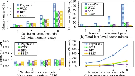
Figure 3: Performance evaluation of concurrent iterative graph processing jobs executed on GridGraph

2.1

Redundant Data Access Overhead

With the storage engines highly-coupled with existing graph pro-cessing systems [13, 20, 22, 25], the common graph is individually accessed by concurrent iterative graph processing jobs. It generates excessive unnecessary overhead in storage resource and data access channel, and thus significantly increases the data access cost. This eventually results in low system throughput because the data access cost usually dominates the total execution time of iterative graph processing [36]. To demonstrate it, we evaluated the performance of concurrent jobs on GridGraph [50] over Twitter [23], where the platform is the same as that introduced in Section 5.

We observe that more data access cost is generated with the increase of the number of concurrent jobs. It is because that mul-tiple copies of the common underlying graph are loaded into the storage by its storage engine for the concurrent jobs. For example, as depicted in Figure 3(a), the total amount of memory usage for the processing of each partition significantly increases due to re-dundant memory usage as the number of jobs increases. Figure 3(b) describes the total number of LLC misses for different number of concurrent graph processing jobs over GridGraph [50], which rep-resents the size of the graph data loaded into the LLC. It can be seen that much redundant graph data is also swapped into the LLC. In addition, with more concurrent jobs, more serious contention for storage resources and data access channels occurs in a resource-limited machine, thereby causing more page faults, LLC misses, etc. As shown in Figure 3(c), the average number ofLLC misses per Instruction(LPI) increases when more concurrent jobs are executed over GridGraph [50], due to the intense cache interference caused by the fact that multiple copies of the same graph partition are being individually loaded into the LLC. For example, when there are eight concurrent jobs, the average number of the LPI of these jobs increases by about 10% comparing with that of one job, because the graph data required for the execution of the instructions of different jobs is usually the same for these concurrent jobs. It exacerbates the above challenges. To show the impact of resource contention, Figure 3(d) shows the average execution time of each job as the number of jobs increases. It can be observed that the execution time of each job significantly increases as the number of jobs increases.

2.2

Our Motivation

Figure 4(a) depicts the percentage of the graphs that are shared by different number of concurrent jobs traced from a social network,

60 70 80 90 100

1 2 3 4 5 6

Time (hours) (a) Percentage of shared graph

#>1 #>2 #>4 #>8 0 20 40 60 80 100 120

1 2 4 8

N u m b er o f L P I

Number of concurrent jobs PageRank

WCC BFS SSSP

(b) Average number of LPI

0 20 40 60 80 100 120

1 2 4 8

L L C m is se s (Bi ll io n s)

Number of concurrent jobs PageRank

WCC BFS SSSP

(b) Total last-level cache misses

P e rc e n ta g e sh a re d b y # jo b s (% ) 5 6 7 8 9

1 2 3 4 5 6

A v era g e d at a ac ce ss t im es

Time (hours)

(b) Average data access times

Figure 4: Information traced on the social network

and Figure 4(b) indicates the average number of accessed times of the graph partitions which have been repeatedly accessed by different jobs in each time period (one hour). It can be observed from Figure 4 that there are strong similarities between the data accesses of many concurrent jobs, because the same graph is repeatedly traversed by them.

Observation 1. Most proportion of the same graph is shared by multiple concurrent jobs during the traversals, which is called the spatial similarity.As shown in Figure 4(a), more than 82% of the same underlying graph is concurrently processed by the concurrent jobs during the traversals. Unfortunately, in most existing systems, the intersection of the graph data handled by the concurrent jobs is not shared in the LLC/memory, and it is accessed by these jobs along different graph paths individually, which results in a large amount of redundant data access overhead. Ideally, it only needs to maintain a single copy of the same graph data in the LLC/memory to serve the concurrent jobs in each traversal.

Observation 2. The same graph data may be accessed by different concurrent jobs over a period of time, which is called the temporal similarity.In detail, since the same underlying graph is individu-ally handled by the concurrent jobs, the shared graph data may be frequently accessed by multiple jobs within their repeated traver-sals (about 7 times on average as shown in Figure 4(b)). However, the existing systems are not aware of this temporal similarity, so that the graph data frequently accessed by different jobs may be swapped out of the LLC/memory, which leads to the rise of the data access cost. Therefore, the accesses to the shared graph data for the concurrent jobs should be consolidated so that the same graph data is only loaded into the LLC/memory once to be handled by the concurrent jobs in each traversal for once.

The strong spatial and temporal similarities motivate us to de-sign a storage system, which can integrate with existing graph processing engines to manage the data accesses of concurrent iter-ative graph processing jobs for higher throughput while imposing little programming burden on the users.

3

OVERVIEW OF GRAPHM

Graph processing job queue

CPU cores

Original graph data

Chunk tables

Secondary storage Chunk

tables Memory

LLC

Synchronizing Profiling

Chunk 1

GraphM Architecture

Load

Suspended job

Profiled job Unprofiled job

Control flow Data flow

Executable ones

Suspended ones

Load

② ③ ④

①

Graph Partition

Chunk 1 Chunk 2 Chunk 3 Chunk 4

②

Graph Partition

Chunk 1 Chunk 2 Chunk 3 Chunk 4

Graph partition

Chunk 1 Chunk 2 Chunk 3 Chunk 4

Specific graph representation

Graph preprocessor Graph sharing controller

Sy

nc

hr

oni

za

ti

on

m

a

na

ge

r

Chunk 1Chunk 1

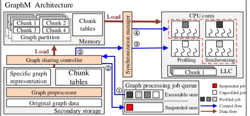
Figure 5: System architecture of GraphM

3.1

System Architecture

Generally, the data needed by an iterative graph processing job is composed of the graph structure data (i.e., the graph represented byG=(V,E,W)), job-specific data (e.g., ranking scores for PageR-ank [29], and the componentIDfor Connected Components [19]), marked asS. During the execution, each job needs to update its Sthrough traversing the graph structure data until the calculated results converge. Specifically, in existing systems [12, 24, 44, 50], GandS are stored separately. GraphM enablesGto be shared by the concurrent jobs, thereby fully exploiting the strong spa-tial and temporal similarities between these jobs. Figure 5 shows the architecture of GraphM. It consists of three main components: graph preprocessor, graph sharing controller, and synchronization manager, which are overviewed in the following subsections.

Graph Preprocessor.The graph formats and the preprocessing methods can be different for various graph processing systems. Thus, before the graph processing, the original graph stored in GraphM needs to be converted to the graph representation format specific to the graph processing system (which needs to handle this graph) using user defined functionConvert(). For example, the orig-inal graph data is converted to the grid format for GridGraph [50], the shard format for GraphChi [24], the CSR/CSC format for Pow-erGraph [14], and the edge list format for Chaos [32]. After that, as existing graph processing systems [12, 24, 44, 50], the graph is divided into partitions for parallel processing and the operations of the concurrent jobs are still performed on the specific graph rep-resentation of the related system. Meanwhile, the graph structure partitions are further logically divided and labelled as a series of chunks according to the common traversing order of the graph of the jobs for the purpose of fine-grained synchronization as the following described. In addition, it can exploit the cache locality because the chunks can be fit in the LLC. When dividing a partition, achunk_tablearray is generated to describe the key information of each logical chunk for the purpose of regular accessing of the graph partition shared by multiple jobs, where the specific graph representation is not modified.

Graph Sharing Controller.After graph preprocessing, the specific graph structure data needs to be loaded into the memory to serve concurrent jobs. This functional module is used to assign the loading order and also load the graph structure partitions, which will be shared by concurrent jobs. The module is designed as a thin API to be plugged into the existing graph processing systems. The API can be expressed as:P_ji←Sharinд(G,Load()).Gis the name of the graph to be loaded and is used to identify the range of shared memory

Table 1: GraphM Programming Interface

APIs Description

Init() Initialization of GraphM

GetActiveV ertices() Get active vertices in each iteration

Sharinд() Load the shared graph data

Start()/Barrier() Notify GraphM to start or end

fine-grained synchronization

which contains the shared graph structure partition.Load()is the original load operation of the graph processing system integrated with GraphM for the loading of graph data, andPi_jdenotes a loaded graph structure partitionPi shared by thejthjob. When the jobs need to be concurrently executed (the step○1), the loaded graph structure data is only shared by active jobs, while inactive jobs are suspended and wait for their active graph vertices/edges to be loaded into the memory (the step○2). In addition, the mutations and updates of the shared graph structure data are isolated among concurrent jobs to ensure the correctness of the processing. In this way, only one copy of the shared graph structure data needs to be loaded and maintained in the memory to serve concurrent jobs. Thus, the redundant cost of the memory resource and the amount of disk data transfers are reduced.

Synchronization Manager.When the graph structure partition is shared by concurrent jobs, it is individually accessed by them in a consistent logical order according to its programming model. However, since some jobs may skip the inactive vertices for them and the computational complexity of the processing of the streamed data is usually different for various jobs, these jobs may process the shared graph partitions in different orders. Hence, the shared graph data is irregularly streamed into the LLC by concurrent jobs, resulting in unnecessary data access cost. To solve this problem, we use a novel and efficient fine-grained synchronization way to fully exploit the temporal similarity between these jobs.

This module enables the chunks of the shared graph data to be regularly streamed into the LLC by traversing the same graph path in fine-grained synchronization. In detail, each job needs to be profiled to determine the computational load of each chunk before each iteration (the step○3). The computing resources are then unevenly allocated to the jobs for their concurrent execution based on the skewed computational load of these jobs (the step○4), so as to synchronize the graph traversals with low cost. By such means, each chunk typically only needs to be loaded into the LLC once and be reused by concurrent jobs in each iteration. Thus, it significantly reduces the data access cost by fully exploiting the similarities of these jobs.

Programming APIs.To invoke GraphM in graph analysis pro-grams, the user only needs to insert our APIs shown in Table 1 into existing graph processing systems. Note that it does not need to change the graph applications above these graph processing sys-tems. In detail,Init()is used to initialize GraphM by preprocessing the graph as described in Section 3.Sharing()function is inserted in existing graph processing systems to replace the original data load operation for the efficient load of the shared graph data. Note that the parameter in the functionSharing()is various for different graph processing systems, e.g., the parameter is the functionLoad()

GraphM.Init() /*Initialization of GraphM*/ StreamEdges(){

… /*Setup the active partitions*/

GraphM.GetActiveVertices() for(each active partition){

partition GraphM.Sharing(G, load()) /*Notify GraphM to start synchronization*/

GraphM.Start() for(each edge  partition) … /*Process the streamed edges*/

/*Notify GraphM to end synchronization*/

GraphM.Barrier() }

}

/*Edge streaming function in GridGraph*/ StreamEdges(){

… /*Setup the active partitions*/

for(each active partition){ /* The original data load operation*/

partition  load() for(each edge  partition) … /*Process the streamed edges*/

} }

(a) Pseudocode of GridGraph (b) Pseudocode of GridGraph integrated with GraphM

Figure 6: An example to illustrate how to integrate GraphM into existing graph processing system

Meanwhile, two notification functions (i.e.,Start()andBarrier()) are inserted at the beginning and the end of the procedure that traverses the shared graph structure partition for the graph pro-cessing systems, respectively. Note thatGetActiveVertices()is also provided to get the active vertices before each iteration, because some graph processing systems (e.g., GridGraph [50]) allow to use this operation to skip the processing of inactive vertices. Figure 6 takes GridGraph [50] as an example to show how to integrate exist-ing graph processexist-ing systems with GraphM to efficiently support concurrent graph processing jobs, whereLoad() is the graph loading operation of GridGraph [50].

3.2

Graph Preprocessing

The CPU utilization ratio and the cache locality may be influenced by the chunk size, denoted bySc. Setting it too large may increase the data access cost. This is because when only a part of a chunk can be loaded into the LLC, this part has to be swapped out when the rest of the chuck is loaded into the LLC. Since a chunk will be accessed by different concurrent jobs, the part of the chunk that has been swapped out has to be loaded into the LLC again, which increases the overhead. On the contrary, setting the chunk size too small may lead to frequent synchronization among the concurrent jobs that are processing this chunk since only when concurrent jobs have finished processing this chuck can they move to process the next one.

The suitable chunk sizeScis determined in the following way. Ndenotes the number of CPU cores, andCLLCdenotes the size of the LLC.Scis set to be such a maximum integer that satisfies Formula 1, whereSGis the size of the graph data,|V|is the number of vertices in the graph,Uvis the data size of each vertex, andris the size of the reserved space in the LLC. The first term on the right of the formula represents the LLC size required to accommodate the chunks which are concurrently processed by the threads of a running job (the number of threads usually equals to the number of CPU cores in the computer, hence we haveSc×N). The second term represents the size required to store the job-specific data in the LLC. Note that the size of a chunk is also a common multiple of the size of an edge and the size of a cache line for better locality.

Sc×N+Sc×N

SG × |V| ×Uv+r ≤CLLC (1)

With this setting, the same chunk only needs to be loaded into the LLC once and is then reused by all concurrent jobs with low synchronization cost. Only the job-specific data need to be replaced by different jobs, where the jobs are triggered to handle the loaded data in a round-robin way.

Note that the graph is not physically divided into the chunks of the size discussed above. Rather, in the preprocessing phase, the

Algorithm 1Partition Labelling Algorithm

1: functionLabel(Pi,Setci)

2: edдe_num←0

3: c_table←null

4: foreach edgee∈Pi do

5: ifes ∈c_tablethen

6: c_table.N+(es)←c_table.N+(es) + 1

7: else

8: c_table.InsertEntry(⟨e_s,1⟩)

9: end if

10: /*Count the number of edges labelled inc_table*/

edдe_num←edдe_num+ 1

11: ifedдe_num×S_|EG_| ≥ScorPiis visitedthen 12: Set_ci.Store(c_table)

13: /*Prepare to store information of next chunk*/

Clear(c_table,edдe_num)

14: end if

15: end for 16: end function

graph is traversed so that each graph partition is labelled as a series of chunks in the order in which the graph data is streamed into the LLC. The labelling information of each chunk is stored in a key-value table, calledchunk_table. Each entry of thechunk_table is a key-value pair, in which the key is the ID of a source vertex in the chunk (denoted byv) and the value is the number of this vertex’s outgoing edges in the chunk (denoted byN+(v)).

Algorithm 1 shows how to label a partition, e.g.,Pi. When an edge is traversed,N+(v) of the edge’s source vertex (i.e.,es) is incremented by one in the corresponding entry ofchunk_table(i.e.,

c_table) (Line 6). If the source vertex of the edge is not found in

c_table, a new entry (i.e., a key-value pair) is created with the value being 1 and inserted into the table (Line 8). When the number of edges inc_tablemakes the chunk size to be the value determined by Formula 1 or all edges ofPi are visited (Line 11), these edges are treated as a chunk and thec_tableis stored as an element of an array, i.e.,Set_ci (it holds the information of all chunks inPi) (Line 12).c_tableis then cleared and used to store the information of the next labelled chunk, where the value ofedдe_numis reset to zero (Line 13). Note that this procedure only runs once for a graph processing system, although it incurs extra cost.

3.3

Memory Sharing of Graph Structure

Algorithm 2Graph Sharing Algorithm

1: functionSharing(G, Load()) /*Triggered by jobj*/

2: /*Get an active partitionPi that needs be loaded*/

Pi _{←GetActivePartition()}

3: /*Get the set of jobs that need to handlePi*/

Ji _←GetJobs(Pi₎

4: Resume(Ji) /*Resume the suspended jobs inJi*/

5: ifj<Jithen/*jdoes not need to handlePi*/

6: Suspend(j) /*Suspend the jobj*/

7: end if

8: ifPi is not in the memorythen 9: /*Create a shared buffer to storePi*/

Bu f ←CreateMemory(G,Pi)

10: Bu f ←Load(Pi) /*LoadPi intoBu f*/

11: else/*JobjgetsPiin the shared buffer*/

12: Bu f ←Attach(G) /*AttachBu f toj*/

13: end if

14: Remove(j,Ji) /*RemovejfromJi*/

15: returnBu f 16: end function

IDs (PIDs) of the active jobs of the corresponding graph partition. Each job needs to update the global table in real time. Particularly, the order of the entries in the global table is determined by the loading order of their corresponding graph partitions by default. After that, a lightweight API (i.e., the functionSharinд() described in Algorithm 2) is designed to extend the graph loading operation in the existing systems, allowing the job (e.g., the jobj) to share the loaded graph partitions.

In detail, when the jobj calls the functionSharinд(), it first gets theIDof an active partitionPiassigned by GraphM (Line 2), where the loading order of the partitions to be loaded is assigned by GraphM along the order of their corresponding entries in the global table. The set of jobs (e.g.,Ji) that need to handlePi are then obtained from the global table (Line 3). After that, the active jobs recorded inJi are popped fromsuspended_queueand their executions are resumed (Line 4), if these jobs are suspended. If the current jobj is not inJi (i.e.,j does not need to handlePi), it is suspended to release its computing resources for the execution of the jobs that need to handlePi, and is pushed intosuspended_queue (Lines 5-7). IfPiis not in the shared memory, a bufferBu f is created to store it (Lines 9-10). Otherwise, the jobjis assigned to share the loaded graph partitionPiin the memory with the other concurrent jobs (Line 12). Then, the PIDs of the jobj is removed from the

Ji (Line 14) and the jobjbegins to handle the graph partitionPi referenced by the returned results (Line 15).

3.3.2 Ensuring of Consistent Snapshots.The shared graph may be updated or mutated by some jobs over time, resulting in incorrect results or runtime errors. Hence, a storage management technique is further designed to ensure the consistency of snapshots among the concurrent jobs.

When the shared graph structure data needs to be modified, e.g., removing or adding edges/vertices, users need to call our API to handle the evolving graph. In detail, GraphM first copies the cor-responding chunks of the graph data that need to be modified to

Phys ical address Virtual address _{of Job 2}

Shared memory Mutation 2

Chunk 1

Virtual address of Job 1

copy copy

low high

Graph St ructure of Job 1

Shared Graph St ructure

Updat e 3

Graph St ructure of Job 2

Copy 3 _{Chunk 4}

Mutation 2

Chunk 4 Chunk 3 Chunk 2

Chunk 1 Chunk 4

Updat e 3

Chunk 2 Chunk 1

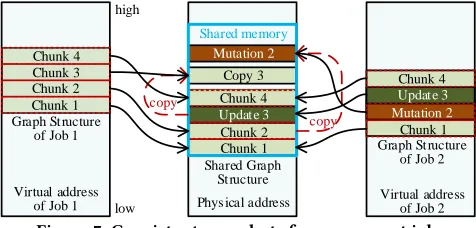
Figure 7: Consistent snapshots for concurrent jobs

other shared memory space. If it is mutated by a job, the modifica-tion will be applied to the copied chunks, and alter the mapping of the virtual address of the corresponding chunks in the job to the copied chunks. Thus, the shared graph structure is not changed, it can be shared by other jobs. Besides, the copied chunks will be released when the corresponding job is finished. Different from graph mutation, which is only visible to its corresponding job, the graph update is only available to the jobs submitted after the update. Therefore, the shared graph structure will be updated to serve the newly submitted jobs, and previous jobs can refer to the copied chunks to continue their calculation. Note that when all previous jobs are completed, these copied chunks will be released. By do-ing so, the shared graph structure is always visible and shared by the newly submitted jobs. Note thatSet_ci also needs to be updated accordingly when the shared graph is updated.

As shown in Figure 7, two jobs are submitted, wherejob1 is submitted beforejob2. If a graph update arrives after the submission ofjob1, it will create a copy (e.g.,copy3) for the corresponding graph structure data (e.g.,chunk3) forjob1 to use, andchunk3 is going to be updated. Besides, the copied data will be released when

job1 is finished. Then, a new graph structure chunk (i.e.,update3) is constructed beforejob2 is submitted. Ifjob2 needs to modify a chunk (e.g.,copy2) of the graph structure, the mutation is applied to the copied data to generatemutation2, which is only visible tojob2. Note that the graph mutations and updates usually only happen to a small fraction of graph data, and thus a majority of the graph structure data can be shared by concurrent jobs and the update cost of theSet_ci is also small.

3.4

Fine-grained Synchronization for Regular

Streaming

This section discusses the details of the fine-grained synchroniza-tion way for efficient execusynchroniza-tion of concurrent jobs.

3.4.1 Mining the Similarities between Concurrent Jobs.This fine-grained synchronization scheme mines the chunks of the shared graph that can be concurrently handled by the jobs in each iteration. Moreover, the similarities are dynamically changed because the vertices in the chunks may be activated or converged in some jobs during the iteration, which therefore needs to be dynamically updated before each iteration.

procured by tracing the change of vertices states after each itera-tion. In general, a vertex needs to be processed within the current iteration only when its value has been updated by the neighbours within the previous iteration. Note that the active vertices in the first iteration are designated by the user for each job. To express the active vertices succinctly, a bitmap is created for each job. If some jobs do not skip the useless streaming, all of their vertices are active by default. Then, the active chunks of concurrent jobs can be obtained by their bitmaps and thechunk_tablearrays. Finally, the similarities between the data accesses of the concurrent jobs can be rapidly obtained based on the intersection of their active chunks. 3.4.2 Fine-grained Synchronization of Traversals. To fully exploit the temporal similarity between the data access of the concurrent jobs, it enables the chunks loaded into the LLC to be processed by these jobs in a regular way. In detail, the computing resources are unevenly allocated to the concurrent jobs to synchronize their data accesses, because the computational loads of different jobs are usually skewed when processing each chunk. Generally, the load of each jobj for a chunk is determined not only by the amount of edges that need to be processed, but also by the computational complexity of the edge processing function of this job, denoted asT(Fj). In addition, the average data access time for each edge, indicated asT(E), affects the execution time of the jobs. Thus, for each job, the fine-grained synchronization has two phases, i.e., the profiling phase and the syncing phase.

Profiling Phase.This phase is to profile the needed information (i.e., T(Fj) and T(E)) of the jobs. When a new job (e.g., the jobj) is submitted, the profiling phase of this job traverses the shared graph partition (e.g.,Pi) and captures its execution time, denoted byT_ji, which is composed of the graph processing time and the graph data access time. Thus,T_jiis represented as the following formula:

T(F_j) × Õ

k∈Ci Õ

v∈V_k∩Aj N_k+(v)+

T(E) × Õ

k∈Ci Õ

v∈V_k

N_k+(v)=T_ji

(2)

whereCiis the set of chunks in the partitionPi, andVkis the set of vertices in thekthchunk.Ajis the set of active vertices for the job

jwithin the current iteration, which can be easily obtained via its bitmap.N_k+(v)is the number of out-going edges of the vertexvin thekthchunk.VkandN_k+(v)are stored in the correspondingSetci. According to Formula 2, after the processing of the first two active partitions of each jobj, the needed information, i.e.,T(F_j)andT(E), of the jobjcan be obtained, whereT(E)_{is a constant for the same}

graph and only needs to be profiled once for different jobs. Syncing Phase.After obtainingT(F_j)of the concurrent jobs, the computational load of the jobs in each chunk is easily acquired before each iteration. In detail, the computational load of thejth job for the processing thekthchunk (i.e.,Lk_j) can be determined by the following equation:

Lk_j =T(Fj) × Õ

v∈V_k∩Aj

N_k+(v) (3)

Each partition may be handled by the threads of different con-current jobs. To achieve fine-grained synchronization and better locality, the threads of different jobs handling the same partition need to be migrated to the same CPU core to synchronize their

Partition 2 Partition 3

Job 1 Partition 1 Partition 4

Partition 3 Partition 1 Partition 4 Partition 2

iteration x iteration x+1

iteration y

Job 2

Suspended

Suspended

Resumed

1 1/2 1/3 1/3

Pri(P)

Partition 1 Partition 2

Job 1 Partition 3 Partition 4

Partition 2 Partition 3 Partition 4 Partition 1

iteration x

iteration y

Job 2

Suspended Suspended

Resumed

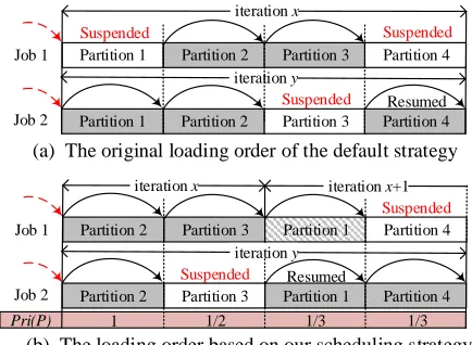
(a) The original loading order of the default strategy

(b) The loading order based on our scheduling strategy

Suspended

Figure 8: An example to illustrate the scheduling of loading order of graph partitions, wherepartition1is activated by the other partitions ofjob1and can be handled at the(x+1)th

iteration forjob1

data access by scheduling their CPU time slices. Usually, only a small amount of migrations are generated, because these threads access a series of chunks synchronously each time in the partition. After that, the computing resources need to be allocated unevenly to the threads of the concurrent jobs according to the skewed com-putational load. Each thread monopolizes the CPU time to finish processing the current chunk. Apparently, the execution time of the chunk for each thread can be represented by its corresponding computational loadaccording to Formula 3, except the thread that first processes the chunk. It is because that the graph data needs to be loaded into the LLC by this thread and its execution timeF_jkfor

thekthchunk can be obtained by the following equation:

Fk_j =Lk_j +T(E) × Õ

v∈V_k

N_k+(v) (4)

After the corresponding execution times of all threads have elapsed, the jobs will process the next chunk concurrently with the reallocated computing resources.

4

THE SCHEDULING STRATEGY FOR

OUT-OF-CORE GRAPH ANALYSIS

The loading order of graph partitions in the out-of-core graph pro-cessing systems may cause the similarities between the data access of concurrent jobs not to be fully exploited due to the following reasons. First, some jobs may only need to handle a few of parti-tions in the current iteration, but more partiparti-tions will be activated in the next iteration. For example, in BFS [11] and SSSP [28] only one or a few vertices are active at the beginning, but then a large number of vertices will be activated by these vertices. Second, the activated partitions may be accessed by other jobs in the current iteration, e.g., PageRank [29] and WCC [35]. Hence, a partition may be repeatedly loaded into the memory to serve different jobs in contiguous iterations, resulting inefficient usage of the partitions that are loaded into the memory.

Table 2: Graph datasets used in the experiments

Datasets Vertices Edges Data sizes LiveJ [5] 4.8 M 69 M 526 MB Orkut [5] 3.1 M 117.2 M 894 MB Twitter [23] 41.7 M 1.5 B 10.9 GB UK-union [9] 133.6 M 5.5 B 40.1 GB Clueweb12 [4] 978.4 M 42.6 B 317 GB

with the least number of active partitions. Other partitions may be activated in these jobs, which can then advance to next iteration to process the activated partitions, as shown in Figure 8. In this way, the strategy enables the partitions loaded into the memory to serve more concurrent jobs, further amortizing the data access cost, especially when the size of the graph is very large.

To achieve the goal described above, each partition is assigned a priority. The partitions with the higher priority are loaded first into the memory to serve the related jobs, so that these jobs can complete current iteration as quickly as possible to activate other partitions. Two rules are applied when setting the priority. First, the partitions are given a higher priority when they are handled by the jobs with fewer active partitions. Second, a partition is given the highest priority when it is processed by most jobs. In summary, the priorityPri(Pi)of each partitionPiis set using Equation 5, where

Jidenotes the set of jobs to handlePi in the next iteration,Nj(P) denotes the number of active partitions of thejthjob (i.e., a job of the setJi), andN(Ji)denotes the number of jobs in the setJi.

Pri(Pi)=MAX_j∈Ji 1 Nj(P)×N(J

i_{) (5)}

The values ofNj(P) andN(Ji)are directly obtained from the global table. The priority is calculated before each complete tra-versal over all the partitions. After that, the entries in the global table are sorted according to the priority of their corresponding partitions and determine the loading order of the partitions. From Figure 8, we can observe that the partition 1 can serve more con-current jobs when it has been loaded into the memory via this scheduling strategy. Then, the similarities between concurrent jobs are fully exploited.

5

EXPERIMENTAL EVALUATION

5.1

Experimental Setup

The experiments are conducted on a server with two 8-core Intel Xeon E5-2670 CPUs (each CPU has 20 MB last-level cache) operating at the clock frequency of 2.6 GHz, a 32 GB memory and a 1 TB hard drive, running Linux kernel 2.6.32. All codes are compiled with cmake version 3.11.0 and gcc version 4.9.4. Table 2 shows the properties of the five real-world graphs used in our experiments, where LiveJ, Orkut, and Twitter can be stored in the memory, while the size of UK-union and Clueweb12 are larger than the memory size. Four representative graph processing algorithms are used as benchmarks, includingweakly connected component(WCC) [35], PageRank [29],single source shortest path(SSSP) [28],breadth-first search(BFS) [11]. These algorithms have different characteristics in the data access and resource usage. For example, PageRank and WCC are network-intensive [40], which need to frequently traverse the majority of the graph structure, whereas SSSP and BFS only traverse a small fraction of the graph at the beginning.

Table 3: Preprocessing time (in seconds) LiveJ Orkut Twitter UK-union Clueweb12 GridGraph 20.89 35.07 439.59 2,312.11 19,267.28 GridGraph-M 21.86 35.76 463.65 2,681.04 22,401.90

To evaluate the performance, we submit WCC, PageRank, SSSP, and BFS in turn in a sequential or concurrent manner until the specific number of jobs are generated, where the parameters are randomly set for different jobs although these jobs may be the same graph algorithm. In detail, the damping factor is randomly set by a value between 0.1 and 0.85 for each PageRank job. The root vertices are randomly selected for the BFS jobs and the SSSP jobs. The total number of iterations is a randomly selected integer between one and the maximum number of iterations for each WCC job. For the concurrent manner, the time interval between successive two submissions follows the poisson distribution [15] withλ=16 by default. All benchmarks are run for ten times and the experimental results are the average value.

To evaluate the advantages of GraphM, we integrate GridGraph [50] with GraphM (calledGridGraph-Min the experiments) to run multi-ple concurrent graph processing jobs. We then compare GridGraph-Mwith two execution schemes of the original GridGraph, called GridGraph-SandGridGraph-C.GridGraph-Ssequentially processes the jobs, whileGridGraph-Cconcurrently handles the jobs (but each job runs independently without sharing the underlying graph struc-ture data as inGridGraph-M). InGridGraph-C, the concurrent jobs are managed by the operating system. We choose GridGraph [50] since it is a state-of-the-art one and outperforms other out-of-core graph processing systems [24, 33].

In addition, we also finally integrate GraphM into the other popu-lar systems (i.e., GraphChi [24], PowerGraph [14], and Chaos [32]) and evaluate their performance. There, Eigen (version 3.2.10) is needed by GraphChi. OpenMPI (version 2.1.6), boost (version 1.53.0), zookeeper (version 3.5.1), bzip2 (version 1.0.6), gperftools (version 2.0), hadoop (version 1.0.1), and libevebt (version 2.0.18) are required by PowerGraph. Boost (version 1.53.0) and zmq (version 4.3.1) are needed by Chaos. The experiments of PowerGraph and Chaos are done on a cluster with 128 nodes, which is connected via 1-Gigabit Ethernet. Each node is the same as the above described. Because PowerGraph and Chaos may not get the best performance due to high communication cost when all nodes are used to handle all jobs for some graphs, the nodes are divided into groups and each group of nodes are used to handle a subset of jobs so as to make the jobs executed over PowerGraph and Chaos in a high throughput mode, where the newly submitted jobs are assigned to the groups in turn. Note that, when some jobs need to be executed on Power-Graph/Chaos over a group of nodes, the graph is only loaded into the distributed shared memory consisting of the memory of this group of nodes. In the experiments, for high throughput of 64 jobs over LiveJ, Orkut, Twitter, UK-union, and Clueweb12, the suitable number of groups is set to 8, 8, 4, 1, 1 for PowerGraph and 8, 4, 2, 1, 1 for Chaos, respectively.

5.2

Preprocessing Cost

L i v e J O r k u t T w i t t e r U K - u n i o n C l u e w e b 0 . 0

0 . 2 0 . 4 0 . 6 0 . 8 1 . 0 1 . 2 1 . 4 1 . 6 1 . 8

N o rm al iz ed e x ec u ti o n t im e

D a t a s e t s

G r i d G r a p h - S G r i d G r a p h - C G r i d G r a p h - M

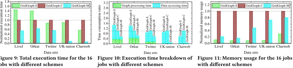
Figure 9: Total execution time for the 16 jobs with different schemes

L i v e J O r k u t T w i t t e r U K - u n i o n C l u e w e b 0 . 0

0 . 4 0 . 8 1 . 2 1 . 6 2 . 0 2 . 4 2 . 8 3 . 2

G ri d G ra p h -M G ri d G ra p h -C T im e co n su m p ti o n r at io

D a t a s e t s

G r a p h p r o c e s s i n g t i m e D a t a a c c e s s i n g t i m e

G ri d G ra p h -S G ri d G ra p h -S G ri d G ra p h -C G ri d G ra p h -M G ri d G ra p h -S G ri d G ra p h -C G ri d G ra p h -M G ri d G ra p h -S G ri d G ra p h -C G ri d G ra p h -M G ri d G ra p h -S G ri d G ra p h -C G ri d G ra p h -M

Figure 10: Execution time breakdown of jobs with different schemes

L i v e J O r k u t T w i t t e r U K - u n i o n C l u e w e b 0 . 0

0 . 2 0 . 4 0 . 6 0 . 8 1 . 0 1 . 2

N o rm al iz ed m em o ry u sa g e

D a t a s e t s

G r i d G r a p h - S G r i d G r a p h - C G r i d G r a p h - M

Figure 11: Memory usage for the 16 jobs with different schemes

of graph is larger than the memory size, the labelling procedure of the graph increases the preprocessing time by an average of 16.1%, because these graph needs to be reloaded into the memory. When the graph can be stored in the memory, the labelling procedure of the graph only increases the preprocessing time by an average of 4%. As evaluated, the extra storage cost of GraphM is also small and occupies 5.5%-19.2% of the space overhead of the original graph, i.e., 70.6 MB (13.4%), 49.2 MB (5.5%), 2.09 GB (19.2%), 4.5 GB (11.2%), and 19.9 GB (6.3%) for LiveJ, Orkut, Twitter, UK-union, and Clueweb12, respectively. In general, when the graph has larger maximum out-degree and lower average out-out-degree, the ratio of its extra space overhead to the space overhead of the original graph is higher. It is because that the vertices with larger out-degree have more replicas stored in different chunks and the extra space overhead is also usually proportional to the ratio of the number of vertices to the number of edges. For example, the maximum out-degree and the average out-degree are 2,997,469 and 35 for Twitter, respectively, while they are 7,447 and 48 for Clueweb12, respectively. Thus, the space overhead ratio of Twitter is higher than that of Clueweb12. Note that, although GraphM needs such extra space overhead, more storage overhead can be spared by GraphM because only one copy of the graph structure data (instead of multiple copies) needs to be maintained by existing systems for multiple jobs when they are integrated with GraphM.

5.3

Overall Performance Comparison

Figure 9 shows the total execution time of 16 concurrent jobs with different schemes. It can be observed that GridGraph-M achieves shorter execution time (thus higher throughput) than the other two schemes for all graphs. Comparing with GridGraph-S and GridGraph-C, GridGraph-M improves the throughput by about 2.6 times and 1.73 times on average respectively when the graphs can be stored in the memory, and by 11.6 times and 13 times on average respectively in the case of out-of-core processing. The throughput improvement is achieved for the lower data access cost in GridGraph-M.

To evaluate data access cost, we further break down the total exe-cution time in Figure 10. It can be observed from this figure that less graph data accessing time is required in GridGraph-M compared with the other two schemes, especially when the size of the graph is very large. For example, for UK-union, the data accessing time is reduced by 11.48 times and 13.06 times in GridGraph-M in com-parison with GridGraph-S and GridGraph-C. The reasons for the lower data access cost of GraphM are two-fold:1)only a single copy of the same graph data needs to be loaded and maintained in the

memory to serve the concurrent jobs, reducing the consumption of memory and disk bandwidth and the intense resource contention; 2)the graph data is regularly streamed into the LLC to be reused by the jobs, which avoids unnecessary memory data transfer by reducing LLC miss rate and minimizes the volume of data swapped into the LLC.

Figure 11 shows the usage of main memory during the execution. As observed, M consumes less memory than GridGraph-C, but more than GridGraph-S. This is because the graph structure data is shared in the memory for concurrent jobs by GraphM (thus GridGraph-M consumes less memory than GridGraph-C), and the job-specific data of all concurrent jobs as well as thechunk_tableof the loaded graph data is loaded into the memory at the same time (thus GridGraph-M consumes more memory than GridGraph-S). Note that as the number of vertices in the graph increases, the job-specific data for concurrent jobs need more memory resource. For example, the memory usage of GridGraph-M over UK-union is 8.2 times bigger than that of GridGraph-S because the job-specific data of the 16 jobs is stored in the memory. However, it is still only 71% of the memory usage of GridGraph-C. Hence, the memory resource is efficiently utilized in GraphM since redundant memory consumption regarding the common graph data is eliminated.

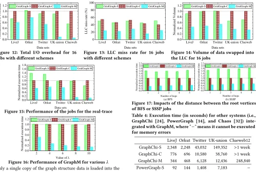
In Figure 12, we evaluate the total I/O overhead of these 16 jobs over three schemes. As observed, the I/O overhead is significantly reduced in GridGraph-M when the size of the graph data is larger than the memory size. It is because that the same graph data only needs to be loaded into the memory once in each iteration for concurrent jobs. However, when the graph can be fitted in the memory, there is no much difference in the I/O overhead among these three schemes, since this graph is cached in the memory via memory mapping and only needs to be read from disks once. Thus, GraphM brings better performance improvement for the out-of-core graph processing for less I/O cost. More specifically, when processing UK-union, the I/O overhead is reduced by 9.2 times and 10.1 times compared with GridGraph-S and GridGraph-C. In addition, GridGraph-C usually performs more I/O operations than GridGraph-S, because there is intense contention for using the memory resource among the jobs, which causes the graph data to be swapped out of the memory.

L i v e J O r k u t T w i t t e r U K - u n i o n C l u e w e b 0 . 0

0 . 2 0 . 4 0 . 6 0 . 8 1 . 0 1 . 2

N

o

rm

al

iz

ed

I

/O

o

v

er

h

ea

d

D a t a s e t s

G r i d G r a p h - S G r i d G r a p h - C G r i d G r a p h - M

Figure 12: Total I/O overhead for 16 jobs with different schemes

L i v e J O r k u t T w i t t e r U K - u n i o n C l u e w e b

0

2 0 4 0 6 0 8 0 1 0 0

L

L

C

m

is

s

ra

te

(

%

)

D a t a s e t s

G r i d G r a p h - S G r i d G r a p h - C G r i d G r a p h - M

Figure 13: LLC miss rate for 16 jobs with different schemes

L i v e J O r k u t T w i t t e r U K - u n i o n C l u e w e b 0 . 0

0 . 2 0 . 4 0 . 6 0 . 8 1 . 0 1 . 2

N

o

rm

al

iz

ed

V

o

lu

m

e

D a t a s e t s

G r i d G r a p h - S G r i d G r a p h - C G r i d G r a p h - M

Figure 14: Volume of data swapped into the LLC for 16 jobs

LiveJ Orkut Twitter UK-union Clueweb 0.0

0.2 0.4 0.6 0.8 1.0 1.2 1.4 1.6 1.8

Normaliz

ed exe

cuti

on time

Data sets

GridGraph-S GridGraph-C GridGraph-M

Figure 15: Performance of the jobs for the real-trace

2 4 6 8 10 0.0

0.2 0.4 0.6 0.8 1.0 1.2

Normaliz

ed exe

cuti

on time

Value of 

GridGraph-S GridGraph-C GridGraph-M

Figure 16: Performance of GraphM for variousλ only a single copy of the graph structure data is loaded into the LLC and the access to this data is shared by the jobs. The graph structure data loaded into the LLC can serve more concurrent jobs in GridGraph-M, resulting in better data locality for these jobs.

Moreover, we traced the total amount of data swapped into the LLC for these 16 jobs. Generally, GridGraph-C needs to swap a larger amount of graph data into the LLC than GridGraph-S, because there is more redundant memory data transfer caused by the intense cache interference among concurrent jobs. As shown in Figure 14, when processing UK-union, the amount of data swapped into the LLC in GridGraph-S is 65% of GridGraph-C. Nevertheless, we observe that the amount of swapped data in GridGraph-M is still much less than GridGraph-S (e.g., only 55% for UK-union). This is because the data access similarities among concurrent jobs are fully exploited by GraphM.

We also evaluate the performance of GraphM via submitting the jobs according to the real trace shown in Figure 2, where different number of jobs are submitted at various point of time according to the real trace. In Figure 15, the results show that GridGraph-M improves the throughputs of GridGraph-S and GridGraph-C by 1.5–7.1 times, and 1.48–9.8 times, respectively, for the real trace, because of lower graph storage overhead and less data access cost. In addition, we evaluate the impacts of job submission frequency on GraphM over UK-union in Figure 16 by using different value ofλ. The results show that higher speedup is obtained by GraphM when the jobs is more frequently submitted (i.e., largerλ). Figure 17 shows the performance of 16 BFS or SSSP jobs with randomly selected root vertices within the range of different number of hops over LiveJ.

(a) BFS (b) SSSP

1 2 3 4 5

0.0 0.2 0.4 0.6 0.8 1.0 1.2 1.4 1.6 1.8 2.0 2.2

Normaliz

ed exe

cuti

on time

Number of hops

GridGraph-S GridGraph-C GridGraph-M

1 2 3 4 5

0.0 0.2 0.4 0.6 0.8 1.0 1.2 1.4 1.6 1.8 2.0 2.2

Normaliz

ed exe

cuti

on time

Number of hops

GridGraph-S GridGraph-C GridGraph-M

Figure 17: Impacts of the distance between the root vertices of BFS or SSSP jobs

Table 4: Execution time (in seconds) for other systems (i.e., GraphChi [24], PowerGraph [14], and Chaos [32]) inte-grated with GraphM, where“−”means it cannot be executed for memory errors

LiveJ Orkut Twitter UK-union Clueweb12 GraphChi-S 2,348 2,248 43,032 149,352 >1 week GraphChi-C 776 696 10,580 38,760 >1 week GraphChi-M 344 468 6,128 12,436 248,840 PowerGraph-S 92 144 1,408 7,183 −

PowerGraph-C 83 111 1,153 6,653 −

PowerGraph-M 43 75 795 3,820 −

Chaos-S 224 159 4,668 29,538 487,272 Chaos-C 516 588 12,011 30,943 >1 week Chaos-M 121 106 2,261 10,614 156,881

We find that higher speedup is achieved by GraphM for stronger spatial/temporal similarities of the data accesses when the root vertices of the BFS or SSSP jobs are closer to each other.

5.4

Performance of Scheduling Strategy

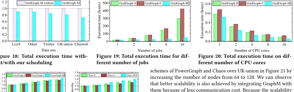
We also evaluate the impacts of our scheduling strategy on the performance of GraphM when it is integrated with GridGraph. M and M-without are the versions of GridGraph-M with our scheduling strategy (Section 4) and without our sched-uling strategy, respectively. In Figure 18, we traced the total execu-tion time of the above 16 jobs on GridGraph-M and GridGraph-M-without. We can observe that GridGraph-M always outperforms GridGraph-M-without. The execution time of GridGraph-M is only 72.5% of GridGraph-M-without over Clueweb12. It is because the graph partitions loaded into the memory can serve as many con-current jobs as possible, minimizing the data access cost.

5.5

Integration with Other Systems

L i v e J O r k u t T w i t t e r U K - u n i o n C l u e w e b 0 . 0

0 . 2 0 . 4 0 . 6 0 . 8 1 . 0 1 . 2

N

o

rm

al

iz

ed

e

x

ec

u

ti

o

n

t

im

e

D a t a s e t s

G r i d G r a p h - M - w i t h o u t G r i d G r a p h - M

Figure 18: Total execution time with-out/with our scheduling

1 2 4 8 1 6

0

1 0 0 2 0 0 3 0 0 4 0 0 5 0 0

E

x

ec

u

ti

o

n

t

im

e

(h

o

u

rs

)

N u m b e r o f j o b s

G r i d G r a p h - S G r i d G r a p h - C G r i d G r a p h - M

Figure 19: Total execution time for dif-ferent number of jobs

1 2 4 8 1 6 0 . 0

0 . 2 0 . 4 0 . 6 0 . 8

E

x

ec

u

ti

o

n

t

im

e

(h

o

u

rs

)

N u m b e r o f C P U c o r e s G r i d G r a p h - S G r i d G r a p h - C G r i d G r a p h - M

Figure 20: Total execution time on dif-ferent number of CPU cores

(a) PowerGraph (b) Chaos

64 80 96 102 128 0.0

0.2 0.4 0.6 0.8 1.0 1.2 1.4 1.6

Speedup

Number of nodes

PowerGraph-S PowerGraph-C PowerGraph-M

64 80 96 102 128 0.0

0.2 0.4 0.6 0.8 1.0 1.2 1.4 1.6 1.8

Speedup

Number of nodes

Chaos-S Chaos-C Chaos-M

Figure 21: Scalability of different distributed schemes

as described in Section 5.1. We can observe that all systems get better speedups after integrating GraphM into them. Diverse graph processing systems get various performance improvements after using GraphM, because the ratios of the graph access time to the total execution time are different for them. In general, when the ratio of data access time to the execution time is higher for the original system, the greater performance improvement is gotten by GraphM via reducing the redundant graph structure data storage overhead and access cost.

5.6

Scalability of GraphM

Figure 19 shows the performance of various number of concurrent PageRank jobs on different schemes of GridGraph over Clueweb12. Better performance improvement is achieved by GraphM when the number of jobs increases. GridGraph-M gets speedups of 1.79, 3.04, 4.92, and 5.94 against GridGraph-S when the number of jobs is 2, 4, 8, and 16, respectively. It is because that more data access and stor-age cost is spared by GraphM through amortizing it, as the number of jobs increased. Note that the fine-grained synchronization oper-ation of GraphM does not occur when there is only one job, and thus there is no much difference in the execution time among the three schemes at this moment. The synchronization cost occupies 7.1%–14.6% of the total execution time of the job on GraphM for our tested instances. In addition, as the contention for resources (e.g., memory and bandwidth) gets more serious, the performance of GridGraph-C becomes much worse than that of GridGraph-M, even GridGraph-S. Thus, simply adopting existing graph processing systems to support concurrent jobs may be a terrible choice.

We then evaluate the scaling out performance of GraphM. For this goal, we first evaluate the execution time of 16 jobs on different schemes of GridGraph for Twitter on a single PC by increasing the number of CPU cores. From Figure 20, we find that GridGraph-M performs better than other ones under any circumstances, especially when the number of cores is more, because the storage and access of the graph structure data is shared by the concurrent jobs in GridGraph-M, while the other schemes have a higher data access cost. Second, we evaluate the performance of 64 jobs on different

schemes of PowerGraph and Chaos over UK-union in Figure 21 by increasing the number of nodes from 64 to 128. We can observe that better scalability is also achieved by integrating GraphM with them because of less communication cost. Because the scalability of GraphM is greatly decent in most situations, we believe it can efficiently support concurrent graph processing in industry.

6

RELATED WORK

Recently, many graph processing systems have been proposed. GraphChi [24] and X-Stream [33] achieve efficient out-of-core graph processing through sequentially accessing storage. Hao et al. [39] keep frequently accessed data locally to minimize the cache miss rate. TurboGraph [18] fully exploits the parallelism of multi-core and FlashSSD to overlap CPU computation and I/O operation. FlashGraph [49] adopts a semi-external memory graph engine to achieve high IOPS and parallelism. PathGraph [41] designs a path-centric method to acquire better locality. By using the novel grid for-mat and the streaming-apply model, GridGraph [50] improves the locality and reduces I/O operations. HotGraph [44], FBSGraph [45], DGraph [47], and DiGraph [46] accelerate graph processing via faster state propagation. However, these systems mainly focus on optimizing individual graph processing, which lead to redundant storage consumption and data access cost as handling multiple con-current graph processing on same graph. Hence, Seraph [40] tries to decouple the data model and computing logics for less consump-tion of memory. CGraph [43, 48] proposes to reduce the redundant data accesses in the concurrent jobs. Nevertheless, they are tightly coupled to their own programming models and graph processing engines, which cause re-engineering burden of various applica-tions for users while using these engines. Compared with them, GraphM transparently improves the throughput of concurrent jobs on existing graph processing systems.