Misfolding dominates protein evolution

PROTEIN EVOLUTION

Thesis by

David Allan Drummond

In Partial Fulfillment of the Requirements for the Degree of

Doctor of Philosophy

CALIFORNIA INSTITUTE OF TECHNOLOGY

Pasadena, California 2006

© 2006

Having worked for some stellar managers, I know just how lucky I am to work for Frances Arnold. She makes science fun. Frances has shaped my development as a scientist in ways great and small, some direct (her ability to cut to an issue’s heart, and to explain how to make an idea matter, continue to amaze me) and some by example (she delivered insightful comments on complex manuscripts within days at most, even at the very nadir of her chemotherapy). I am so grateful for her blind investment in me, an older student with no publications, no lab experience, and no knowledge of protein biophysics when I entered her lab in 2003. I’ve tried to rise to the standard she sets, and imagine that I will keep trying for the rest of my scientific lifetime.

I am indebted to Claus Wilke on innumerable levels. Without Claus’s intelligence, gentle suggestions, brutal judgments, and old-fashioned hard labor, most of the results reported here would never have existed. He has been a generous and calm mentor, a joy to work for, and then with, on the considerable corpus we’ve generated, P-value by R-script, in four years. As described in Chapter 4, it was his idea to use principal component regression, and his analysis on yeast, that created the main result reported there. He wrote the first versions (and in my view the most difficult parts) of the lattice protein simulations that became Chapter 6. Claus’s influence on me is impossible to overstate; he taught me most of what I know about the gory details of doing science day-to-day, from the difference between thinking I have a result and actually having it, down to the Benjamini-Hochberg false-discovery-rate correction for multiple tests. I envy the students who will get him at 22 instead of 30.

end, his influence on this thesis is, as he might say, “completely obvious!”

Discussions with Jesse Bloom have been invaluable: his elegant work on protein mutational tolerance provides the backdrop for Part 1 of this thesis, and his analysis of evolutionary rates inspired Part 2. Michelle Meyer taught me how to think like an experimentalist (my failure to become one cannot be laid at her competent feet!) and has been a wonderful sounding-board for ideas. Conversations with Zhen-Gang Wang built my confidence in theory work, and he provided critical guidance on certain mathematical treatments, particularly for the simple models in Chapters 1 and 3 (errors in conception and execution are solely mine).

Joff Silberg performed the experiments analyzed and modeled in Chapter 3 and helped develop the ideas presented there. Jeff Endelman, and indeed most members of the Arnold Lab, engaged in countless impromptu back-and-forth sessions that greatly improved the ideas here. George Georgiou and Brent Iverson at the University of Texas were generous with their experimental data and insight, and Chapter 2 was the result; Alpan Raval did eye-wateringly thorough work on the failings of partial correlation analyses; and Brian Baer supported my sometimes greedy (Chapter 6!) use of the Alice computing cluster resources at Michigan State University. Alice Sogomonian, Divina Bautista and Mariah Oh helped keep this creaky old vessel in fighting trim. All have my thanks.

The distinguished members of my thesis committee (Frances, Chris, Erik Winfree, Michael Elowitz and Shuki Bruck) provided just the right amount of guidance and were always available when I had questions. By providing me with an NIH Training Grant, the CNS option let me do whatever I pleased for my first three years, including going to work for a chemical engineer unaffiliated with the option.

Acknowledgments ...iii

Abstract...vi

Table of Contents ...viii

List of Figures and Tables ...ix

Preface ...12

Part 1: Misfolding Dominates Directed Protein Evolution...15

Chapter 1: Balancing diversity and misfolding to find improved proteins ...16

Chapter 2: Coupling in high-error-rate random mutagenesis...38

Chapter 3: On the conservative nature of intragenic recombination ...70

Part 2: Misfolding Dominates Natural Protein Evolution...99

Chapter 4: A single dominant constraint on protein evolution...100

Chapter 5: The translational robustness hypothesis ...123

Chapter 6: Misfolding dominates genome evolution ...149

Table 1.1: Correlation analysis of folded-mutant fitness properties on the likelihood of improved function. ... 33 Figure 1.1: Overview of lattice protein properties... 34 Figure 1.2: A simple Markov-chain model for the probability of protein improvement .... 36 Figure 1.3: Simulation results for the probability of improving lattice protein stability... 37 Table 2.1: scFv antibody mutational results and corresponding predictions for PCR and

Poisson-distributed mutations ... 61 Table 2.2: Mutational spectra for libraries... 62 Table 2.3: Comparison of retention of wildtype digoxigenin binding for scFv antibody

libraries with analytical predictions ... 63 Figure 2.1: Mutational distributions for two high-error-rate scFv antibody libraries

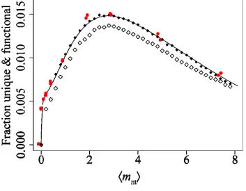
compared with Poisson and PCR distributions ... 64 Figure 2.2: Equation 2.3 explains previously reported experimental results ... 65 Figure 2.3: Error-prone PCR error rates strongly influence the fraction of unique and

functional sequences ... 66 Figure 2.4: The requirement for uniqueness reduces effective library size and leads to

library- and protocol-dependent optimal library mutation rates ... 67 Figure 2.S1: Comparison of Equation 2.3 to simulation results... 68 Figure 2.S2: Simulation results match predictions for number of unique, functional

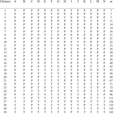
proteins... 69 Table 3.S1. Functional PSE-4/TEM-1 chimeras... 91 Table 3.S2. Characteristics of PSE-4 mutant libraries... 92 Table 3.S3: Values of neutrality ν and recombinational tolerance ρ for lattice protein

Figure 3.2: Lattice protein results mirror experimental findings... 96 Figure 3.3: Neutrality ν is correlated with recombinational tolerance ρ for lattice proteins

... 97 Figure 3.4: Chimeras occupy a functionally enriched ridge in sequence space ... 98 Table 4.1: Partial correlation analysis of seven putative determinants of evolutionary rate

... 120 Figure 4.1: Principal component regression on the rate of protein evolution (dN) in 568

yeast genes reveals a single dominant underlying component... 121 Figure 4.2: Principal component regression on the rate of synonymous-site evolution (dS)

in 568 yeast genes reveals a single dominant underlying component ... 122 Table 5.1: Evolutionary rate vs. expression correlations (Kendall’s τ) relative to four yeast

species for S. cerevisiae genes, including and excluding preferred codons ... 142 Table 5.S1: Evolutionary rate vs. CAI correlations (Kendall’s τ) relative to four yeast

species for S. cerevisiae genes, including and excluding preferred codons ... 143 Table 5.S2: Significant asymmetries in synonymous codon usage between high- and

low-expressed paralogs at aligned positions reflects relative adaptedness ... 144 Figure 5.1. Expression level governs gene and paralog evolutionary rates in S. cerevisiae

... 145 Figure 5.2. Phylogenetic relationships between analyzed yeast species ... 146 Figure 5.3. Translational selection against the cost of misfolded proteins can act at two

distinct points ... 147 Figure 5.S1. Estimating expression level with the codon adaptation index (CAI) reveals

reproduces multiple sequence evolution trends from yeast ... 170 Figure 6.3. All ten pairwise correlations between dN, dS, dN/dS, Fop and expression level

in S. cerevisiae and a simulated genome are similar... 171 Figure 6.4. Why highly expressed model proteins evolved slowly... 172 Figure 6.5: Sequence conservation patterns in simulated genes reflect structural constraints and differ with expression level ... 174 Figure 6.6: Intragenic nonsynonymous-synonymous correlations predicted from

simulation results are present and numerically similar in yeast... 175 Figure 6.S1: Estimates of translation outcomes based on the translational error spectrum

PREFACE

Happy families are all alike; every unhappy family is unhappy in its own way.

Leo Tolstoy, Anna Karenina

Functional proteins are all alike; every misfolded protein is misfolded in its own way. An array of powerful techniques may be swiveled with delight in the direction of a functional protein. There are the countless stereotypical biophysical assays: visualization of circular dichroism and tryptophan fluorescence and NMR spectra, denaturation with heat or chaotropic agents, crystallization, separation by charge and solubility. Biological interrogations may also commence to determine such properties as activities, pathway participation, and subcellular localization. The very existence of huge protein databases with fixed schema attests to the Tolstoyesque alikeness of functional proteins; indeed, as in families of either temperament, protein family members correlate in their behavior down to the very angle of their backbones.

database of bridge collapses or train derailments. Unhappy families may make great novels, but misfolded proteins make ghastly research subjects.

Such is the view as we pan the camera across basic and applied biology, from biochemistry to biophysics to genetics to protein engineering, and it persists as genomics and evolution enter the frame. The panorama of data is focused through the lens of functionality: catalytic residues, active sites, binding domains, structural motifs, conformational changes, macromolecular complexes, interactome network diagrams. In the genomic era, few annotations are more intriguing than “conserved protein of unknown function.”

Yet we continue to grapple unhappily with the unpleasant reality that while functional proteins might be (in some senses) all alike, most protein functions are different. Worse, in the absence of similar sequences with known properties, we cannot reliably predict or engineer the folding or function of a protein. We cannot even reliably predict if or how a single mutation will alter protein fold or function, except to say that the results (like the predictions) probably won’t be pretty.

Averaging over all such mutations, though, we might predict two basic outcomes: minimal change, or misfolding-induced loss of function. Such averaging consistently arises in the repeated protein-engineering experiments (by nature or by humans) that generate huge ensembles by the conserved processes of mutation and recombination: the differences dilute out, and the similarities remain. In any genome-wide trend, function dilutes out. In any general directed evolution strategy, function dilutes out. And as it does, misfolding titrates in.

Misfolded proteins are all alike; every functional protein is functional in its own way. #

powerful effect protein misfolding exerts over optimal mutation rates. Chapter 2 is a detective story in mutagenesis that attempts to explain why the popular method of error-prone PCR mutagenesis, when run at very high mutation rates, seems to produce a startling excess of functional and improved proteins relative to expectations (such as those set in Chapter 1). Chapter 3 compares high-error-rate mutagenesis to protein recombination for the exploration of distant regions of protein sequences space, and provides a simple model for why random mutants lose function at rates up to 16 orders of magnitude higher than chimeric proteins with the same number of amino acid substitutions.

Throughout Part 1, I focus on understanding mutational tolerance in proteins. Intuition suggests that the rate at which proteins evolve in nature should be related to their mutational tolerance. In Part 2, I analyze the natural evolution of proteins.

PART 1

C h a p t e r 1

BALANCING DIVERSITY AND MISFOLDING TO FIND IMPROVED PROTEINS

I begin with a block of marble and chip away the parts that are not statue. Attributed to Michelangelo Buonarroti

Proteins have evolved to perform an unreasonable number of functions under very reasonable conditions. At room temperature, in water, often with high activity and low toxicity, proteins can be expected to cleave sugar (hexokinase), fix carbon (Rubisco), convert ion gradients into propulsion (flagellar motors), bind oxygen (hemoglobin), cut DNA (restriction enzymes), cut other proteins (proteases), and recognize invaders (antibodies). Yet these sleek, efficient nanomachines turn finicky, balky or useless when aimed at tasks we humans find useful1, even such related tasks as cutting other DNA2 or recognizing other invaders3.

The diversity of protein functions makes these molecules an equally seductive and daunting engineering target. Given that we cannot yet assign a structure to an amino acid sequence with any reliability, and cannot assign functions to structures without an evolutionary cheat-sheet, how can we hope to engineer these molecules?

Such a shift may seem positively Faustian: we may obtain engineering results, but only by forfeiting our scientific soul, the imperative to understand why. But such a tradeoff is illusory. We have merely shifted problem domains, trading the presently intractable deterministic challenge of designing an improved protein for the (possibly) more tractable probabilistic challenge of designing an ensemble likely to contain such a sequence.

In protein engineering, such ensembles are called libraries4, and typically they grow, like a small-town branch, from one or a handful of ragged donations, wild-type proteins which in their human usefulness are not bestsellers, but have some promising bits. Most libraries are mutant libraries, in which the variants differ by a few characters. Some are recombination libraries, in which entire folios have been promiscuously swapped around. Whatever the method of generating a library, the goal at the end is to check out of it a better book than we donated—a tall order. Like books, most randomly fiddled-with proteins aren’t just bad proteins, they are nonsensical garbage. Rational library design4-6 seeks general ways to increase our likelihood of finding better proteins, which (in a theme elaborated below and in the following two chapters) often simply involves seeking to minimize the time spent sorting garbage.

A central principle that allows evolutionary library design to be an engineering discipline rather than an anecdotal craft is that, to perform any of their myriad functions, proteins must fold. Sequences encoding folded proteins are exceedingly rare in the space of all possible sequences,1,7 so the search for folded proteins necessarily guides the search for functional and improved proteins. Most mutations that disrupt function also disrupt folding.8-11 (Recently, this observation’s converse has been examined for one family of enzymes: 94–96% of mutant cytochromes P450 that retained fold also retained at least half the wild-type activity on a target substrate12.)

required to obtain improvement, we must better understand the tradeoff between folding and diversity.

For the rest of this chapter, I develop intuition about the interplay of folding and diversity in a specific class of mutant libraries, develop a simple mathematical treatment of this interplay (elements of which are expanded in the following two chapters), present a protein folding model exercised throughout this thesis, compare model and simulation results for the problem of obtaining mutants with increased stability, and raise questions to be addressed in Chapters 2 and 3.

Modeling improvement, and the Principle of Pessimistic Additivity

Let us assume we can assign a fitness w, a performance rating, to every mutant. We will begin with a wild-type sequence s having fitness w₀. The wild type may itself be an engineered mutant; “wild type” and “starting point” will be used interchangeably here. The objective is to isolate an improved mutant having some unspecified number of amino-acid substitutions (mutations) m whose fitness exceeds a threshold w_t >w₀. I will assume such improvement requires proper folding, where the folding state f is encoded by a binary random variable taking values 1 (true) and 0 (false). The probability of improvement in a folded protein having m amino-acid mutations generated from a starting sequence s I will denote Pr(w>w_t f =1,m,s).

details of mutagenesis but for the moment honors the possibility that the distribution may depend on the wild type’s sequence composition.

Some mutations may disrupt protein function, often by destabilizing the native structure enough to cause misfolding.11 The probability of mutation-induced misfolding depends on the wild type (because more-stable proteins can tolerate a wider array of destabilizing effects)11 and the number of mutations (because stability changes are roughly additive)13. Recognizing this dependence, I will denote the probability of proper folding given m mutations applied to a wildtype sequence Pr(f =1m,s).

These definitions lead to a straightforward formulation of the probability that a library starting from a wild-type sequence s contains an improved mutant:

) Pr( ) , 1 Pr( ) , , 1 Pr(

)

Pr(w w s w w f m s f m s ms

m t

t = > = =

>

∑

where the sum over the number of mutations m runs from zero to the length of the protein, and there is no sum over f because the probability of improvement in a misfolded mutant is zero.

m

s m f =1 , )≈ν

Pr( (1.2)

where the parameter ν, the neutrality, represents the probability that a mutation to a folded protein yields another folded protein. Neutrality describes the average connectivity of the neutral network of folded sequences,18 hence its name, and it is determined by the protein structure and minimal stability requirement shared by all such sequences.11,19 With

)

Pr(ms and Pr(f =1m,s) in hand, we are left with only the probability )

, , 1

Pr(w>w_t f = m s , the probability of improvement given a folded mutant separated from wildtype by m mutations.

Progression past this point requires some knowledge (or, more often, an assumption) about how mutations affect fitness. A common assumption implicitly made in most directed protein evolution experiments is that mutations are roughly additive. Directed evolution is the sequential improvement of protein properties using iterated rounds of mutagenesis and selection, a physical realization of an adaptive walk in protein sequence space.1 Such adaptive walks have been exhaustively studied elsewhere,20 and a central result holds that when mutations have strongly coupled (non-additive) effects, the fitness landscape becomes so rugged and decorrelated that most adaptive walks rapidly terminate at sub-optimal local maxima: you take a short walk up a small hill to nowhere. That stepwise directed evolution is so widely used suggests that practitioners are willing to assume mutations are not strongly coupled; that such evolution has produced so many successes suggests they are right to do so.

Additivity confers pleasant mathematical properties which allow the potentially daunting probability of improvement Pr(w>w_t f =1,m,s) to be treated simply. Many mutational effects on highly complex properties are roughly additive,13 and virtually any property can be treated additively over small enough ranges.

directing evolution which must encompass the widest range of wild types, a weaker but more palatable (albeit lighthearted) principle might be substituted:

The Principle of Pessimistic Additivity

A directed evolution strategy that will not work assuming additive mutational effects will not work at all.

To the extent we assume anything about multiple mutations, we choose additivity over hopelessness, and even then, we do not expect any mutations to be precisely additive. (In this sense, the assumption of additivity parallels the common statistical assumption of normality, with similar attendant caveats.)

My touchstone question is: “Suppose mutations affected my target property roughly additively. How should I direct evolution?”

Directed evolution with additive fitness, given folded mutants

The question, “How should I direct evolution?” may be phrased more tactically: “To increase the probability of finding improved mutants, under what conditions should I increase the mutation level of my library?”

My aim in all that follows is to examine the role of protein misfolding in decisions about mutagenesis. Accordingly, I adopt a rather minimalist and intuitive approach here and relegate detailed quantitative analyses to a specific practical problem in Chapter 2.

Suppose misfolding is not a concern, or we restrict our attention to those mutants which retain fold. Further suppose that libraries in which every sequence has the same number of mutations m may be constructed. When should m be increased?

Guiding intuitions

Such a question may seem impossible to answer, because the wild-type sequence may have idiosyncratic properties. However, the sequence space for a typical protein, while the size of a multi-universe, has the geography of Mayberry: very little is more than several steps away, and the whole lot may be traversed end-to-end in a few hundred mutational paces1. As a result, applying a only handful of mutations to any wild-type sequence without disrupting folding will yield an ensemble of mutants in which, on average, all idiosyncrasies have vanished. Further mutations will tend to generate ensembles with identical properties. A clear example of this behavior is found when looking at the fraction of mutants retaining wild-type fold as a function of mutational distance m: after roughly four amino acid changes, the effects of initial wild-type stability have given way to the average properties associated with the protein structure shared by all mutants.11,14 As a result, an additive model linking mutation-induced stability changes to the probability of folding can be replaced with a simple mean-field model with little accuracy loss.14

the average fitness of a folded protein in sequence space be w. If the wildtype sequence has w₀ ≈w, then mutations which preserve folding will also tend to preserve the starting point for future attempts at improvement. If the wildtype has w₀ <w, then directed evolution is easy: most folded mutants will have higher fitness. If, however, the wild-type sequence has w₀ >w, then each mutation reduces fitness on average, moving the goalposts farther and farther away.

In a library, the behavior of the mean fitness of a folded protein is rarely crucial, because for any problem requiring real effort, the asymptotic average fitness w will be below the desired fitness. The potential value of multiple additive mutations lies in the behavior of the variance. For any sum of independent random variables, the variance increases with the number of summands. Thus, if the mean fitness hovers in place (w₀ ≈w), again restricting our attention to folded proteins, more independent additive mutations are better on average. If the mean fitness tends upward (w₀ <w), more mutations are even better.

If w₀ >w, then an additional mutation makes sense only if the increase in variance compensates for the expected fitness reduction. As mutations accumulate and the mean recedes, only those mutational combinations far out on the positive tail have any hope of exceeding the threshold for improvement. A single deleterious mutation can erase all the small positive gains in a stroke, because when w₀ >w, the average deleterious effect will tend to be larger than the average beneficial effect.

On the basis of this intuitive treatment, considering the mean and variance of fitnesses of folded mutants, I predict that the mean will predict improvement better when w₀ <w (less-fit than average wild type) than when w₀ >w, and the mean plus the variance will always predict improvement better than the mean.

Quantitative model

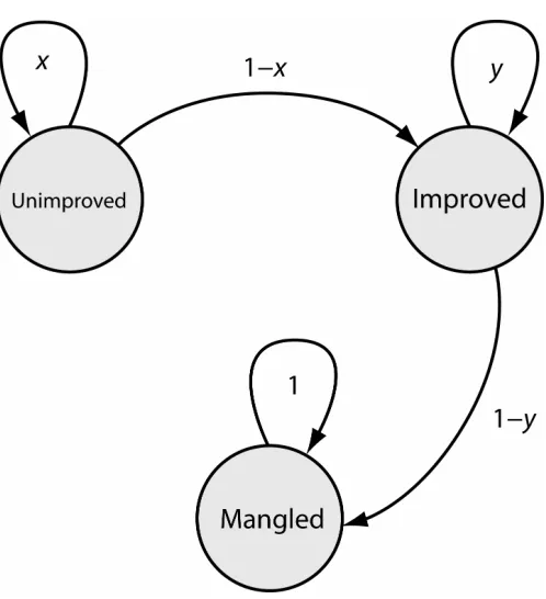
A full mathematical treatment is beyond my scope, but a simple model to capture the battle between beneficial and deleterious mutations may be constructed as follows. Suppose that, within the network of folded proteins, there exists a sub-network of improved proteins which are above some threshold of additive fitness. Starting from an unimproved wild-type protein, mutations represent a random walk which occasionally ends on an improved protein. In some cases, an otherwise improved protein might suffer a virtually unrecoverable deleterious mutation, and I will call such proteins “mangled.” (The assumption of irreversibility reflects the presumption that the distribution of fitness changes will be strongly skewed toward deleteriousness, such that an average deleterious mutation can only be compensated by several beneficial mutations, leading to an effectively unrecoverable fitness deficit.) Let the transition probability from one unimproved protein to another be x, from a folded protein to an improved protein be 1−x, from one improved protein to another be y, and from an improved to a mangled protein be 1−y (Figure 1.2). Then our system is equivalent to a three-state Markov chain, containing states “improved”, “unimproved”, and “mangled,” with:

initial state vector

⎥ ⎥ ⎥ ⎥ ⎦ ⎤ ⎢ ⎢ ⎢ ⎢ ⎣ ⎡ = 0 1 0

v and transition matrix

⎥ ⎥ ⎥ ⎦ ⎤ ⎢ ⎢ ⎢ ⎣ ⎡ − − = 1 0 1 0 0 0 1 y x x y A .

(

)

m _{y x}

y x

x m

unimp

imp _⎟⎟ −

⎠ ⎞ ⎜⎜ ⎝ ⎛ − − = = 1 ) , |

Pr( pA v . (1.3)

Equation 1.3 provides an estimate for the form of Pr(w>w_t f =1,m,s). The parameters x and y could perhaps be obtained from first principles, but I have been unable to do so. Instead, let us see whether these functional forms can describe the average behavior of a more comprehensive system using computationally folded model proteins.

Lattice proteins as an analytical testbed

To test the above mathematical treatment, one would ideally like a system which allows complex directed evolution experiments to be carried out quickly and cheaply, from mutagenesis through mutant characterization and analysis. Such a system is presently unavailable (real biology remains arduous and time-consuming), but may be approximated in silico using lattice proteins, short simulated polymers of all 20 amino acids which fold to a unique, maximally compact lowest-free-energy conformation on a square lattice (Figure 1.1a). These model polymers are valuable theoretical tools because they combine tractability and fidelity: their simplicity allows rapid and exact calculation of their thermodynamic partition function to assess free energy and folding status, and I and my colleagues and others have demonstrated that they reproduce many qualitative nontrivial mutational-tolerance patterns established in real proteins14,19,24 (cf. Chapters 2, 3 and 6). In the chapters to follow, I will deploy lattice proteins to test various models in directed and natural evolution, so a few words on their properties are warranted.

energies in real proteins from lattice-model observations. Similar to real proteins, the stability effects (ΔΔG) of mutations are roughly additive (Figure 1.1d).

To simulate the biological requirement for stable folding imposed on most proteins, we apply an arbitrary free-energy cutoff (typically 5 kcal/mol), and define any protein below this stability threshold as misfolded. For 25-mer lattice proteins, roughly one random sequence in 200,000 attains a stability of 5 kcal/mol for any structure, making folded model proteins rare (Figure 1.1b). Accordingly, most mutations are destabilizing (Figure 1.1c).

An alternative noncompact lattice model used in our laboratory11,12 _{relaxes the requirement}

of a maximally compact conformation. Anecdotally, there are two major differences between the noncompact and compact proteins aside from their shape: stable proteins become much rarer (necessitating a higher stability cutoff), and the conformational space grows much more rapidly with chain length such that shorter sequences, typically 18- to 20-mers, must be used for tractability. While I have exercised both models, my reliance on the compact model reflects my preference for longer chain lengths and faster folding times. My colleagues and I have not explored any biologically relevant phenomena uniquely captured by one or the other model. In some cases we have performed the same experiment using both models,11,14 obtaining qualitatively similar results. In the absence of clear contraindications I will cite results obtained using one model under the assumption that they apply to the other.

Results and Discussion

obtaining any improvement is not enough, both because noisy assays may produce false positives and because, in general, our goals are usually not satisfied by a 0.1% increase, so I will impose a nonzero threshold for improvement.

To explore the effect of increasing amino-acid mutation levels on the probability of finding mutants with improved stability, I constructed a simulation as follows (also see Methods). A wild-type protein sequence adopting a particular structure above a specified stability threshold (ΔGwt≥ 4 kcal/mol) was found by hill-climbing. (I will typically use a threshold

of 5 kcal/mol, but in this case, the reduced threshold made examination of higher mutation levels tractable.) Fitness was measured by stability. An arbitrary improvement threshold of w_t −w₀ =0.5 kcal/mol of increased stability over the wild type was held constant. For each amino-acid mutation level m=0,1,...,14 (more than 50% of the protein sequence), m-mutants were made at random until either the total number of possible m-m-mutants had been 1× sampled (expected to cover ~63% of all possible mutants) or 100 improved mutants were found. Each m-mutant was assayed for folding (is ΔG ≥ 4 kcal/mol?) and for improvement (is ΔG − ΔGwt ≥ 0.5 kcal/mol?), allowing the relationships between m,

probability of folding, probability of improvement, and probability of improvement given folding to be analyzed. Each mutational level m thus corresponded to library with a mutant “distribution” consisting of a delta function at m. Library size ranged from 100 to more than 106 mutants, and the entire series of simulations required folding roughly 108 proteins.

Given a set of simulation results, I then fit these three probability curves with the models specified by Eq. 1.2 (probability of folding given m), Eq. 1.3 (probability of improvement given folding and m), and their product (probability of improvement given m), using the three free parameters ν, x and y, fit separately for three starting fitnesses.

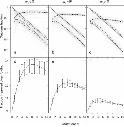
wild-type proteins chosen to be near the average stability of folded mutants (Fig. 1.3b,e)— the case ideally modeled by a mean-field treatment—the agreement is excellent. As expected, the model over-predicts the fraction folded for lower-than-average-stability wild-type sequences, and under-predicts in the opposite case, in both cases biasing the fraction of improved mutants in the same direction. The full model of Bloom et al. properly accounts for initial stability differences11,14. The main contribution of this work, Eq. 1.3, proves a reasonable approximation for the probability of improvement in a folded sequence (Fig. 1.3c-e).

These results justify the formulation of Eq. 1.1, in the sense that the problem of improvement, at least in this case, can be usefully subdivided into the problem of folding and the problem of improvement given folding. They also suggest that the model can indeed explain the gross average behavior of key terms in Eq. 1.1, although for larger improvement targets, the model deviates more significantly, because more mutations are required to obtain any improvement at all (not shown). However, the mathematical model’s reasonable performance does not offer any insight into whether the underlying intuitions used to construct it are correct.

Accordingly, I examined the predictions regarding the fitness mean and variance made above using a simple correlation analysis. Table 1.1 reports squared Spearman rank correlations (r2) of the mean and variance of folded-mutant fitness (hereafter, folded fitness) with the fraction of improved variants among folded mutants, quantifying the fraction of the latter’s variation explained by each statistic. All predictions were confirmed. In addition, as expected, the mean folded fitness gravitated upward with mutational distance for w₀ <w (Spearman r = +0.50, P << 10−9), hovered virtually unchanged for

w

w₀ ≈ (r = +0.09, not significant), and declined sharply for w₀ >w (r = −0.95, P << 10−9). These findings suggest the intuitive treatment above has some validity.

“Under what conditions should I increase the mutation level of my library?” Considering only folded sequences, the answer is, “Almost always,” while considering folded and unfolded sequences—the actual problem one faces at the bench—the answer is, “Almost never.” Past the first mutation or two, diversity-driven gains in improvement are more than offset by diversity-driven losses in folded proteins.

The dominance of misfolding depends in large part on ν, raising the question of how the neutralities of these lattice proteins compare to those of real proteins. While neutralities have been measured for few proteins, Bloom et al. report estimates ranging from 0.38 to 0.55 for proteins of diverse structures, and in Chapter 2, I derive a neutrality of 0.54 from experimental mutagenesis data for the β-lactamase PSE-4. The lattice proteins assayed here have neutralities around 0.6, comparable to real proteins. (It is surprising and fortunate that these compact lattice proteins have similar thermodynamic stabilities [5–10 kcal/mol] and neutralities to real proteins. As we will see in Chapter 6, these biophysical properties are crucial to understanding tradeoffs in the natural evolution of proteins.)

These results bear on the question of optimal diversity in protein engineering. I observe that, consistent with previous results28,29, there can be such a thing as too much diversity even when folding is preserved. However, excess diversity is practically irrelevant in these simulations, because by the time such effects kick in, half the protein has been mutated and virtually all mutants are misfolded. Instead, the dominant tradeoff is between folding and diversity4. Optimal diversity balances the need to explore with the need to survive.

roughly additive. However, they also demonstrate that folding concerns should not be absent.

But what if mutations—particularly the ones which confer improvement—are simply not additive21? This question is also taken up in Chapter 2, where my aim is to explain the puzzling observation that high-error-rate random mutagenesis using a popular protocol produces improved proteins more often than low-error-rate mutagenesis, a finding claimed to suggest mutational coupling or non-independence. I find little evidence for this claim. (However, it should be noted that if a protein’s function has been optimized by point mutation, but is still improvable, the mutations which confer improvement must logically be coupled in the strong sense of being individually deleterious, but cooperatively beneficial.)

If Chapter 2 describes a case of seeing mutational coupling where none exists, Chapter 3 is a case of finding strong coupling where it had not been fully appreciated or even noted, in the first comparison of the efficiency of protein recombination versus mutation in exploring the space of functional (read: folded) sequences.

Methods

Lattice protein folding

Lattice proteins were folded as described30; those methods are paraphrased here for convenience. The energy of a conformation i is

∑

i A A

E γ( , )

where γ(A_j,A_k) is the contact energy between amino acids Aj at position j and Ak at position k in the sequence, and Δi_jk is 1 if the two amino acids are in contact in conformation i and zero otherwise. The partition function is =

∑

i

T k E_{i B}

e

Z / where i runs

over all 1,081 conformations and k_BT =0.6 kcal/mol is the Boltzmann constant times the effective temperature T. The free energy of folding is defined as

] ln[ E /k T

B f

f E k T Z e f B

G = + − −

Δ

where E_f is the energy of the sequence in its the lowest-energy conformation. Stability, the free energy of unfolding, was then ΔG=−ΔG_f .

Accelerating interrogation of lattice protein folding

levels, where most proteins are highly destabilized, and sped up the overall experiment by roughly an order of magnitude.

Mutagenesis

To generate the results analyzed in this chapter, I began by finding a protein with a target structure and a minimum stability. I chose structure 574 because it is highly designable (more sequences fold to it as their native conformation than any other sequence, my unpublished observation) and is therefore intrinsically mutationally tolerant, allowing access to very high mutation levels with some tractable probability of finding folded sequences. Test runs revealed that, under the conditions I studied (minimum ΔG = 4 kcal/mol for folded sequences), the stability of folded mutants converged around 4.6 kcal/mol, providing an estimate of the average fitness of folded mutants. I then chose three stability ranges for wild-type sequences: ΔG = 4 to 4.6 kcal/mol (below-average fitness), ΔG = 4.6 to 4.65 kcal/mol (average fitness), and ΔG = 5.3 to 5.6 kcal/mol (above-average fitness). Sequences adopting the target conformation with stabilities in these ranges were found by random sequence generation and adaptive walks. Wild-type sequences were obtained by evolving initial sequences for 10,000 generations at a low mutation rate and stability constrained to the ranges given above.

Once a wild-type sequence was found, it was subjected to point mutations as described in the text. Folding (stability greater than or equal to 4 kcal/mol) was assessed for all mutants, and exact stability (hence fitness) was assessed for folded proteins.

Statistical analyis

Table 1.1: Correlation analysis of folded-mutant fitness properties on the likelihood of improved function.

Fraction of B’s variance explained by A (Spearman r2)* Relationship (A & B) w₀ <w w₀ ≈w w₀ >w

Var[folded fitness] & Pr(improved)

0.39 0.73 0.51

Mean+Var[folded fitness] &

Pr(improved) 0.41 0.91 0.35

Mean[folded fitness] & Pr(improved)

0.38 0.84 0.22

C h a p t e r 2

COUPLING IN HIGH-ERROR-RATE RANDOM MUTAGENESIS1

I don’t recall your name but you sure were a sucker for a high inside curve.

Bill Dickey

Summary

The fraction of proteins which retain wildtype function after mutation has long been observed to decline exponentially as the average number of mutations per gene increases. Recently, several groups have used error-prone polymerase chain reactions (PCR) to generate libraries with 15 to 30 mutations per gene on average, and have reported that orders of magnitude more proteins retain function than would be expected from the low-mutation-rate trend. Proteins with improved or novel function were disproportionately isolated from these high-error-rate libraries, leading to claims that high mutation rates unlock regions of sequence space that are enriched in positively coupled mutations. Here, we show experimentally that error-prone PCR produces a broader non-Poisson distribution of mutations consistent with a detailed model of PCR. As error rates increase, this distribution leads directly to the observed excesses in functional clones. We then show that while very low mutation rates result in many functional sequences, only a small number are unique. By contrast, very high mutation rates produce mostly unique sequences, but few retain fold or function. Thus, an optimal mutation rate exists which balances uniqueness

1 _{Adapted from Journal of Molecular Biology 350, D. Allan Drummond, Brent L. Iverson, George Georgiou, and Frances}

Introduction

Laboratory evolution has been used to improve protein properties by mimicking natural evolution’s stepwise exploration of sequence space7, steadily improving protein activity or thermostability through repeated rounds of low-frequency mutation and selection. Because the fraction of proteins retaining function declines exponentially with increasing numbers of amino acid substitutions11,15-17 (cf. Chapter 1), low mutation rates seek to create mutational diversity without destroying activity26 so that improved clones can be found. Recently, several groups reported construction of mutant libraries using high-mutation-rate error-prone polymerase chain reactions (EP-PCR) to probe distant regions of sequence space for an antibody fragment (up to an average m_nt = 22.5 nucleotide mutations per gene)16,32, hen egg lysozyme (up to mnt = 15.25)33, and TEM-1 β-lactamase (up to

nt

m = 27.2) 21. Where both high and low error rates were assessed, the exponential trend in loss of function established for low m_nt was spectacularly violated at the highest rates, with orders of magnitude more functional clones isolated than would be expected16,32,33. Two studies reported improved or novel function more often in these high-mutation-rate libraries16,21, leading to suggestions that low mutational pressure may not be optimal16,21 and that hypermutagenesis can, without an exponentially increasing cost in inactivated sequences, explore multiple interacting mutations inaccessible to low-error-rate mutagenesis21. These putative interactions could involve synergistic interactions to increase function directly, or combinations in which one or a few mutations increase function at the cost of folding or structural stability, the negative effects of which are suppressed by additional compensatory stabilizing mutations elsewhere in the protein.

“Why is there sex?”36 Moreover, the discovery of reservoirs of positively interacting mutations would fundamentally change strategies for in vitro enzyme engineering by evolutionary methods21. Therefore, a careful analysis of these results is imperative.

Quantitative analysis of high-frequency mutagenesis results often assumes a Poisson distribution of mutations in error-prone PCR, an idea introduced by Shafikhani et al.17. This group’s careful study on B. lentus subtilisin found an accurately reproducible exponential decline in fraction functional in all libraries where functional proteins were found, up to m_nt =15, contrary to the upward trend reported later.

To examine the mutational distribution generated by high-error-rate error-prone PCR, we constructed two large libraries of single chain Fv (scFv) antibody mutants. The wildtype scFv antibody fragment derived from the 26-10 monoclonal antibody37 binds digoxigenin with high affinity, and has been expressed as a fusion to the E. coli outer membrane protein Lpp-OmpA’, allowing detection of mutants binding fluorescent-dye-conjugated digoxigenin by fluorescence-activated cell sorting (FACS)16. Libraries were assayed for mutant retention of wildtype affinity for digoxigenin (briefly, retention of function). These libraries were constructed and assayed exactly as in a previous study16, making the results of both studies directly comparable. We were able to determine how the mutational statistics relate to PCR experimental parameters and to retention of function.

for a discussion of why, in most cases, loss of folding is the likely culprit for loss of function.

Results

Distribution of mutations generated by error-prone PCR

The probability Pr(f) that an error-prone PCR-amplified sequence retains function can be obtained as follows (here, and in all that follows, we elide the conditioning on the initial sequence introduced in Chapter 1). Sun38 modeled error-prone PCR by assuming n thermal cycles during which DNA strands are duplicated with probability λ, the PCR efficiency (assumed constant, realistic for large amounts of starting template39,40), resulting in d=nλ DNA doublings and an average of mnt nucleotide mutations per sequence. The

mutational distribution under these assumptions can be written38, with

λ λ n m

x= nt (1+ ), as

( )

_∑

= λ λ , (2.1)

which has mean m_nt and variance _⎟⎟

⎠ ⎞ ⎜⎜ ⎝ ⎛ + = + = d m m n m m m nt nt 2 nt nt 2 ₁ nt λ

σ . At large

nt

m , small n or low λ, all of which broaden the variance, deviation from the Poisson assumption that the variance is equal to the mean m_nt can be profound. We call Equation 2.1 the PCR distribution.

Results of mutagenesis

Both libraries were assayed for retention of wildtype-like binding to digoxigenin (retention of function) and 45+ naïve clones from each library were sequenced.

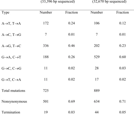
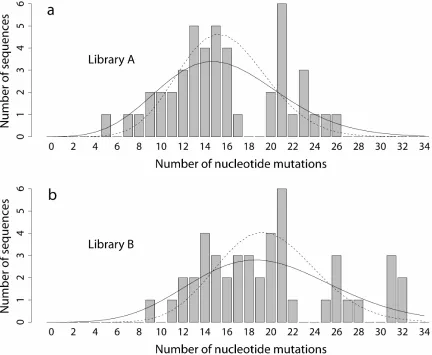
Poisson-distributed mutations will have equal mean and variance, while PCR-distributed mutations will always have a variance larger than the mean. Figure 2.1 shows the distribution of nucleotide mutations observed in library A (46 sequences) and library B (45 sequences); summary statistics are shown in Table 2.1, and mutational spectra are reported in Table 2.2.

While visual inspection of the mutation histograms overlayed with the theoretical distributions cannot distinguish between the two models, the relevant statistics are stark and favor the PCR distribution while rejecting the Poisson distribution. For library A, m_nt = 15.8 and σ_m2_nt= 26.3; for library B, m_nt = 19.8 and σ_m2_nt= 36.1 (Table 2.1). The probability of measuring variances at least this large given an underlying Poisson distribution with the observed mean is P < 0.005 for library A and P < 0.001 for library B; the joint probability of observing two libraries with variances this high is P < 10−5. With a PCR efficiency of λ = 0.6 (18 doublings), the PCR distribution yields expected variances of 29.6 (library A) and 41.4 (library B), consistent with the observed values.

Using a likelihood ratio test on the mutational samples (see Methods), we reject the Poisson distribution in favor of the PCR distribution with two additional degrees of freedom (n and λ) for library A (χ2 = 7.39, P < 0.025) and for library B (χ2 = 8.63, P < 0.025). (Using two additional degrees of freedom is conservative, since n is fixed in each experiment.) Thus, the PCR distribution (Eq. 2.1) better describes the data than the previously assumed Poisson model.

Retention of protein function after mutation

aa )

Pr(f m_aa =νm , where the neutrality ν can be interpreted as the average fraction of functional one-mutant neighbors on the protein-sequence-space network34,41 (cf. Chapter 1). This assumption is consistent with experimental results obtained without using PCR15 and with theoretical considerations11. This model assumes no average epistasis.

The probability a nucleotide mutation produces a nonsynonymous change is assumed to be binomial with parameter p_ns, corresponding to the assumption that mutations hit distinct codons. This assumption and the value p_ns= 0.7 appear realistic16 (the precise parameter value will vary somewhat based on a gene’s codon composition). In the following analysis, nonsynonymous changes include insertions, deletions, mutations to stop codons, and mutations that change the encoded amino acid: p_ns = p_ins + p_del + p_stop + p_aa. The first three types of changes are assumed to truncate and inactivate the encoded protein; we assume they constitute a fraction p_tr = p_ins+ p_del+ p_stop ≈ 0.05–0.07 of mutations (e.g., see ref. 19, supporting information) and use the value p_tr = 0.06 for our calculations. The probability that a nonsynonymous mutation does not truncate the encoded protein (i.e. only changes the encoded amino acid) is (1− p_tr /p_ns). The probability a sequence with m_nt nucleotide mutations retains function includes all these effects and is therefore

. ) )) / 1 ( 1 ( 1 ( ) / 1 ( ) 1 ( changes) acid amino | Pr ) | non trunc. Pr( ) | Pr( Pr nt ns ns ns nt ns nt ns nt ns ns ns tr ns tr ns ns 0 _ns nt

0 ns nt ns ns

nt m m m m m m m m m m p p p p p p p m m m (f m m m ) m (f − − − = × − × − ⎟ ⎟ ⎠ ⎞ ⎜ ⎜ ⎝ ⎛ = = − = =

∑

∑

ν (2.2)

Under the assumption of Poisson-distributed mutations, Shafikhani et al.17 showed that, if a fraction qi of nucleotide mutations inactivate a protein, the fraction functional declines

exponentially as _e−mnt qi. Because

ns ns tr/ )) 1

(

1 p p p

(

ns ns tr nt 1 (1 / ))

)

Pr(f =e−m ( −ν −p p p in a Poisson-distributed library. This exponential decline

became the experimental expectation for subsequent groups, leading to surprise when functional mutants were later found in great excess at high average mutation rates. By combining Equations 2.1 and 2.2 and assuming gene length L→∞—a mild assumption

when m_nt <<L—we find the probability a sequence from the library will retain function is n m p p p n m e m m f f

∑

= − − + − ⎟⎟ ⎟ ⎟ ⎠ ⎞ ⎜⎜ ⎜ ⎜ ⎝ ⎛ + + = = 0 )) / 1 ( 1 ( ) 1 ( nt nt nt ns ns tr nt 1 1 ) Pr( ) Pr( ) Pr( λ

λ λ ν

λ

. (2.3)

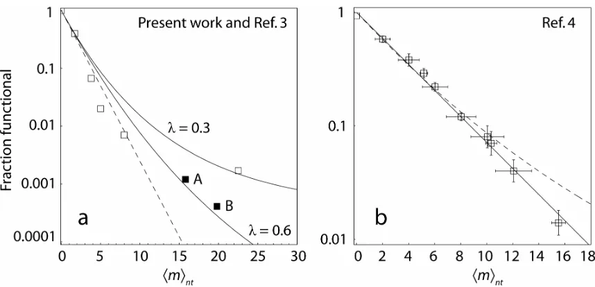
Equation 2.3 makes several predictions. In the limit of many thermal cycles n, all else equal, the original expectation _Pr(f)=_e−mnt (1−ν(1−ptr/pns))pns _{(above) is recovered. If the} number of thermal cycles n is proportional to m_nt , following the protocol of Shafikhani et al., then Pr(f) should be a perfect exponential in m_nt , which is precisely what this group reports. However, if n is fixed as in other studies16,21,33, then Pr(f) curves upward relative to an exponential decline as m_nt increases. PCR efficiency λ decreases with increasing m_nt 42, which increases the expected curvature. In other words, there will be more functional sequences than predicted by the exponential decline.

Using the previously reported scFv antibody data16 for low m_nt , where the Poisson assumption is not unreasonable, and the reported value q_i =0.6, we can estimate ν ≈0.2 for the antibody binding task. For the subtilisin data17, we similarly use the reported

27 . 0 =

i

2.2b). The agreement is quite good and demonstrates that the excess of functional clones can in fact be consistent with an underlying exponential relationship between number of amino acid substitutions and probability of retained wild-type function. To further test our analytical predictions, we simulated single-round error-prone PCR using template DNA strands encoding a folded “wildtype” lattice protein. The amplified DNA was translated into lattice proteins which were scored as functional if they retained the fold and thermostability of the wildtype. We observed excellent agreement with Equation 2.3 (see Supplemental Material for this chapter).

The reason for deviation from an exponential decline is hinted at in the limit of large average mutation rates, when the exponential part of Equation 2.3 vanishes and Pr(f) approaches a constant, Pr(f)→(1+λ)−n. For a mutationally fragile protein such as the scFv antibody performing the digoxigenin binding task, this can occur at experimentally accessible mutation rates, as can be seen most clearly in the library originally reported16 and revisited by Georgiou32. As the mutation rate increases, the antibody fragment becomes “quite insensitive to mutational load” and Pr(f) flattens out at a value of roughly 0.0018 32. Most interestingly, this limiting value is a function only of the PCR conditions, and does not depend on the protein at all.

Why are improved mutants found more often in high-error-rate libraries?

If statistical effects of the mutagenesis protocol can explain the dramatic deviation from exponential in the fraction of functional sequences without recourse to epistasis, why are high- m_nt libraries enriched in improved clones, despite a smaller number of clones retaining any function? To address this question, we now explore another consequence of PCR’s broad mutational distribution.

The effective size of a library is not the number of mutants screened, the number usually reported, but rather the number of unique mutants screened. In a library of 106 transformants of the scFv antibody gene (726 bp, 242 aa) with an average of one mutation per sequence, most of the 2,178 possible 1-mutants will occur on the order of 100 times, reducing the effective library size by roughly two orders of magnitude. Most mutagenesis is concerned with protein sequences, where additional losses occur. Truncations due to frameshift mutations or mutations to stop codons eliminate a significant fraction of sequences. With one nucleotide mutation per codon, an average of 5.7 amino acid substitutions (out of a maximum of 19) are accessible due to the conservatism of the genetic code, for a total of 242 × 5.7 = 1,379 accessible amino acid sequences with one substitution. (We ignore the effects of synonymous mutations.) One million transformants thus yield just over one thousand unique protein sequences, about a 1,000-fold reduction in the effective library size.

We estimate the number of unique sequences in an error-prone PCR library in the following way. We derive the distribution of nonsynonymous substitutions Pr(m_ns) after error-prone PCR, estimate the number of non-truncated amino acid sequences N_mnswith each m_ns in a library of a given size, compute the expected number of unique sequences U_mns at each

ns

m by accounting for recurrence among the ns m

With PCR conditions denoted as before and an average number of nucleotide mutations per sequence m_nt , what is the distribution of the number of nonsynonymous substitutions per sequence Pr(m_ns)? We assume, as before, that each nucleotide mutation causes a nonsynonymous change with probability p_ns, so we obtain

( )

( )

( )

∑

∑

y= nt ns(1+ ). That is, the distribution of nonsynonymous substitutions )

Pr(m_ns is equivalent, in form, to the distribution of nucleotide mutations Pr(m_nt), but with an average of m_ns = m_nt p_ns substitutions. For simplicity, we will drop the subscript for nonsynonymous substitutions and use m.

Of the sequences with m nonsynonymous substitutions, some will also be truncated by frameshifts or stop codons. Because we treat all truncations as nonsynonymous changes, the fraction of non-truncated sequences with m substutions is Pr(non-truncated|m) =(1−p_tr /p_ns)m. Given an error-prone PCR library of N transformants, N_m= N Pr(m) Pr(non-truncated|m) on average are non-truncated proteins with m amino acid substitutions.

Of these proteins with m substitutions, how many unique sequences exist? Only one unique sequence has m = 0. For any m there are on average _m m

m L M /3_⎟⎟5.7

⎠ ⎞ ⎜ ⎜ ⎝ ⎛

= total unique

Given N_m samples, how many of these M_m unique proteins can we expect to find? This is the classic “coupon collector problem”43 and directly addresses the question of mutant recurrence, since any sample either yields a new, unique protein or one that has been sampled before. The expected number of unique sequences produced by equiprobably sampling M_m sequences N_m times is

). 1 ( ) / 1 1

( m Nm/Mm

m N

m m

m

m M M M M e

U = − − ≈ − − (2.5)

For example, to sample 99% of the M_m= 1,379 accessible 1-mutants of scFv requires 4.6-fold oversampling (N_m= 6,350 samples) on average. Taking 1,379 samples, N_m=M_m, on average yields only 872 unique proteins, or 63% of the total. In practice, for proteins of a few hundred amino acids and libraries of a few million transformants, recurrence need only be considered for small values of m (m < 3), because sequence space becomes large enough to make recurrence extremely unlikely at higher m values so that U_m≈N_m. The total number of unique sequences in a library is simply the sum over all unique sequences with a specific number of substitutions:

∑

=

= /3 0

L m m

U

U . (2.6)

Of greater interest is the expected number of unique sequences in the library that are expected to retain at least wildtype function, because these sequences are a superset of potentially improved sequences. We can estimate the number of unique, functional sequences as

∑

=

= /3 0

L m

m m f U

U ν . (2.7)

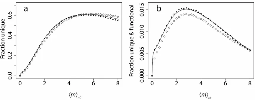
Figure 2.3b shows the fraction of unique, functional sequences Uf/N obtained from the

same simulations as in Fig. 2.3a, with Eq. 2.7 plotted for comparison. Biases in mutation frequencies decrease the fraction of unique sequences, but preserve the overall form. Results using unbiased frequencies are predicted accurately by our theoretical treatment. Clearly, low-error-rate libraries suffer from dramatic mutant recurrence, an effect avoided at high error rates. Improved proteins are found often in high-error-rate libraries because these libraries contain more unique functional sequences.

Optimal random mutagenesis

A typical and important goal in protein engineering is to improve an existing protein function, for example by increasing catalytic rate, thermostability, binding affinity, or specificity. While rational engineering has made significant strides, high-throughput screening of large mutant libraries for improved clones is both a dominant strategy to achieve this goal and an area of active research32.

The optimum depends on the number of transformants sampled, the PCR protocol used, and the wildtype protein being mutated, among other parameters. Figure 2.4a compares predicted optimal mutation rates under identical PCR conditions for the scFv antibody (ν ≈0.2), depending on whether a thousand or a million clones are screened. The difference, 1.3 average nucleotide substitutions, corresponds to one amino acid substitution on average. Figure 2.4b compares predicted optimal mutation rates under identical conditions and with the same wildtype protein, but using 30 thermal cycles (as in the present work) in one case and 2 cycles (as in ref. 21) in the other. A difference of one nucleotide mutation results. Optimal rates also depend on protein mutational tolerance as reflected by ν : the more tolerant the protein, the higher the optimal mutation rate (not shown).

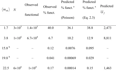
Table 2.3 lists estimates for U_f given the scFv library experimental conditions reported here and previously16. Despite the over 200-fold lower observed percentage of functional transformants isolated from the highest- m_nt library relative to the lowest, and the 14-fold fewer functional sequences observed, only 60% fewer unique functional sequences are expected in the highest- m_nt library. Given the experimental parameters of the

highest-nt

m library and altering only the mutation rate, the rate m_nt = 11.0 is predicted to produce more unique functional sequences (>10,000) than any of the reported libraries. The optimal mutation rate given the highest- m_nt experimental parameters is predicted to be roughly m_nt = 3.0, which is predicted to yield >34,000 unique, functional sequences. These results do not account for gains in probability of improvement treated in Chapter 1, but such gains are expected to be small relative to the cost of loss of folding and function. Discussion

of functional and, for at least some enzymatic tasks, improved proteins has been advanced several times, with significant experimental evidence to bolster the claims. We have shown that a more accurate model of error-prone PCR than previously used, due to Sun38, is required to adequately describe the mutational distribution resulting from high-error-rate error-prone PCR. This model, in turn, provides straightforward explanations for the previously observed experimental findings: 1) the excess functional proteins observed at high m_nt is predictable using our Equation 2.3, is due to low-mutation sequences generated early in the reaction, and is consistent with an exponential decrease in retention of function with amino acid substitution level; and 2) loss of functional sequences at high mutation rates can be balanced by diversity in the form of more unique sequences, improving sampling of sequence space and leading to a higher probability that improved mutants will be found if they exist. We have demonstrated the often-overlooked importance of accounting for recurrence of mutants when estimating how much of sequence space a library covers, extending previous work on modeling effects of mutational bias44. With our simple definition of library optimality as maximizing the number of unique, functional proteins, these two observations lead to an optimal mutation rate for error-prone PCR which can be estimated using our analytical results. However, optimal mutation rates are both protocol- and protein-dependent. Optimal rates derived for error-prone PCR using one set of conditions do not necessarily hold for another set (Fig. 2.4), and are highly unlikely to hold for saturation mutagenesis or site-directed mutagenesis, for which uniqueness is rarely a problem and the distribution of mutation levels in a typical library is tight and easily controllable.

due to the conservative nature of the genetic code. While ν relates simply to the “structural plasticity” q_i =(1−ν(1− p_tr /p_ns))p_ns proposed by Shafikhani et al. 17, our results show that the emergence of a perfect exponential decline in their experiments likely depended both on a fundamental property of proteins and the particular experimental protocol employed. We also distinguish between genetic mutations which produce truncated protein products, essentially all of which lack function, and those which produce full-length proteins whose structural properties determine whether mutations are tolerated. We believe ν more accurately captures the idea of structural plasticity.

Because optimal mutation rates depend on ν , we can suggest measures which influence ν and which therefore may be used to manipulate the optimal mutation rate. All else being equal, proteins with higher thermodynamic stability (free energy of unfolding) have a higher ν 11 and tolerate more destabilizing substitutions, suggesting that more stable variants of a protein represent more promising departure points for mutagenesis. If longer proteins are more tolerant of substitutions, as seems plausible, then longer genes will tend to have higher optimal mutation rates. Codon usage may influence ν indirectly, through protein expression; in cases where high protein expression is required for the relevant function, replacement of rare codons with common synonyms may allow higher mutation rates. When a protein’s crystal structure is available, ν can be estimated computationally11. We also note that the exponential decline in fraction functional holds when many mutations are introduced, as in the present work, but may not always hold for small numbers of mutations11 (e.g., see Fig. 1.3 in the previous chapter).

protein, hindering its folding or exposing it to proteolysis or irreversible misfolding without actually destroying the function of the natively folded molecule. The dominant effect of most random mutagenesis is changes in the primary sequence of a target protein, most of which disrupt native function, and our simple treatment appears to work well under these circumstances.

Our results also illuminate potentially serious methodological flaws in previous studies. For example, the accuracy in measuring average library mutation rate by nucleotide sequencing depends on the variance of the mutational distribution, which at high mutation rates is far broader than that of the Poisson distribution previously assumed. The expected standard error of measurement on a library with m_nt average mutations assessed by sequencing N_seq clones is σ_m/ N_seq = m_nt

(

)

mutations per coding region of a 1,088 base-pair gene constructed using 2, 5, 10 and 20 thermal cycles with m_nt measured by sequencing at least 2,500 base pairs, effectively

seq

N = 2.5. Even if the true value of m_nt is as measured and perfect PCR efficiency assumed, these measurements have an expected 1σ standard error of 4.3, 6.5, 5.4 and 5.3 mutations per gene, respectively, calling into question the actual levels of hypermutagenesis achieved in these experiments.

The analysis presented here has important consequences for understanding the natural and directed evolution of proteins. Importantly, we have provided a thorough analysis of an apparent manifestation of mutational epistasis.