Wall Follower Autonomous Robot Development Applying Fuzzy Incremental Controller

(1)

Wall Follower Autonomous Robot Development Applying

Fuzzy Incremental Controller

Dirman Hanafi, Yousef Moh Abueejela, Mohamad Fauzi Zakaria

Department of Mechatronic and Robotic Engineering, Faculty of Electrical and Electronic Engineering, Universiti Tun Hussein Onn Malaysia, Parit Raja, Malaysia

Email: dr_dirman@yahoo.com

Received September 18, 2012; revised October 18, 2012; accepted October 25, 2012

ABSTRACT

This paper presents the design of an autonomous robot as a basic development of an intelligent wheeled mobile robot for air duct or corridor cleaning. The robot navigation is based on wall following algorithm. The robot is controlled using fuzzy incremental controller (FIC) and embedded in PIC18F4550 microcontroller. FIC guides the robot to move along a wall in a desired direction by maintaining a constant distance to the wall. Two ultrasonic sensors are installed in the left side of the robot to sense the wall distance. The signals from these sensors are fed to FIC that then used to de- termine the speed control of two DC motors. The robot movement is obtained through differentiating the speed of these two motors. The experimental results show that FIC is successfully controlling the robot to follow the wall as a guid- ance line and has good performance compare with PID controller.

Keywords: Autonomous Robot; Wall Follower; Fuzzy Incremental Controller; Embedded System

1. Introduction

Wheeled robots are mechanical devices capable of mov- ing in an environment with a certain degree of autonomy. Autonomous navigation is associated to the availability of external sensors that get information of the environment through visual images or distance or proximity measurements. The most common sensors are distance sensors (ultrasonic, laser, infrared, etc) able to detect obsta- cles and measure the distance to walls close to the robot path. When advanced autonomous robots navigate within indoor environments (industrial or civil buildings), they have to be endowed the ability to move through corridors, to follow walls, to turn corners and to enter open areas of the rooms [1-4]. The degree of a mobile robot ability to move around autonomously in its environment deter- mines its best possible application such as tasks that in- volve transportation, exploration, surveillance, inspection, etc.

In attempts to formulate approaches that can handle real world uncertainty, researches are frequently faced with the necessity of considering tradeoffs between de- veloping complex cognitive systems that are difficult to control. Furthermore, they adopt a host of assumptions that lead to simplified models which are not sufficiently representative of the system or the real world. The latter option is a popular one which often enables the formula- tion of viable control laws. However, these control laws are typically valid only for systems that comply with im-

posed assumptions, and furthermore, only in neighbor- hoods of some nominal state. Recent research and application employing non-analytical methods of computing such as fuzzy logic, evolutionary computation, and neu- ral networks have demonstrated the utility and potential of these paradigms for intelligent control of complex systems. In particular, fuzzy logic has proven to be a convenient tool for handling real world uncertainty and knowledge representation [3,5-7]. When a mobile robot is designed, the three key questions that need to be an- swered by the robot are: (WhereamI, WhereamIgoing, and howdoIgetthere).

So that, to reach these three answers the robot has to have a model of the environment. After that it needs to perceive and analyze the environment to find its position within the environment. The plan and execution of the movement will then be finally defined by its control method. Most of the current practical robot technology in industries is focused on areas such as positioning, teach- ing-playback, and two-dimensional vision [8].

The first section of this paper gives introduction about mobile robot development. The second section explains related work with this paper. The third section gives in- sight into the methodology to develop a wall follower mobile robot.

2. Related Work

(2)

robotics motion control development. It is a heavily re- searched area due to both the challenging theoretical na- ture of the problem and its practical importance. Previous work in autonomous mobile robot control generally involves line following, wall following, path tracking control, and so on.

In order to follow a wall and navigate, image process- ing techniques can be used to detect perspective lines to guide the robot along the centre axis of the corridor. This technique requires cameras that can be expensive. Previ- ous work in autonomous mobile robot control generally involves path planning and path tracking control. It can be classified into the following four categories: linear [9,10], nonlinear [11,12], geometrical [13], and intelligent [3,13] approaches. Using two switches on the left of the robot to follow left wall and a bumper switch to detect an obstruction in front is suggested in [6,7]. A genetic algorithm using Fuzzy Logic Controller is developed in [14]. A multivariable control and ultrasonic range finders for the measurement of a distance are being used for wall tracking robot in [15]. A Fuzzy Logic Controller is used to drive a robot parallel to the wall with the help of ultrasonic sensors in [16]. In this paper fuzzy incremental controller (FIC) is applied to improve the performance of wall follower robot with input from ultrasonic sensors.

3. Methodology

3.1. Robot Movement Principle

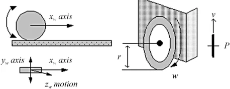
The autonomous robot is modeled as a rigid body that satisfies a nonholonomic constraint, which means the motion of the system is not completely free. They are in which the instantaneous velocities of system components are restricted, thereby limiting the local movement of the system. This means that the mobile robot cannot move sideways and based on the principle of a rolling wheel.

Figure 1 shows an idealized rolling wheel [17]. The wheel is free to rotate about its axis (Yw axis). The robot

exhibits preferential rolling motion in one direction (Xw

axis) and a certain amount of lateral slip. For lower velocities, rolling motion is dominant and slipping can be neglected.

Where, r = wheel radius, V = wheel linear velocity and

Figure 1. An idealized rolling wheel.

ω = wheel angular velocity.

In this case, some assumptions as below are used.

 No slip occurs in the orthogonal direction of rolling (non-slipping).

 No translation slip occurs between the wheel and the floor (pure rolling).

 At most one steering link per wheel with the steering axis perpendicular to the floor.

3.2. Robot Model

Deriving a model for the whole robot’s motion is a bot- tom-up process. Each individual wheel contributes to the robot’s motion and, at the same time, imposes constraints on robot motion. Wheels are tied together based on robot chassis geometry, and therefore their constraints combine to form constraints on the overall motion of the robot chassis. Other case the forces and each wheel constraints must be expressed with respect to a clear and consistent reference frame. The develop robot is a two-wheeled mobile robot (Differential Drive) whose position is defined by three Coordinates (3 DOF) in a plane



x y, ,



.

Figure 2 below shows a two-wheeled robot, where P is the motion center of the autonomous robot and the grav- ity centre of the platform. Where,



x,y



represents li-

near speed or tangential velocity and  is the angular velocity.

Kinematics is the study of the mathematics of motion without considering the forces that affect the motion. It deals with the geometric relationships that govern the system. It develops a relationship between control parameters and the behavior of a system in space. The model of the robot is as shown in Figure 3. The linear speed of the right and the left wheel are related to the angular speed as follows:



Right,Left



y

vy vx

 _

[image:2.595.59.288.628.717.2]

x

Figure 2. The model of the mobile robot.



d R

left v



right v

R v

Figure 3. Robot parameters.

(3)

Right r Right

  

Left r Left

(1)

   (2) where, r is the radius of the wheel. Right and Left is

angular velocity of the right and left wheels respectively.

R

 and R are the velocity and angular velocity of the

robot respectively.

[image:3.595.316.538.85.198.2]

The total linear and angular speed of the robot can be calculated as Equations (3) and (4). In order to specify the position of the robot on the plane, a relationship between the global reference frame of the plane and the local reference frame of the robot are established as in

Figure 3 [9,10]. The robot in a state of motion must al- ways rotate about a point that lies somewhere on the common axis of its two wheels. This point is often called the Instantaneous Centre of Curvature (ICC).

The robot’s coordinates

 

x y,

 

 changed with respect to time can be calculated us- and its orientation ing the following equations.



Right Left



2

 

R

  (3)



Right Left



t   d

d d

R

    (4)

d dx t x _Rcos (5)

dy td  y _Rsin (6)

R

 

 

0 0

(7)

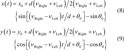
Integrating Equations (5) and (6), and taking the initial positions to be x x and y

 

0 y₀with initial orientation 0 yields:

 



 









Right Leftft Right0 Left0



2

sin t d sin

 

0 Right

x d  Le

x t           

 



 



   (8)







0 Right Left Right0 Left0



2

cos

y t y d    

Right Left

cos   t d  

         cos 0 0 0 1 x R

  (9)

From the Equations (5)-(7), the kinematic model of the mobile robot with two independently driving wheels can be represented in Cartesian model as Equation (10).

sin

y

R

x  

y   _

                                          (10)

where, x and y are position variables,  is a heading direction angle (yaw angle), and



 ,







are the forward velocity and the rotational velocity (angular velocity) of the robot, respectively [12].





The position and the orientation of the autonomous robot are determined by a set of differential equations below: Right Left Right Left cos 0 2 sin 0 0 1 x y d   _ _         _{ } _ _   _ _{ } _    _{ } _ _           (11)

Equations (3) and (11) are extended to be:

Right

Left

1 2 cos 1 2 cos

1 2 sin 1 2 sin

0 1 x y d                  _       _{ } _          (12)

3.3. Wall Geometry and Robot Motion Model

In case of a different set of state is considered, it is possible to use the corridor navigation controller to enable the robot to follows a wall. This possibility is based on two tasks and very similar to each other. Where, the state are defined in relation to the wall as  and D.  is the angular deviation relative to the wall line and D is the distance of the robot from an imaginary line at a desired distance from the wall as represented in Figure 4 [10,18].

Two ultrasonic sensors are mounted in left side of robot and named as 1 and 2. Variable D is calculated

through the following equations:

S S

cos

D S  (13)



1 2



1 2

S  S S (14)

Using Pythagorean Theorem, relationship between  and sensors reading



S1S2



The develop controller is required to be back fed with the values of

is represented as Figure 5.

 and D at each instant. These values can be primarily obtained from ultrasonic measurements. For this case, the following Equations (15) and (16) can use to calculate the state variables.

[image:3.595.85.287.469.555.2]



D S L Sensor 1 Sensor 2

Figure 4. Wall geometry and sensors model.

L         2 1 S S

[image:3.595.347.500.498.623.2]

(4)









2



1 2 S S   2 1 2

cos S S L (15) Inference Mechanism









Defu zzi fi cati on Fuzzification 2 1 2

L2 S S

1 2

D S S (16)

Let consider that,  is very small and L is , the Equations (15) and (16) become:



S1S



2 2





1 2



1 2

D S S (17)



1 2



1 L S S

 





(18)

The angle error E_



, distance error d and total

error are evaluated based on the distance between the robot and the wall which represented by Equa- tions (19)-(21).

 

E





ETot



Re



Ed  f D (19)



1 2



E_  S S

Tot d

E E E

(20)



 

 

0

(21)

The right and the left angular velocity of each wheel are calculated using the following equation respect to the initial speed of each wheel  .



0 ETot



    



0 ETot



   Right 0 Left 0   (22) (23)

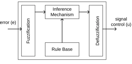
3.4. Fuzzy Logic Controller

Fuzzy logic is based on the principle of human expert decision making in problem solving mechanism. Where, the solution is described in a linguistic term or every spoken language, i.e., fast, slow, high, low, etc. [19,20]. In more complex cases, they include some hedge terms,

[image:4.595.309.539.83.195.2]

i.e., very high, not so low, etc. To represent such terms, a nonmathematical fuzzy set theory is needed.

Figure 6 shows the block diagram of fuzzy logic that consist four components: Fuzzification, Fuzzy rule based, Fuzzy inference and Defuzzification.

The design of fuzzy logic controller generally has the following step:

1) Design the membership function for fuzzification input and output variables.

2) Implement the fuzzy inference by a series of IF- THEN rules.

3) Inference engine derives a conclusion from the facts and rules contained in the knowledge base using various human expert techniques.

4) Process to maps a fuzzy set into a crisp set.

Fuzzy Incremental Controller (FIC) has main advan- tage that is smooth in signal control [21], therefore, it has been applied in this paper. Fuzzy Incremental Controller (FIC) as in Figure 7 has been developed to control wall follower robot. It has two input and two output variables.

error (e) _{control (u)}signal

Rule Base

Figure 6. Fuzzy logic block diagram.

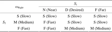
Input and output variables of FIC assumed have triangular membership function. Input variables are S1 and S2

(feedback sensor’s reading) and each of them have been assigned three linguistic values as Near (N), Desired (D) and Far (F). The controller output is used to control the change in angular velocity of the right and left wheel of the robot. The changes in angular velocities of the two wheels



_Right,_Left



have linguistic values: Slow (S), Medium (M) and Fast (F).

The membership functions graphs of FIC develop are shown in Figures 8-11. The triangular membership functions are used for their simplicity is quite commonly applied.

Generating the rules for fuzzy control system is often the most difficult step in the design process. It usually requires some expert knowledge of the plant dynamics. This knowledge could be in the form of an intuitive un- derstanding gained from experimenting, or it could come from a plant model which is then used in a computer si- mulation. Rule tabulation of each variable for wall follower robot is represented as in Tables 1 and 2.

4. Robot Construction

Figure 12 shows the physical construction of the wall follower robot developed respectively. It has two wheels on either side of its chassis. Each of these wheels has a separate DC motor. These motors run independently from each other with the help of PWM signals generated by the PIC18F4550 Microcontroller, and a driver IC SN 754410. Moreover, a caster wheel is used in to balance the entire chassis. The robot measures the distance from a wall on its left side. Two ultrasonic sensors are installed on the left side to aid in following a wall.

5. Controller Experimental Result

In this paper three kinds of controller have been applied for wall follower robot, they are fuzzy incremental controller (FIC), proportional differential (PD) controller and proportional integral and differential (PID) controller. Four graphs from each of controller responses are compared. First is Cartesian space, second is theta position of the robot, third is left back sensor response and finally is

(5)

[image:5.595.306.538.356.703.2]

Figure 7. FIC of wall follower robot block diagram.

Figure 10. Membership function of ωRight.

[image:5.595.56.288.467.676.2]

Figure 8. Memberships function of left back sensor (S1).

Figure 11. Membership function of ωLeft.

figures are in time unit (second). The experimental results are as Figures13-24:

Figure 9. Memberships function of right back sensor (S2).

Based on graphs above, FIC results give good performance, for angle of orientation, x position, y position Left front sensor response. The robot sets to follow the

(6)

[image:6.595.311.538.85.216.2]

Table 1. Rule tabulation of right wheel angular velocity.

S1 ωRight

N (Near) D (Desired) F (Far)

S (Slow) S (Slow) S (Slow) S (Slow)

M (Medium) F (Fast) S (Slow) S (Slow)

S2

F (Fast) F (Fast) M (Medium) M (Medium)

Table 2. Rule tabulation of left wheel angular velocity.

S1 ωLeft

N (Near) D (Desired) F (Far)

S (Slow) M (Medium) F (Fast) F (Fast)

M (Medium) S (Slow) F (Fast) M (Medium)

S2

[image:6.595.57.287.101.168.2]

F (Fast) S (Slow) S (Slow) S (Slow)

Figure 12. Robot physical construction.

Figure 13. (x, y) Cartesian space response under FIC.

[image:6.595.59.287.191.422.2]

Figure 14. Theta position of robot under FIC.

Figure 15. Left back sensor response of robot under FIC.

Figure 16. Left front sensor response of robot under FIC.

Figure 17. (x, y) Cartesian space response under PD.

Figure 18. Theta position of robot under PD.

 

x,

and y position as a whole. Besides that, FIC also produces lower overshoot for the motion and position of the robot in the orientation curve. Then the robot able to achieve reference position from the wall in short time

[image:6.595.309.538.243.383.2] [image:6.595.309.538.415.560.2] [image:6.595.56.290.432.721.2]

(7)

[image:7.595.58.289.82.207.2] [image:7.595.309.540.85.200.2]

Figure 19. Left back sensor response of robot under PD.

Figure 20. Left front sensor response of robot under PD.

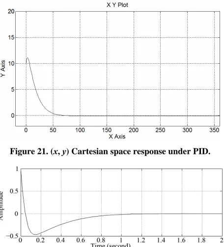
Figure 21. (x, y) Cartesian space response under PID.

Figure 22. Theta position of robot under PID.

compared with the other controllers.

The parameters response comparisons of each controller are listed in Table 3.

6. Conclusion

The wall following control of the autonomous robot has

[image:7.595.307.539.227.337.2]

Figure 23. Left back sensor response of robot under PID.

[image:7.595.58.290.234.347.2]

Figure 24. Left front sensor response of robot under PID.

Table 3. Controller response parameters comparison.

Fuzzy logic PD PID

Overshoot 0.24 0.29 0.46

Setting time 0.5 0.9 1

Error 1.2 × 10–13 _{6.5 × 10}–8 _{4.05 × 10}–5

been presented using ultrasonic sensors. The sensor data are used to measure and obtain the distance and orientation of the robot. Then, these data are utilized in the feedback controller. The FIC algorithm has been embedded in PIC18F4550 microcontroller for controlling the wall follower robot. The FIC responses good performance compared to PD and PID controller. The experimental results show the FIC controller gives lowest overshoot, shortest settling time and smallest error than PD and PID controller. It means FIC controller more suitable to be used in controlling wall follower robot.

7. Acknowledgements

This work has been supported by Faculty of Electrical and Electronic Engineering Universiti Tun Hussein Onn Malaysia.

REFERENCES

[1] R. Carelli, C. Soria, O. Nasisi and E. O. Freire, “Stable AVG Corridor Navigation with Fuse Vision-Based Con- trol Signals,” IEEE Proceeding of Industrial Electronics

[image:7.595.60.288.375.627.2] [image:7.595.307.538.383.443.2]

(8)

[2] R. Carelli and E. Freire, “Stable Corridor Navigation Controller for Sonar-Based Mobile Robots,” Technical Report, INAW, Universidad Nacional de San Juan, San Juan, 2001.

[3] R. Malhotra and A. Sarkar, “Development of a Fuzzy Logic Based Mobile Robot for Dynamic Obstacle Avoi- dance and Goal Acquisition in an Unstructured Envi- roment,” IEEE/ASME Proceeding of International Con-

ference on Advanced Intelligent Mechatronics, Kobe, 20- 24 July 2003, pp. 235-247.

[4] P. M. Peri, “Fuzzy Logic Controller for an Autonomous Mobile Robot,” Master Thesis, Cleveland State Univer- sity, Cleveland, 2005.

[5] D. Ratner and P. McKerrow, “Navigation an Outdoor Robot along Continuous Landmarks with Ultrasonic Sen- sing,” Robotics and Autonomous Systems, Vol. 45, No. 1, 2003, pp. 73-82. doi:10.1016/S0921-8890(03)00096-4

[6] R. Carelli and E. O. Freire, “Navigation Outdoor and Wall-Following Stable Control for Sonar-Based Mobile Robots,” Robotics and Autonomous Systems, Vol. 45, No. 3-4, 2003, pp. 235-247. doi:10.1016/j.robot.2003.09.005

[7] R. Benporad, M. Di Marco and A. Tesi, “Wall-Following Controller for Sonar-Based Mobile Robots,” Proceeding

of IEEE Conference on Decision and Control, San Diego, 10-12 December 1997, pp. 3063-3068.

[8] Japan Robot Society, “Summary Report on Technology Strategy for Creating a Robot Society in 21st Century,” 2001. http://www.jara.jp/e/dl/report 0105.pdf

[9] D. Simon, “Analyzing Control System Robustness,” IEEE Potentials, Vol. 21, No. 1, 2002, pp.16-19.

[10] B. Davies and W. E. R. Davies, “Practical Robotics: Prin- ciples and Applications,” Prentice Hall, Upper Saddle River, 1997.

[11] Z. Gao, “From Linear to Nonlinear Control Means: A Practical Progression,” ISA Transactions, Vol. 41, No. 2, 2002, pp. 177-189. doi:10.1016/S0019-0578(07)60077-9

[12] Z. Gao, Y. Huang and J. Han, “An Alternative Paradigm

for Control System Design,” Proceeding of IEEE Con-

ference on Decision and Control, Orlando, 4-7 December 2001, pp. 4578-4585.

[13] G. McComb and M. Preoko, “The Robot Builder’s Bo- nanza,” 3rd Edition, McGraw Hill, New York, 2006.

[14] R. Braunsting, J. Mujika and J. P. Uribe, “A Wall Fol- lowing Robot with a Fuzzy Logic Controller Optimized by a Genetic Algorithm,” Fuzzy Systems, Vol. 5, 1995, pp. 77-82.

[15] M. Ergezer, “Multivariable Control Method for Wall Tracking Robot,” Project Paper, Department of Electrical and Computer Engineering, Cleveland State University, Cleveland, 2006.

[16] O. J. Sordalen, “Feedback Control of Nonholonomic Mo- bile Robots,” Ph.D. Thesis, Department of Engineering Cybernetics, The Norwegian Institute of Technology, 2006.

[17] B. Cai and D. Konik, “Intelligent Vehicle Active Suspen- sion Control Using Fuzzy Logic,” Proceeding of IFAC

World Congress, Vol. 2, 1993, pp. 231-236.

[18] Z. Yi, H. Y. Khing, C. C. Seng and Z. X. Wei, “Multi- Ultrasonic Sensor Fusion for Mobile Robots,” IEEE Pro-

ceeding of the Intelligent Vehicle Symposium, Dearborn, 3-5 October 2000, pp. 387-391.

[19] I. Skrjanc and D. Matko, “Predictive Function Control Based on Fuzzy Model for Heat-Exchanger Pilot Plant,”

IEEE Transaction on Fuzzy Systems, Vol. 8, No. 6, 2000, pp. 705-712. doi:10.1109/91.890329

[20] D. Hanafi, M. N. M. Than, A. A. A. Emhemed, T. Muly- ana, A. M. Zaid and A. Johari, “Heat Exchanger’s Shell and Tube Modeling for Intelligent Control Design,” IEEE

Proceeding of 3rd International Conference on

Commu-nication Software and Networks, Xi’an, 27-29 May 2001, pp. 37-41.

[21] M. Veerachary and D. Sharma, “Fuzzy Incremental Con- troller for the 3rd Bulk Converter,” IEEE Proceeding of