A precise determination of
B
K
in quenched QCD
ALPHA Collaboration
P. Dimopoulos
a, J. Heitger
b, F. Palombi
c, C. Pena
d,∗, S. Sint
e,
A. Vladikas
aaINFN, Sezione di Roma II and Dipartimento di Fisica, Università di Roma “Tor Vergata”,
Via della Ricerca Scientifica 1, I-00133 Rome, Italy
bWestfälische Wilhelms-Universität Münster, Institut für Theoretische Physik,
Wilhelm-Klemm-Strasse 9, D-48149 Münster, Germany cDESY, Theory Group, Notkestrasse 85, D-22603 Hamburg, Germany dCERN, Physics Department, TH Division, CH-1211 Geneva 23, Switzerland
eDepartamento de Física Teórica C-XI and Instituto de Física Teórica C-XVI, Universidad Autónoma de Madrid,
Cantoblanco E-28049 Madrid, Spain
Received 7 February 2006; received in revised form 27 April 2006; accepted 28 April 2006 Available online 2 June 2006
Abstract
The BK parameter is computed in quenched lattice QCD with Wilson twisted mass fermions. Two
variants of tmQCD are used; in both of them the relevantS=2 four-fermion operator is renormalised multiplicatively. The renormalisation adopted is non-perturbative, with a Schrödinger functional renormal-isation condition. Renormalrenormal-isation group running is also non-perturbative, up to very high energy scales. In one of the two tmQCD frameworks the computations have been performed at the physicalK-meson mass, thus eliminating the need of mass extrapolations. Simulations have been performed at several lattice spacings and the continuum limit was reached by combining results from both tmQCD regularisations. Fi-nite volume effects have been partially checked and turned out to be small. Exploratory studies have also been performed with non-degenerate valence flavours. The final result for the RGI bag parameter, with all sources of uncertainty (except quenching) under control, isBˆK=0.789±0.046.
©2006 Elsevier B.V. All rights reserved.
* Corresponding author.
E-mail address:[email protected](C. Pena).
1. Introduction
Indirect CP-violation inK→π π decays is expressed in terms of the-parameter. Its known experimental value, combined with theoretical input from neutralK-meson oscillations, defines a hyperbola in the complex plane of the unitarity triangle (for a review see Ref.[1]). The theoretical prediction of the oscillation amplitude is obtained in an operator product expansion framework, as the product of a single Wilson coefficient (known to NLO in perturbation theory[2,3]) and the matrix element ¯K0|OS=2|K0of a dimension-6,S=2 operator
(1.1)
OS=2≡sγ¯ μ(1−γ5)d
¯
sγμ(1−γ5)d
=OVV+AA−OVA+AV.
Heres andd are strange and down quark fields. Within the square brackets spin and colour indices are saturated. In obvious notation, the operatorsOVV+AA andOVA+AV are the
parity-even and -odd parts ofOS=2. For historical and technical reasons, this matrix element is usually normalised by its value in the vacuum saturation approximation (VSA). It is thus expressed in terms of theBK parameter:
(1.2)
BK≡ ¯
K0|OVV+AA|K0
¯K0|O
VV+AA|K0VSA
= ¯K0|OVV+AA|K0 8
3FK2m2K ,
withmK the K-meson mass and FK its decay constant. The above expression involves the
matrix element of the parity-even operator OVV+AA only. The parity-odd matrix element
¯K0|OVA+AV|K0VSAvanishes identically in QCD.
BK is an intrinsically non-perturbative quantity, which can be computed in the lattice
regu-larisation of QCD. The results of the various recentBK measurements have been summarised
in Ref.[4](see also references in this review). Besides quenching, which is a still uncontrolled source of systematic error, the most important source of uncertainty in these computations arises from the operator renormalisation. In schemes which respect chiral symmetry, the operator
OVV+AA is multiplicatively renormalisable. Thus, the corresponding physical matrix element
can in principle be accurately obtained by a series of non-perturbative (lattice) measurements of the bare matrix element and the operator renormalisation constant, at several values of the lattice spacing, followed by a continuum limit extrapolation. This is the case of Ginsparg–Wilson fermi-ons, where chiral symmetry-breaking effects are negligible. With Wilson fermifermi-ons, the breaking of chiral symmetry induces mixing with four other dimension-6 operators[5–9] in the parity-even sector:
(1.3)
(OR)VV+AA=ZVV+AA(g0, aμ)
OVV+AA(g0)+ 4
i=1
i(g0)Oi(g0)
.
The operatorsOi(g0)belong to different chiral representations thanOVV+AA. The mixing
co-efficients i(g0)are finite functions of the bare coupling, while the renormalisation constant ZVV+AA(g0, aμ)diverges logarithmically. This mixing pattern is the reason behind the relatively
poor precision ofBK, measured with Wilson fermions.
Two proposals have attempted to resolve this issue. They are both based on the observation
[7,9]that, even in the absence of chiral symmetry, the parity-odd operatorOVA+AVis protected
from mixing with others, by discrete symmetries:
(1.4)
The first proposal[10]consists in obtaining the physicalK0− ¯K0matrix element ofOVV+AA
from a correlation function of the renormalised operatorOVA+AV, through axial Ward
identi-ties. The method has been put to test in Ref.[11]. TheBK estimate of this method turned out
to be compatible with the result of the standard computation (with operator subtractions). Un-fortunately, the correlation function ofOVA+AV, being the product of four composite operators,
turned out to be noisy and the error was as large as the one of the standard computation. Thus, this method is successful in eliminating an important source of systematic errors (operator sub-traction) at the cost of increased statistical fluctuations.
In this work we implement the second proposal[12], which is based on the addition of a so-called “twisted mass term” to the Wilson fermion action. This entails loss of parity and par-tial loss of flavour symmetry at finite lattice spacing, recovered in the continuum limit. On the other hand, some renormalisation properties are greatly ameliorated in the twisted mass QCD (tmQCD) formalism. The relevant case for us is the renormalised ¯K0|OVV+AA|K0matrix
el-ement, which in the tmQCD formalism may be expressed in terms of the parity-odd operator
OVA+AV. The tmQCD action differs from the standard one by an additional soft term, which
does not modify renormalisation properties in mass independent renormalisation schemes. In particular, the operatorOVA+AVremains multiplicatively renormalisable, with the same
renor-malisation constant and running as with Wilson fermions. Thus finite subtractions are avoided in the tmQCD determination ofBK.
With respect to previous studies, we have introduced several new features:
• The bare matrix elements have been obtained in two distinct lattice tmQCD formulations. In the first formulation, the down quark is twisted, with a twist angle α=π/2, while the strange quark is a standard (untwisted) Wilson fermion. In the second formulation we have a twisted flavour doublet of down and strange flavours, with twist angleα=π/4. Having two independentBKestimates allows a better control of the continuum limit extrapolations. We
have implemented Schrödinger functional (SF) boundary conditions for these computations.
• Quenched simulations with standard Wilson fermions are carried out at heavier quark masses, due to the presence of exceptional configurations. Since our tmQCD variant with
α=π/4 is free of exceptional configurations,BKcan be computed at the physicalK-meson
mass value. Thus the error due to extrapolations from higher masses is eliminated.
• In Ref.[13]the operatorOVA+AVhas been renormalised non-perturbatively in several SF
renormalisation schemes and its Renormalisation Group (RG) running has been computed non-perturbatively from low energies up to scales of several tens of GeV. We have used these results in order to obtain the Renormalisation Group Invariant (RGI) counterpart ofBK. Our
result is essentially free of any uncertainty due to Perturbation Theory (PT).
• Although our main results have been obtained with degenerate down and strange quarks, we have also performed some exploratory studies with non-degenerate flavours. Also, some simulations have been performed in order to probe finite volume effects.
Our result confirms earlier ones, obtained from other lattice regularisations (domain wall, over-lap, staggered) albeit with a major control of the various sources of error. We have also performed a detailed comparison of our results to those of the most recent detailed study ofBKwith Wilson
fermions (see Ref.[11]). We find that the difference observed is due to the method of extraction ofBKfrom the correlation functions.
map the operatorOVV+AA ontoOVA+AV, thus achieving multiplicative renormalisation without
subtractions. In Section3we review how four-fermion operator matrix elements can be obtained from SF correlation functions. In Sections4 and 5we present our raw results for tmQCD with
α=π/2 andα=π/4, respectively. In Section6we compute the RGI-BK, extrapolated to the
continuum limit. Several more technical aspects are discussed inAppendices A–E.
Preliminary results of our work have appeared in Refs.[14,15]. Based on a similar approach, theB¯0−B0matrix element, with a static bottom flavour, is currently under study[16,17].
2. Twisted mass QCD and weak matrix elements
Twisted mass QCD has been designed to eliminate exceptional configurations in (partially) quenched lattice simulations with light Wilson quarks[12]. In its original formulation, it de-scribes a mass-degenerate isospin doubletψ of Wilson quarks for which, besides the standard mass term, a so-called twisted mass termiμqψ γ¯ 5τ3ψis introduced. The properties of tmQCD
have been studied in detail in[12], where, in particular, its equivalence to standard two-flavour QCD has been established. We discuss here two extensions of this framework, which are suited to the extraction ofBK.
2.1. Twisted mass QCD with twist angleπ/2
The first variant has already been mentioned in Ref.[12], and corresponds to a Euclidean continuum action of the form
(2.1)
SF=
d4xψ(x)¯ D
/
+ml+iμlγ5τ3 ψ (x)+ ¯s(x)(D/
+ms)s(x).
Here, the two light flavours form an isospin doubletψT =(u, d),τ3is a Pauli matrix andμland ml are the twisted and standard quark mass parameters. For the light quark sector the physical
quark mass is given by
(2.2)
Ml=
m2l +μ2l,
and the twist angle is defined as
(2.3) tanα=μl
ml .
The considerable advantages of the choiceα=π/2, for whichml =0 andMl=μl, will be
discussed below. We will refer to this case as “fully twisted”, since the physical quark massMl
is determined by the twisted mass parameter alone.
The equivalence of this theory to standard QCD, established in[12], is based on axial transfor-mations of the quark fields and corresponding spurionic transfortransfor-mations of the mass parameters. Let us relabel the fields and masses of the above theory byψ(α),m(α)l andμ(α)l . The correspond-ing quantities in standard QCD (which is tmQCD atα=0) are given byψ(0),ml(0)andμ(l0)=0. The two theories are then related by the axial field transformations
(2.4)
ψ(α)→ψ(0)=R(α)ψ(α), ψ¯(α)→ ¯ψ(0)= ¯ψ(α)R(α),
and the transformation of the mass parameter
(2.5)
where
(2.6)
R(α)=exp
i 2γ5ατ 3 .
In tmQCD we denote Euclidean correlation functions by
(2.7)
O[ψ,ψ¯](α)=Z−1
fields
O[ψ,ψ¯]e−S,
whereO[ψ,ψ¯]denotes some multilocal gauge invariant field. The fermionic part of the action is given in(2.1). The relation between standard QCD and tmQCD correlation functions, are then expressed as
(2.8)
O[ψ,ψ¯](α)=OR(−α)ψ,ψ R(¯ −α)(0),
(2.9)
O[ψ,ψ¯](0)=OR(α)ψ,ψ R(α)¯ (α).
Hence, a given correlation function in tmQCD with twist angleαis interpreted as the linear com-bination on the r.h.s. of Eq.(2.8). If instead we are given a standard QCD correlation function, then Eq.(2.9)tells us how it is represented in tmQCD at twist angleα.
In the formal continuum framework, all these relations between tmQCD and standard QCD quantities are readily obtained from the chiral transformations(2.4). Their extension to the lat-tice regularised theory with Wilson fermions, which is the latlat-tice regularisation of choice in the present work, is more intricate. As shown in[12], the same relations are realised between the renormalised quantum field theories, provided the renormalisation procedure is set up with some care. Moreover, the definitions(2.2) and (2.3)are understood to hold for suitably renormalised massesMR,l,mR,landμR,l, such that the twist angleαis free of renormalisation.
2.1.1. Relations between composite fields
The axial transformations (2.4)induce a mapping between composite fields. For the quark bilinear operators
(2.10)
Sij= ¯ψiψj, Pij= ¯ψiγ5ψj, Aμ,ij= ¯ψiγμγ5ψj, Vμ,ij= ¯ψiγμψj,
we have
(2.11)
Ssd(0)=cos
α
2
Ssd(α)−isin
α
2
Psd(α),
(2.12)
Psd(0)=cos
α
2
Psd(α)−isin
α
2
Ssd(α),
(2.13)
A(μ,sd0) =cos
α
2
A(α)μ,sd−isin
α
2
Vμ,sd(α) ,
(2.14)
Vμ,sd(0) =cos
α
2
Vμ,sd(α) −isin
α
2
A(α)μ,sd.
For the four-quark operators under consideration we have:
(2.15)
OVV(0)+AA=cos(α)OVV(α)+AA−isin(α)OVA(α)+AV,
(2.16)
The case of interest isα=π/2, for which we have
(2.17)
A(μ,sd0) =
√
2 2
A(π/μ,sd2)−iVμ,sd(π/2),
(2.18)
OVV(0)+AA= −iOVA(π/+2)AV, OVA(0)+AV= −iOVV(π/+2)AA.
The above formal expressions imply the following relation between renormalised operator matrix elements:
(2.19)
K0(OR)(VV0)+AAK¯
0= −iK0(O
R)(π/VA+2)AVK¯ 0.
The advantage of computingBK from the matrix element on the r.h.s. (i.e. by performing a
tmQCD computation), is that OVA+AV is multiplicatively renormalisable, whereas the matrix
element on the l.h.s. involvesOVV+AA, which requires additive renormalisation. 2.2. Twisted mass QCD with twist angleπ/4
We also implemented a second variant of tmQCD, in which the down and strange quarks are grouped into a flavour doubletψT =(s, d):
(2.20)
SF=
d4xψ(x)¯ D
/
+ml+iγ5τ3μl ψ (x)+ ¯u(x)(D/
+mu)u(x).
This formulation of the theory is suitable forBKstudies with degenerate light and strange valence
flavours. In the quenched approximation, the first term alone is adequate forBK simulations,
since only strange and down valence quarks are involved. In this approximation it is straightfor-ward to also accommodate non-degenerate valence flavours, by introducing diagonal 2×2 mass matrices in place ofmlandμl(see Ref.[18]) for details1).
The general relationships of Section2.1, defining total quark mass, twist angle and chiral rotations between fermion fields, mass parameters and correlation functions, hold also in this case. Once more, they are valid both formally and between renormalised quantities.
2.2.1. Relations between composite fields
In the present tmQCD formulation, the chiral rotations between composite fields become
(2.21)
S(sd0)=Ssd(α),
(2.22)
Psd(0)=Psd(α),
(2.23)
A(μ,sd0) =cos(α)A(α)μ,sd−isin(α)Vμ,sd(α) ,
(2.24)
Vμ,sd(0) =cos(α)Vμ,sd(α) −isin(α)A(α)μ,sd.
For the four-quark operators of interest we have:
(2.25)
OVV(0)+AA=cos(2α)OVV(α)+AA−isin(2α)OVA(α)+AV,
(2.26)
OVA(0)+AV=cos(2α)OVA(α)+AV−isin(2α)OVV(α)+AA.
Atα=π/4 we have
(2.27)
A(μ,sd0) =
√
2 2
A(π/μ,sd4)−iVμ,sd(π/4),
(2.28)
OVV(0)+AA= −iOVA(π/+4)AV, OVA(0)+AV= −iOVV(π/+4)AA.
The formal above expressions imply for the renormalised WME of interest
(2.29)
K0(OR)(VV0)+AAK¯
0= −iK0(O
R)(π/VA+4)AVK¯ 0.
Here, as in the π/2 case, we see that the QCD four-fermion WME of interest is mapped onto a tmQCD WME which involves the multiplicatively renormalisable four-fermion operator
OVA+AV. So from the renormalisation point of view, theπ/4 version is equally advantageous. 2.3. Flavour symmetry, strangeness and mass degeneracy
The two tmQCD formalisms exposed above have distinct characteristics, which merit some discussion. Theπ/2 case refers to a light flavour doublet, while the strange quark is regularised in the standard way. Thus simulations may be naturally performed with non-degenerate down and strange flavours. In particular, simulations may get close to the physical situation, since the twisted light quarks are protected from exceptional configurations, whereas the non-twisted strange quark is heavy enough to remain unaffected by this problem.
At this point we note that most quenched computations of BK have remained with mass
degenerate down and strange quarks, simply because quenched chiral perturbation theory indi-cates the appearance of potentially dangerous quenched chiral logs as soon as one departs from this situation[19–22]. In this unphysical situation, the problem of exceptional configurations re-appears for the strange quark. Thus one is forced to stay with fairly massive pseudoscalar mesons of about 600 MeV, where the problem of exceptional configurations is believed to be absent, at least with a non-perturbativelyO(a)improved action[23]. In quenched computations with de-generate strange and down masses, one must therefore computeBK with theK-meson tuned to
several values above its physical mass and then extrapolate to the physical point.
While in the α=π/2 scenario some tuning of the quark mass parameters is necessary to achieve mass degeneracy between the down and the strange quark (see below), this unphysical situation is naturally obtained in the π/4 case where down and strange quarks form a flavour doublet. The problem of exceptional configurations is now absent. This enables the computation of BK with degenerate valence quarks tuned so as to have the K-meson at its physical mass
value, avoiding extrapolations from heavier masses.
More generally, it must be realised that partial loss of flavour symmetry at finite lattice spacing is the price one has to pay for the attractive features of tmQCD. Surprisingly large flavour break-ing effects have been observed with maximally twisted Wilson quarks atcsw=0 in Refs.[24,25].
We have also looked at flavour breaking effects and found that these are reasonably small and rapidly decreasing towards the continuum limit (cf. Section4). The question whether these dif-ferent findings are due to differences of the lattice action, parameters or the choice of observables will be the subject of further study.
2.4. Improvement considerations
control of the extrapolating procedure. It involves addingO(a)counterterms both in the lattice action and the operators. In this work we will be using the Clover improved action [26]and improved currents (in the spirit of Refs.[27,28]).
Use of the Clover improved action implies that our meson mass estimates are subject to finite spacing effects which areO(a2). In order to removeO(a)cutoff effects fromBK, we would also
need to improve the relevant matrix elements of the four-fermion operator and the axial current in the tmQCD regularisation. The improvement pattern of dimension-3 quark bilinear operators in the quenched approximation is given inAppendix B. For tmQCD with untwisted (strange) and twisted (down) quarks, these results give for the currents
(2.30)
(AR)μ,sd=ZA
1+1
2bAamq,s
Aμ,sd+cAa∂˜μPsd−i
1
2aμlb˜AVμ,sd
,
(2.31)
(VR)μ,sd=ZV
1+1
2bVamq,s
Vμ,sd+cVa∂˜νTμν,sd−i
1
2aμlb˜VAμ,sd
,
where the subscript R refers to renormalised quantities and∂˜ stands for the symmetric lattice derivative. These renormalised currents combine as in Eq. (2.17) to give the improved axial current in theα=π/2 case. For tmQCD with the down and strange quarks in the same (twisted) doublet, the results of[29]can be directly taken over (with the up quark replaced by the strange one). We thus have
(2.32)
(AR)μ,sd=ZA[1+bAamq][Aμ,sd+cAa∂˜μPsd−iaμlb˜AVμ,sd],
(2.33)
(VR)μ,sd=ZV[1+bVamq][Vμ,sd+cVa∂˜νTμν,sd−iaμlb˜VAμ,sd].
These renormalised currents combine as in Eq.(2.27)to give the improved axial current in the
α=π/4 case. The renormalisation constants and improvement coefficients used here may be found inAppendix A.
The improvement of four-fermion operators is a far more difficult procedure. Though feasible in principle, it is rendered impractical by the proliferation of counterterms. We will hence not proceed in this direction.2
Following these considerations, we have always used the Clover action in our simulations. The four-fermion operator is left unimproved. The implications of current improvement to the
O(a)effects of BK require further discussion. We will repeatedly revert to this issue at later
stages.
2.5. Tuning of quark masses
With the continuum actions(2.1) and (2.20)the twist angle is directly determined by the ratio of the mass parametersml,μl in the action. This is no longer the case once tmQCD has been
regularised with Wilson type quarks. Rather, the tuning of the twist angleα to the preferred valuesπ/2 andπ/4 requires the implementation of Eq.(2.3)for renormalised mass parameters. We discuss this issue in some detail.
We denote the subtracted bare quark mass for Wilson fermions byamq=1/(2κ)−1/(2κcr), κ being the hopping parameter. Whenever we need to identify the quark flavour f, we will denote the corresponding quantities byamq,f andκf. For the untwisted strange quark in the
π/2 formulation, the renormalised quenched quark mass is given by
(2.34)
mR,s=Zm
mq,s(1+bmamq,s)
,
while the light quark masses renormalise as follows:
(2.35)
mR,l=Zm
mq,l(1+bmamq,l)+ ˜bmaμ2l
, μR,l=Zμμl(1+bμamq,l).
The above expressions are valid up toO(a2)corrections. For the strange flavour, Eq.(2.34)is the standard relationship between renormalised quark mass andκs. For the light sector, fixing the
twist angle toπ/2+O(a2)amounts to settingmR,l=0 withμR,lpositive. In other words, once
a valueaμlis chosen, we tuneκlso as to satisfy
(2.36)
amq,l= − ˜bm(aμl)2.
As shown in Ref.[29], there is a redundancy in the tmQCD improvement coefficients, which allowsb˜m to be set to an arbitrary value. Once this is done, all other tmQCD coefficients of
interest (e.g.b˜V andb˜A of Eqs.(2.32) and (2.33)) are fixed by the improvement requirements.
We have opted for the coefficients calculated in Ref.[29](seeAppendix Afor their values). The π/4 case is somewhat less trivial. In order to ensure that the twist angle acquires this value toO(a2), we must imposeμR=mRto this order in the cutoff effects (flavour indices are
suppressed, as the formalism applies to degenerate down and strange quarks). In terms of Eqs.
(2.35)this means
(2.37)
amq= 1 ZZA
aμq
1+
1
ZZA
(bμ−bm)−ZZAbm˜
aμq
,
withZ≡Zm/(ZμZA). For a given choice ofaμqandκcr,κ is tuned so thatamq satisfies the
above relation.
InAppendix Awe collect the known results for the renormalisation constants and improve-ment coefficients required above.
3. SF Correlation functions at large time separations
We now derive explicit expressions for the representation of Schrödinger functional correla-tion funccorrela-tions in terms of intermediate physical states. For quark bilinear dimension-3 operators (e.g. the pseudoscalar density, or the axial vector current) this has been discussed in Ref.[31]. Here we recapitulate the derivation and generalise it, in a straightforward manner, to the four-quark dimension-6 operator of interest. We then discuss how this formalism extends to the case of tmQCD.
3.1. Quantum mechanical representation of the Schrödinger functional
The QCD Schrödinger functional is defined as the QCD partition function in Euclidean space– time, with quark and gluon fields obeying periodic boundary conditions in space (with periodL) and Dirichlet boundary conditions in time at the hypersurfacesx0=0 andx0=T. We assume
homogeneous boundary conditions, i.e. the spatial components of the gauge potentials and the Dirichlet components of the quark and antiquark fields are taken to vanish at the two time bound-aries. The Schrödinger functional can then be written as[32,33]
(3.1)
where|i0is a state which is implicitly defined by the Dirichlet conditions, and carries the
quan-tum numbers of the vacuum state. The presence ofPimplies a projection onto the subspace of gauge invariant states, andHdenotes the Hamilton operator of QCD formulated on a torus of volumeL3. It is the existence of the Hamiltonian operator which allows for the definition of a time-zero quantum mechanical Hilbert space and the corresponding operator representation of Euclidean correlation functions. On the lattice,aHis defined as the negative logarithm of the transfer matrix and it is Hermitian provided the transfer matrix itself is Hermitian and positive. This is indeed the case with the standard Wilson gauge action and unimproved Wilson quarks with both standard and twisted mass terms[29,34]. In principle, this property is lost in the pres-ence ofO(a) improvement terms in the action. However, the ensuing unitarity violations are usually considered harmless since they occur close to the cutoff scale and thus do not affect the physics at low energies[35].
The quantum mechanical representation of correlation functions then proceeds via the intro-duction of a set of (gauge invariant) eigenstates ofH,
(3.2)
|n, q, n=0,1, . . . ,
(3.3)
H|n, q =En(q)|n, q,
with normalisation n, q|n, q =δn,nδq,q. Here, q is a multi-index comprising all quantum numbers corresponding to the exact lattice symmetries, andnenumerates the energy levels in the channel specified by q. We do not indicate the momentum of the states |n, q, since we will always be working with correlation functions that project states with vanishing (spatial) momentum.
Note that in general the set of conserved lattice quantum numbersq is smaller than in the continuum, due to the explicit breaking of symmetries by the lattice regularisation. Standard Wilson quarks have the nice property to conserve an exact SU(Nf) flavour symmetry, besides
parity and charge conjugation symmetries. The only difference to the continuum classification of particle states then consists in the breaking of rotational symmetries by the lattice regularisation, which implies that angular momentum is not a good quantum number in general. However, this mainly affects higher spin states, and is irrelevant for the pseudoscalar meson states at hand. In the following we first give an account of this continuum like situation with standard Wilson quarks before turning to the more complicated case of tmQCD.
3.2. Specific cases of SF correlation functions
For the calculation ofBK, we are interested in specific correlation functions of gauge invariant
dimension-3 quark bilinear operatorsX(whereXmay denote scalar and pseudoscalar densities
S,P or currentsVμ,Aμ), the four-fermion operatorOVAS=2 and the dimensionless boundary
quark fields
(3.4)
Ods= a6
L3
y,z
¯
ζd(y)γ5ζs(z), Ods = a6 L3
y,z
¯
ζd(y)γ5ζs(z),
which have been discussed in[28]. In terms of these quantities we define the gauge invariant correlation functions
(3.5)
fX(x0)= − L3
2
Xsd(x)Ods
where · · · denotes the usual path integral average. Upon specifying X=S, P , Vμ, Aμ we
denote the above correlation asfX=fS, fP, fV, fA, respectively. Similarly, for aS=2 four-fermion operatorY we define the correlation function
(3.6)
FY(x0)=L6
OdsY (x)Ods
.
Upon specifyingY =OVA,OVV,OAAwe denote the above correlation asFY=FVA,FVV,FAA, respectively. Finally, in order to obtain properly normalised hadronic states one needs to consider the boundary-to-boundary correlation function
(3.7)
f1= −
1 2O
sdOds.
Clearly, in the standard lattice formulation the parity-odd correlation functionsfS,fV andFVA
vanish identically, but this will not be the case in tmQCD, where the corresponding fields will be re-interpreted according to the discussion in Section2.
The correlation functionsfXhave the quantum mechanical representation[31].
(3.8)
fX(x0)=Z−1L 3
2 i0|e
−(T−x0)HXe−x0HP|i
K, ax0T −a,
whereX is the corresponding time-independent operator, and the state iK| has the quantum
numbers of theK-meson with momentum zero. Analogously for the correlation functionFY= FVV,FAAwe obtain
(3.9)
FY(x0)=Z−1L6iK|e−(T−x0)HYe−x0HP|iK, ax0T −a,
i.e. the operatorsOdsandOdscarry the quantum numbers of aK0by construction. We also have (3.10)
f1=Z−1
1 2iK|e
−THP|
iK.
The asymptotic behaviour offX(x0)(withX=A0, P),FY(x0)(withY =OVV+AA) andf1for
large values of bothx0andT −x0(withLunspecified at this stage) is as follows
fX(x0)≈ L3
2 ρ0,0|X|0, Ke
−x0mK×1+ηK
Xe−x0+ηX0e−(T−x0)mG
,
FY(x0)≈L6ρ20, K|Y|0, Ke−T mK×1+2ηK
Ye−T /2cosh
(x0−T /2) ,
(3.11)
f1≈
1 2ρ
2e−T mK,
where we have introduced the ratios
(3.12)
ρ=0, K|iK
0,0|i0 ,
(3.13)
ηKX=0,0|X|1, K1, K|iK
0,0|X|0, K0, K|iK ,
(3.14)
ηKY =0, K|Y|1, K1, K|iK
0, K|Y|0, K0, K|iK ,
(3.15)
η0X=i0|1,01,0|X|0, K
The energy differencemG=E1(0)−E0(0)is the mass of the 0++glueball and=E(K)1 −E0(K)
is an abbreviation for the gap in theK-meson channel. We have dropped contributions of higher excited states which decay even faster asx0andT −x0become large.
Considering the special case offA, one finds that it is proportional to the matrix element
0,0|A0|0, K, which is related to the kaon decay constantFKthrough
(3.16)
ZA0,0|A0|0, K =FKmK
2mKL3 −1/2.
Here, ZA is the renormalisation constant of the isovector axial current, and the factor (2mKL3)−1/2 takes account of the conventional normalisation of one-particle states.3 In our
convention the experimental value of the pion decay constant is 132 MeV.
Eq.(3.11)is used to determinemK, while the kaon decay constantFK may be conveniently
extracted from the ratio
(3.17)
ZAfA(x0)/f1≈1
2FK
mKL3
1/2
e−(x0−T /2)mK×1+ηK
Ae−x0+ηA0e−(T−x0)mG
.
Similarly, theS=2 matrix element of the operatorY can be determined from the ratio
(3.18)
FY(x0)
2f1 ≈
L60, K|Y|0, K = L 6
2mKL3
K|Y| ¯K,
where in the last equation the factor(2mKL3)again refers to the conventional normalisation of
one-particle states| ¯Kand|Kin infinite volume. Finally, the bareBK can be extracted from
ratios of the form
FY(x0) 8
3[2fA(x0)][2fA(T −x0)]
≈ 8 0, K|Y|0, K
30,0|A0|0, K0, K|A0|0,0
×1+2ηYK−ηAK e−T /2cosh(x0−T /2)
−2η0Ae−mGT /2coshmG(x0−T /2)
(3.19)
≈Z2AK|Y| ¯K 8 3FK2m2K
,
where have defined
(3.20)
fX(T−x0)= − L3
2
O
dsXds(x)
,
with an analogous asymptotic expansion to that offX(note that, for this correlation, the dominant
exponential decay is exp[−(T−x0)mK]). The above formulae show explicitly how masses and
matrix elements can be obtained from Schrödinger functional correlation functions. A discussion on the practical advantages of this method of extraction of hadronic masses and matrix elements can be found in Ref.[31].
3.3. SF correlation functions and tmQCD
Twisted mass QCD requires two modifications to the above framework. First, the fields and the symmetries must be re-interpreted through the axial field transformation as discussed in Section2. Unfortunately a direct comparison of SF correlation functions between tmQCD and standard QCD is not possible with our current set-up, i.e. the relations(2.8) and (2.9), connecting tmQCD and QCD renormalised correlation functions in an infinite volume, do not hold for SF correlation functions like the ones defined in Eqs.(3.8) and (3.9). For this to work out one would need to chirally rotate both the quark mass terms and the quark boundary projectors at the same time (see[36]for work in this direction). As we do not change the fermionic boundary projectors, the SF correlation functions for tmQCD and standard QCD are inequivalent even in the contin-uum limit. For the quantum mechanical representation this implies that the initial and final states with quantum numbers of the vacuum or a kaon state are not the same in both cases, although we will keep the same notation. However, the operator relations in tmQCD and standard QCD, intended as equations between renormalised matrix elements of physical states, remain valid.
Second, the exact lattice symmetries in tmQCD, which are relevant for the classification of excited states in a given channel, are less restrictive, as part of the flavour symmetry group is broken, as well as parity. In contrast to standard Wilson quarks one thus has to deal with excited states which have the wrong continuum quantum numbers, but share all the lattice quantum numbers with the state of interest. A prominent example is the appearance of the neutral pion (or kaon, depending on the definition of the twisted doublet), which has the same lattice quantum number as the vacuum state. Therefore, it is always possible to have an excited state consisting of the hadron of interest together with a zero-momentum neutral pseudoscalar meson. On the other hand, it is clear that the corresponding matrix elements with these states are a pure lattice artefact suppressed by some power of the lattice spacing. This means that if one were to analyse the hadron spectrum after having taken the continuum limit of (ratios) of correlation functions, these additional states would not play any rôle. However, this procedure being somewhat impractical, any analysis at fixed lattice spacing must deal with this problem.
From the above discussion and Eqs.(2.17), (2.18), (2.27), (2.28), (3.19), (3.20)we readily conclude that in tmQCD (withα=π/2, π/4),BK can be computed as the asymptotic limit of
the ratio
(3.21)
ˆ
RB=
iZVA+AVFVA+AV 16
3[ZAfA(x0)−iZVfV(x0)][ZAfA(T−x0)−iZVfV(T−x0)] .
The numerator of the above ratio involves the four-fermion operator which, as explained pre-viously, cannot be readilyO(a)improved. Thus ourBK lattice estimates are affected byO(a)
finite cutoff effects. For the denominator of Eq.(3.21)we use the following expressions:
(3.22)
ZAfA(x0)+cAa∂0fP(x0)−iZVfV(x0),
(3.23)
ZAfA(x0)+cAa∂0fP(x0)−iZVfV(x0).
Comparing the above with Eqs.(2.30)–(2.33), we note that the vector current counterterm pro-portional tocT vanishes due to invariance offTunder spatial translations. Moreover, we have
omitted the improvement counterterms proportional tobV,Aandb˜V,A. The reason is that these
factors are the same for both currents at tree level. It can then be easily shown that tree-levelO(a)
improvement of the numeratorFVA+AVwould require the same terms as those of the
ofO(amq)effects at tree level in the ratioRˆB, while there are noO(aμq)effects to this order
of perturbation theory. We have nevertheless checked that, in practical simulations, the contri-bution from the counterterms proportional tobA,bV,b˜A andb˜V in the denominator is indeed
negligible.
Concerning excited states with the wrong continuum quantum numbers we discuss for con-creteness the asymptotic behaviour of a suitable combination of correlation functions, from which the decay constantFK is extracted. The case of the ratio of correlation functions RB
can then be easily inferred from this and the previous discussion in standard QCD. Ignoring improvement-related issues we thus consider:
√
2 2
ZAfA(x0)−iZVfV(x0)
≈L3
2 ρ0,0|A
(0)
0 |0, Ke−
x0mK1+ηK Ae−
x0+η0 Ae−
(T−x0)mG
(3.24)
+ησK A e−
x0σ+ηπ0 A e−
(T−x0)mπ0.
Here the superscript(0)in the axial current operator reminds us that the renormalised operator relations corresponding to Eqs.(2.17), (2.27)have been used. As these relations become exact only in the continuum limit, besides the ηAK andη0A of Eqs. (3.13) and (3.15), we have now included the lowest lying parity-violating contributions
(3.25)
ησK
A =
0,0|A(00)|0, σK0, σK|iK
0,0|A(00)|0, K0, K|iK ,
(3.26)
ηAπ0=i0|0, π
0π0,0|A(0) 0 |0, K
i0|0,00,0|A(00)|0, K .
These essentially consist of:
• The projection of the lowest lying scalar state with a nets- andd¯-flavour content, denoted by|0, σKfrom thex0=0 time-boundary. It has a massmσK withσ ≡mσ−mK.
• The projection of the lowest lying pseudoscalar state with vacuum (zero) net flavour content, denoted by|0, π0from thex0=T time-boundary. It has massmπ0.4
In standard QCD, the relationησK A =η
π0
A =0 is rigorously satisfied on the grounds of parity
conservation. As tmQCD breaks parity, these coefficients are cutoff effects which only vanish in the continuum limit. Based on our knowledge of QCD spectroscopy, we expect the scalar state|0, σKto be significantly heavier than|0, K, so it should have an exponentially vanishing
contribution. On the other hand, the state|0, π0, be it a true neutral pion in theπ/2 theory or anI3=0 kaon in theπ/4 theory, is lighter than the glueball. Although the associated matrix
element, beingO(a), is diminishing as we approach the continuum limit, the exponential decay
4 Some care is required in the interpretation of this notation. Ourπ/2 tmQCD consists of a light twisted quark doublet
¯
ψ=(u,¯ d)¯ and an untwisted strange quark. So what is meant by|0, π0is a state generated from the vacuum by the operatorψγ¯ 5τ3ψ; i.e. a pion. Ourπ/4 tmQCD, consists of a twisted quark doubletψ¯=(s,¯ d)¯; thus we have a theory in which physical strangeness is described byI3= ±1/2 isospin quark states. We therefore have three kaons, corresponding to isospin valuesI3= −1,0,+1. What is meant by|0, π0is again a state generated from the vacuum by the operator
¯
predominates on that of the glueball, so that the net effect may be comparable (or even dominant) to that of the vacuum decay term. In our numerical analysis we obtained a rough estimate of the mass and prefactor of the first excited state, so that its contribution to the effective mass of the ground state could be estimated.
4. LatticeBK results from tmQCD atα=π/2
The quenchedBKparameter has been computed in tmQCD with a twist angleα=π/2 at four
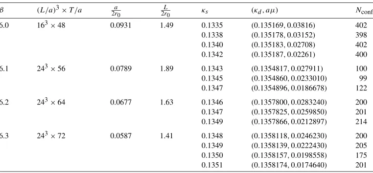
values of the lattice spacing in the rangea≈0.06–0.09 fm, with the spatial directions extending fromL≈1.4 to L≈1.9 fm. Time ranges fromx0=0 tox0=T, withT /L≈2.3–3.0. The three mass parameters (i.e. the standard hopping parameterκs for the strange quark, the twisted
hopping parameterκd and the twisted massμd for the down quark) are tuned as discussed in
Section2, so as to keep the two quarks degenerate. In order to avoid exceptional configurations in the untwisted strange sector, theK-meson mass is kept in the rangemK≈640–830 MeV; for
a discussion on the presence of exceptional configurations, seeAppendix D. The parameters of our runs are displayed inTable 1. Following Ref.[37], we will express our results in units of the length scaler00.5 fm. For the relationship betweenr0and the lattice couplingβ (which fixes
the lattice spacinga), seeAppendix A.
The effective pseudoscalar meson mass is computed from the ratio
(4.1)
aMPSeff(x0)=1
2ln
fAR(x0−a)−ifVR(x0−a)
fAR(x0+a)−ifVR(x0+a)
,
wherefAR,fVR are the correlation functions constructed from the improved operators of Eqs.
(2.30) and (2.31), giving results which are free ofO(a)effects at all times. In order to increase the signal stability, these correlation functions are antisymmetrised with their partnersfA
R and
fV
R.
[image:15.468.47.428.452.629.2]Flavour breaking effects have also been monitored by comparing the effective pseudoscalar meson mass of two axial correlation functions. The first is the quantity defined above, derived from the correlation function composed of a strange (standard Wilson) and a down (tmQCD
Table 1
The parameters of the runs at twist angleα=π/2 β (L/a)3×T /a 2ar
0
L
2r0 κs (κd, aμ) Nconf
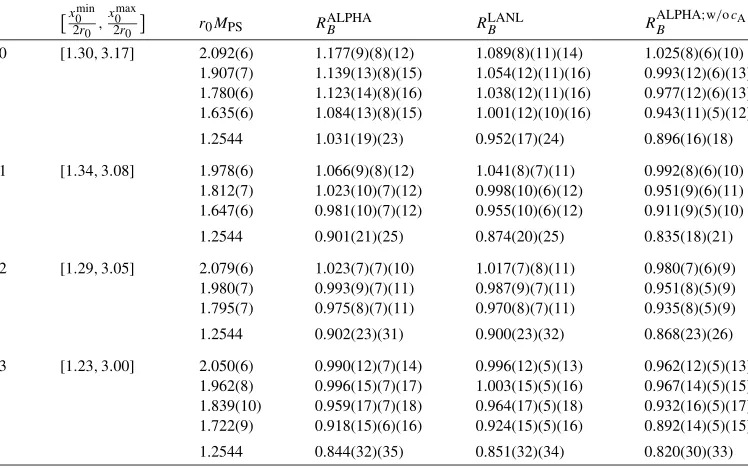
Table 2
Results for the pseudoscalar mass and the various ratios from whichBKis extracted (twist angleα=π/2). The error
inr0MPSis statistical. The three errors of theRBratio are, in order of appearance: (i) due to the statistical fluctuations
of the correlations; (ii) due to the errors ofZA,V; (iii) the total error from the two previous ones. The results of the extrapolations to the physical kaon mass values are shown at the bottom of eachβ-dataset: the first error ofRBis that
arising from type-(i) errors of the fitted values, while the second is from type-(iii) errors
β x
min 0
2r0 ,
xmax0
2r0
r0MPS RBALPHA RLANLB R
ALPHA;w/ocA
B
6.0 [1.30,3.17] 2.092(6) 1.177(9)(8)(12) 1.089(8)(11)(14) 1.025(8)(6)(10) 1.907(7) 1.139(13)(8)(15) 1.054(12)(11)(16) 0.993(12)(6)(13) 1.780(6) 1.123(14)(8)(16) 1.038(12)(11)(16) 0.977(12)(6)(13) 1.635(6) 1.084(13)(8)(15) 1.001(12)(10)(16) 0.943(11)(5)(12) 1.2544 1.031(19)(23) 0.952(17)(24) 0.896(16)(18) 6.1 [1.34,3.08] 1.978(6) 1.066(9)(8)(12) 1.041(8)(7)(11) 0.992(8)(6)(10)
1.812(7) 1.023(10)(7)(12) 0.998(10)(6)(12) 0.951(9)(6)(11) 1.647(6) 0.981(10)(7)(12) 0.955(10)(6)(12) 0.911(9)(5)(10) 1.2544 0.901(21)(25) 0.874(20)(25) 0.835(18)(21) 6.2 [1.29,3.05] 2.079(6) 1.023(7)(7)(10) 1.017(7)(8)(11) 0.980(7)(6)(9) 1.980(7) 0.993(9)(7)(11) 0.987(9)(7)(11) 0.951(8)(5)(9) 1.795(7) 0.975(8)(7)(11) 0.970(8)(7)(11) 0.935(8)(5)(9) 1.2544 0.902(23)(31) 0.900(23)(32) 0.868(23)(26) 6.3 [1.23,3.00] 2.050(6) 0.990(12)(7)(14) 0.996(12)(5)(13) 0.962(12)(5)(13)
1.962(8) 0.996(15)(7)(17) 1.003(15)(5)(16) 0.967(14)(5)(15) 1.839(10) 0.959(17)(7)(18) 0.964(17)(5)(18) 0.932(16)(5)(17) 1.722(9) 0.918(15)(6)(16) 0.924(15)(5)(16) 0.892(14)(5)(15) 1.2544 0.844(32)(35) 0.851(32)(34) 0.820(30)(33)
Wilson) quark propagators. The second is the effective mass derived from the fully twisted cor-relator, composed of an up and a down (tmQCD Wilson) quark propagator. As the twisted and untwisted quark flavours have been tuned to be degenerate in mass toO(a2)(cf. Section2.5), this is a measure of flavour breaking effects. The two effective masses computed from these cor-relation functions differ by∼5% atβ=6.0, while atβ=6.3 they practically coincide. Thus, small flavour breaking effects, visible at large lattice cutoffs, disappear as we move towards the continuum limit. Nevertheless, these effects require further and more detailed investiga-tion.
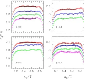
In order to determine the plateaux of the effective masses we have followed the procedure of Ref.[31]. We have allowed for a relative excited state contribution to the effective mass of at most 0.2% within the plateaux. The plateaux of the effective masses[x0min/r0, x0max/r0], which satisfy
this criterion, are listed inTable 2and illustrated inFig. 1. The values forx0min/r0indicate that the K-meson decay channel dominates the excited states after roughly 1.25–1.35 fm from thex0=0 wall source. The pseudoscalar meson massaMPSis obtained by averaging theaMPSeff(x0)values
in the plateaux; errors are estimated by the jackknife procedure, omitting one measurement from each bin. We present this result in the formr0MPSinTable 2.
Given these considerations, we determine BK by averaging in the symmetric interval
Fig. 1. Plateaux for the extraction ofMPSeffatα=π/2. The time-range and value of each plateau is indicated by a straight line segment.
(3.23)), corresponding to the bareBK.5We distinguish three sources of uncertainty in ourRB
results:
(i) The results depend on the prescription used for the determination of the normalisation con-stantsZAandZV, as well as the improvement coefficientcA. As discussed inAppendix A,
two such independent determinations have been provided by the ALPHA[38,39]and LANL
[40,41]Collaborations.6We compute the ratioRB for both sets of values. The discrepancy
between the two determinations is a measure ofO(a2)systematic effects. We also compute
RBwith the ALPHA Collaboration estimates forZAandZV, but without the improvingcA
counterterm in the axial current. Any discrepancy between this and the previous determina-tions ofRBsignals the presence of strongO(a)effects.
(ii) The statistical errors of the correlation functions are computed by a standard jackknife error analysis (omitting one measurement from each bin), without taking into account the errors ofZA,cAandZV.
5 Recall that the numerator ofR
Bis the bare correlation functionFVA+AVwhile the denominator is a properly nor-malised combination offAandfV. Also recall that the ratio is improved at tree level, and the denominator isO(a) improved in the chiral limit.
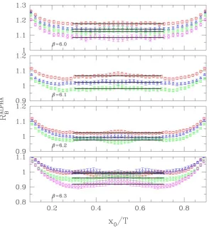
Fig. 2. Plateaux for the extraction ofRBALPHAatα=π/2. The time-range and value of each plateau is indicated by a
straight line segment.
(iii) The total statistical error is computed by combining the statistical errors ofZA,ZV (for a
given ALPHA or LANL determination) with those of the correlation functions, through the standard error propagation procedure. The statistical error ofcAis not taken into account, as
it is related to anO(a)correction (recall that for the same reason,cswis also used without an error).
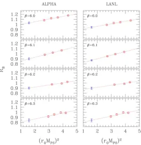
The results forRB (and pseudoscalar masses) are collected inTable 2. They have all been
computed at the time-plateaux shown in the second column, determined from the effective mass of Eq.(4.1)with ALPHA Collaboration values forZA,ZVandcA. The quality of the data is also
illustrated inFig. 2. It is clear that as the continuum limit is approached, theO(a2)discrepancies betweenRBALPHAandRLANLB tend to decrease. This tendency is less marked forRALPHA;w/ocA
B ,
which differs from the other two byO(a)effects.
TheRBvalues are extrapolated linearly in(r0MPS)2, to the physical point(r0MK)2=1.5736
(corresponding toMK2 =12[M2
K0+MK2±]), seeFig. 3. An interesting issue concerns the
magni-tude of the error of these extrapolated values. Usually, in quenched simulations performed at a givenβ, observables such as the ratioRBare computed on the same configuration ensemble for
Fig. 3. Linear extrapolation ofRBto the physical kaon mass atα=π/2.
Table 3
BK-parameter at fixed effective pseudoscalar massMPSefffor two different spatial lattice volumes (twist angleα=π/2). The various errors onRBare explained in the caption ofTable 2
L3×T /a4 r0MPS RALPHAB Nconf
163×48 1.635(6) 1.084(13)(8)(15) 400
243×48 1.624(5) 1.079(7)(8)(11) 167
the error of the extrapolation. We have instead opted for independent Monte Carlo simulations for each set of bare quark masses, which in this respect mimic unquenched simulations, at the price of having uncorrelatedRBresults with larger errors on the extrapolations.
The justification of the linear fit ofRB, as a function of the squared pseudoscalar mass is
provided inAppendix C.
4.1. Finite volume effects
In order to investigate finite volume effects, we have performed a simulation atβ=6.0 for a larger spatial volume, with extensionL/a=24, at the lightest massr0MPS=1.635. The results
are gathered inTable 3. Finite volume effects are estimated in terms of the following ratios:
(4.2)
MPS(L/a=16) MPS(L/a=24)−
1=0.007(5), R ALPHA
B (L/a=16)
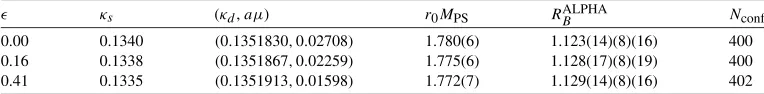
[image:19.468.49.429.415.455.2]Table 4
BK-parameter at fixed effective pseudoscalar massMPSefffor three values of the degeneracy-breaking parameter(twist angleα=π/2). The various errors onRBare explained in the caption ofTable 2
κs (κd,aμ) r0MPS RBALPHA Nconf
0.00 0.1340 (0.1351830,0.02708) 1.780(6) 1.123(14)(8)(16) 400 0.16 0.1338 (0.1351867,0.02259) 1.775(6) 1.128(17)(8)(19) 400 0.41 0.1335 (0.1351913,0.01598) 1.772(7) 1.129(14)(8)(16) 402
Note that all errors are of purely statistical nature. We see that the effective mass ratios have a very small statistical deviation from zero, while theBK ratio is essentially insensitive to finite
volume effects.
4.2. Non-degenerate masses
Past and current simulations for the determination ofBK have mostly been carried out with
degenerate down and strange quarks. The rationale behind this (at least as far as quenched sim-ulations are concerned) is to be found in the chiral perturbation theory expression forBK. As
discussed in Ref.[19–22], the quenched chiral expression forBKis given by
(4.3)
BK=B
1−3+2 ylny+by+cy2+δ
2−2
2 ln
1−
1+
+2
,
withy=m2K/(4π F )2andF 102 MeV (see Ref.[43]). The parameter
(4.4)
≡ms−md ms+md
is a measure of the down-strange degeneracy breaking. The expression(4.3)is identical in form to the one valid for dynamical quarks, save for theδ-term. This quenched artefact vanishes in the degenerate limit→0, but diverges when the down quark becomes chiral and→1.
We have measuredRBwith non-degenerate down and strange quarks. Our aim is to probe its
dependence on quark mass differences, while avoiding the potentially dangerous→1 limit. We have performed runs atβ =6.0, for two values of=0, tuning the bare mass parameters so that the pseudoscalar mass remains close to the valuer0MPS=1.780 of the=0 simulation.
Our results are summarised inTable 4. The effect of breaking the mass degeneracy of the valence quarks is estimated in terms of the following ratios:
(4.5)
MPS(=0)
MPS(=0.16)−1=0.003(5),
MPS(=0)
MPS(=0.41)−1=0.005(5),
(4.6)
RBALPHA(=0)
RALPHAB (=0.16)−1= −0.004(19),
RBALPHA(=0)
RBALPHA(=0.41)−1 = −0.005(17).
All errors are statistical. We see that there is no appreciable deviation between=0 and=0 values. It seems that, at least in the region of mass differences explored,BK is not sensitive to
the breaking of mass degeneracy.
K-meson of mK 650 MeV. This happened at β =6.0 and for a “standard” value of the
Wilson hopping parameter which, being generally considered “safe” from exceptional config-urations, has also been used in the simulations of other collaborations. More details are provided inAppendix D.
5. LatticeBK results from tmQCD atα=π/4
The quenchedBKparameter has also been computed in tmQCD with a twist angleα=π/4.
This formalism, with twisted down and strange quarks in the same flavour doublet, is a way to avoid the problem of exceptional configurations, while maintaining the property of multiplica-tive renormalisation of the four-fermion operator. Therefore, contrary to theα=π/2 simulation, in the present one it is possible to simulate at half the value of the physical strange quark mass directly, thus avoiding the uncertainties introduced by extrapolations from higher masses. The price to pay is that larger physical volumes are required at these smaller masses. Our simula-tions have been performed at four values of the lattice spacing in the rangea≈0.05–0.09 fm, while lattice spatial extensions areL≈1.9–2.2 fm. Time ranges fromx0=0 tox0=T, with T /L2. The two mass parameters (hopping parameterκ and twisted massμfor the two de-generate valence flavours) are tuned as discussed in Section2. Contrary to theπ/2 case, here we have generated a single configuration ensemble perβ, on which measurements at a few(κ, aμ)
values, tuned to be close to half the strange quark mass, are performed. The parameters of our runs are displayed inTable 5. We point out that at the smallest lattice spacing, corresponding to β=6.45, APEmille memory limitations made it impossible to maintain the physical vol-ume used at the lowerβ values. Consequently, in this case we were forced to run at a length of
L≈1.5 fm, with larger masses, and extrapolate to the pseudoscalar mass at the physical kaon mass.
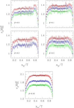
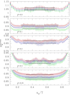
The effective pseudoscalar meson mass is computed from the ratio of Eq.(4.1); again correla-tion funccorrela-tions are antisymmetrised in time. The excited states analysis, carried out as in Ref.[44], determines the effective mass plateaux for which the relative contribution from the excited states is at most 0.5%. The plateaux of the effective masses[x0min/r0, x0max/r0]are listed inTable 6and illustrated inFig. 4. Once more, they have been obtained with the ALPHA Collaboration values forZA,ZVandcA. The quoted values forx0min/r0indicate that theK-meson channel dominates
the excited states after roughly 1.2 to 1.4 fm from the x0=0 wall source. The pseudoscalar
meson massaMPS is obtained by averaging the aMPSeff(x0) values in the plateaux; errors are
estimated by the jackknife procedure, omitting one measurement from each bin. This result is presented in the formr0MPSinTable 6.
The ratioRBis computed in the symmetric interval[x0min/r0, (T−x0min)/r0]. The results for RB are collected inTable 6. We see once more that as the continuum limit is approached, the O(a2)discrepancies betweenRBALPHAandRBLANLtend to decrease. This tendency is less marked forRALPHA;w/ocA
B , which differs from the other two byO(a)effects. The plateaux from which BK is extracted are illustrated inFig. 5.
TheRBvalues are interpolated linearly in(r0MPS)2, to the physical point(r0MK)2=1.5736,
Table 5
The parameters of the runs at twist angleα=π/4
β (L/a)3×T /a 2ar
0
L
2r0 (κ, aμ) Nconf
6.00 243×48 0.0931 2.24 (0.134739,0.010412) 200
(0.134795,0.009142) (0.134828,0.008397)
6.10 243×60 0.0789 1.89 (0.135152,0.00810) 200
(0.135190,0.00720) (0.135235,0.00615)
6.20 323×72 0.0677 2.17 (0.135477,0.007595) 73
(0.135539,0.006125)
6.30 323×72 0.0587 1.88 (0.135509,0.0076) 76
(0.135546,0.0067) (0.135584,0.0058)
6.45 323×86 0.0481 1.54 (0.135105,0.01459) 105
(0.135218,0.01185) (0.135293,0.01002)
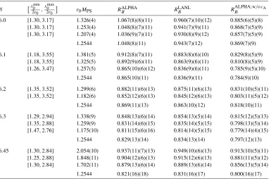
Table 6
Results for the pseudoscalar mass and the various ratios from whichBKis extracted (twist angleα=π/4). The error
inr0MPSis statistical. The three errors of theRBratio are, in order of appearance: (i) due to the statistical fluctuations
of the correlations; (ii) due to the errors ofZA,V; (iii) the total error from the two previous ones. The results of the extrapolations to the physical kaon mass values are shown at the bottom of eachβ-dataset: the first error ofRBis that
arising from type-(i) errors of the fitted values, while the second is from type-(iii) errors
β x
min 0
2r0 ,
xmax0
2r0
r0MPS RBALPHA RLANLB R
ALPHA;w/ocA B
6.0 [1.30,3.17] 1.326(4) 1.067(8)(8)(11) 0.960(7)(10)(12) 0.885(6)(5)(8)
[1.30,3.17] 1.253(4) 1.048(8)(7)(11) 0.941(7)(9)(11) 0.868(7)(5)(9)
[1.30,3.17] 1.207(4) 1.036(9)(7)(11) 0.930(8)(9)(12) 0.857(7)(5)(9) 1.2544 1.048(8)(11) 0.943(7)(12) 0.869(7)(9) 6.1 [1.18,3.55] 1.381(5) 0.912(8)(7)(11) 0.883(8)(6)(10) 0.829(8)(5)(9)
[1.18,3.55] 1.325(5) 0.892(9)(6)(11) 0.863(9)(6)(11) 0.810(8)(5)(9)
[1.26,3.47] 1.257(5) 0.865(10)(6)(12) 0.836(9)(6)(11) 0.785(9)(5)(10) 1.2544 0.865(10)(11) 0.836(9)(11) 0.784(9)(10) 6.2 [1.35,3.52] 1.299(6) 0.882(11)(6)(13) 0.875(11)(6)(13) 0.831(10)(5)(11)
[1.35,3.52] 1.182(6) 0.852(12)(6)(13) 0.845(12)(6)(13) 0.803(11)(5)(12) 1.2544 0.869(11)(13) 0.863(10)(12) 0.818(10)(11) 6.3 [1.29,2.94] 1.338(9) 0.848(13)(6)(14) 0.854(13)(5)(14) 0.815(12)(5)(13)
[1.35,2.88] 1.259(9) 0.831(14)(6)(15) 0.835(14)(5)(15) 0.798(13)(5)(14)
[1.47,2.76] 1.175(10) 0.811(15)(6)(16) 0.814(14)(5)(15) 0.779(14)(4)(15) 1.2544 0.829(13)(14) 0.834(13)(14) 0.797(12)(13) 6.45 [1.30,2.84] 2.054(10) 0.937(11)(7)(13) 0.949(10)(6)(13) 0.913(10)(5)(11)
[1.25,2.88] 1.848(11) 0.904(12)(6)(13) 0.915(12)(6)(13) 0.881(11)(5)(12)
[image:22.468.42.424.374.628.2]Fig. 4. Plateaux for the extraction ofMPSeffatα=π/4. The time-range and value of each plateau is indicated by a straight line segment.
5.1. Finite volume effects
In order to test finite volume effects, we have performed simulations atβ=6.0,6.1,6.2 for various spatial volumes and light quark masses. The simulation points, as well as the results for the pseudoscalar meson mass and forRB, are gathered inTable 7. The spatial extent of the
Fig. 5. Plateaux for the extraction ofRBALPHAatα=π/4. The time-range and value of each plateau is indicated by a
straight line segment.
different spatial volumes are computed at fixedβ and their deviation from unity is presented in
Table 8.
Forβ =6.0,6.1 the effective mass ratios display some small finite volume effects, atL∼
1.5 fm to 2 fm, which appear to vanish atL∼2.5 fm. Forβ=6.2 however, such effects are also absent already atL∼1.5 fm. It has to be noted that at this level of precision it is difficult to disentangle finite volume effects from e.g. the difference in cutoff effects, or the systematic uncertainties related to excited states.
ForBKwe see finite volume effects atL∼1.5 fm, which disappear atL∼2 fm. This situation
Fig. 6. Linear inter/extrapolation ofRBto the physical kaon mass atα=π/4.
6. BKin the continuum limit
Having obtained the value of the bareBK parameter at several lattice spacings, we now
pro-ceed to the computation of its renormalised counterpart in the continuum limit. In Ref.[13], the necessary renormalisation constants have been calculated non-perturbatively in various Schrödinger functional schemes, as well as the operator step scaling functions, which determine its renormalisation group running. What we need from Ref. [13] is the total renormalisation factorZVA++AV;(g0), which connects the bareBKto its RGI value as follows:
(6.1)
ˆ
BK= lim g0→0
ZVA++AV;s(g0)BK(g0).
The bare BK(g0)is given by RB at the physical pointr0MK (seeTables 2 and 6). Which of
the three candidatesRBALPHA,RBLANLorRALPHA;w/ocA