Evolutionary MPNN for Channel Equalization
Archana Sarangi
1, Bijay Ketan Panigrahi
2& Siba Prasada Panigrahi
31Department of AEIE, ITER, SOA University, Bhubaneswar, India; 2Department of Electrical Engineering, IIT, Delhi, India; 3 Depart-ment of Electrical Engineering, KIST, Bhubaneswar, India
Email: [email protected]
Received December 10th, 2010; revised January 11th, 2011; accepted February 18th, 2011
ABSTRACT
This paper proposes a novel equalizer, termed here as Evolutionary MPNN, where a complex modified probabilistic Neural Networks (MPNN) acts as a filter for the detected signal pattern. The neurons were embedded with optimization algorithms. We have considered two optimization algorithms, Bacteria Foraging Optimization (BFO) and Ant Colony Optimization (ACO). The proposed structure has the ability to process complex signals also can perform for slowly varying channels. Also, Simulation results prove the superior performance of the proposed equalizer over the existing MPNN equalizers.
Keywords: Channel Equalization, Probabilistic Neural Network, Bacteria Foraging, Ant Colony Optimization
1. Introduction
Channel equalization plays an important role in digital communication systems. There are tremendous devel-opments in equalizer structures since the advent of neural networks in signal processing applications. Recent lite-rature is healthy enough with newer applications of neural networks [1-5] and in particular to independent component analysis, noise cancellation and channel equalization [6-16]. But all of these papers overlooked two basic problems encountered. First is to train the equalizer how to process complex signal. Second is to get a adaptive nature of equalizer for slowly varying channels. Authors in [17] have tried to address these two problems, through a Modified Probabilistic Neural net-work (MPNN), and were successful to process complex signals and for a slowly varying signal. However, the result was sub-optimal in nature, since the neurons were not trained with any optimization algorithms.
This paper takes the similar structure as that of [17]. But, novelty in this paper is to use the structure as a neural filter for classifying detected signal pattern. Neu-rons in network in [17] were embedded with stochastic gradient, whereas in this paper, each of the neurons in the structure is embedded with optimization algorithm unlike that of in [17].
Recently, Particle Swarm Intelligence (PSO) [18], Bacteria Foraging Optimization (BFO) [19-21] and Ant colony Optimization (ACO) [22-26] have been used for optimization purpose in different fields of research. This
paper uses BFO and ACO for optimization. Some suc-cessful applications of these two techniques, i.e. BFO and ACO can be found in [27-31]. Novelty in this paper can be seen as, application of two known algorithms, ACO and BFO, to the problem of channel equalization. This underlines the improvement added by the optimiza-tion algorithms. The proposed schemes outperform the existing equalizers.
2. Problem Statement
Impulse response of channel & co-channel can be represented as:
( )
1 , 00
i
p
j
i i j
j
H z a z i n
− − =
=
∑
≤ ≤ (1)Here piand ai j, are length and tap weights of ith
channel impulse response. We assume a binary commu-nication system, which would make the analysis simple, though it can be extended to any communication system in general. The transmitted symbols x ni
( )
, 0≤ ≤i nfor channel and co-channel are drawn from a set of in-dependent, identically distributed (i.i.d) dataset compris-ing of {± 1} and these are mutually independent. This satisfies the condition
( )
0i
E x n = (2)
( ) ( )
1 2(
) (
1 2)
i j
E x n x n = δ i− j δ n −n (3)
( )
1 00 0
n n
n
δ = =
≠
(4)
The channel output scalars can be represented as
( )
( )
co( ) ( )
y n =d n +d n +η n (5) Here d n
( )
desired received signal dco( )
n is inter-fering signal and η( )
n is noise component assumed to be Gaussian with variance E 2( )
n 2η
η σ
=
and
uncor-related with data. The desired and interfering signal can be represented as
( )
0 1(
)
0, 0 0 p
j j
d n a x n j
− =
=
∑
− (6)( )
1 ,(
)
1 0
i
p n
co i j i
i j
d k a x n j
− = =
=
∑ ∑
− (7)The task of the equalizer is to estimate the transmitted sequence x0
( )
n−dˆ based on channel observation vector( )
( ) (
, 1 ,)
,(
1)
Ty n =y n y n− y n m− + , where m is
order of equalizer and dˆ is decision delay.
The cost function is the MSE value of e p q n
(
, , +1)
. So(
)
2 1
, , 1
2
J= e p q n+ (8)
The error generated at the output of equalizer should be minimized to give an acceptable solution. The initial condition for the equalizer model is derived from the Decision Feedback Equalization (DFE) expressions. So, determination of the error at interior points the channel is essential. This paper assumes, input same as that of de-sired output. Hence, the total error is the difference between output and input of the network model. The cost function is the mean of the sum of squares of this error (MSE).
3. Proposed Equalizer
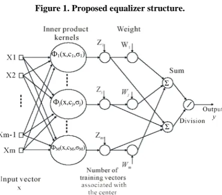
The proposed equalizer in this paper shown in Figure 1 and consists of two basic components, one MPNN filter and one optimizer. The purpose of filter is to receive the distorted output from the channel and will form two separate and independent patterns, one for
{ }
+1 and next for{ }
+1 . The purpose of the optimizer is to optim-ize the cost function of (8) and thereby minimizing the error. The details of classifier and working algorithms for the optimizer are discussed in following two sub- sections.3.1. MPNN Filter
First part of the equalizer of this paper, the filter, shown in Figure 2, is the same structure as that used in [17]. Authors in [17] used the structure for the purpose of equalization without any evolutionary optimizing algo-rithms. Authors in [17], embedded stochastic gradient to
neural nets. But, in this paper we have embedded opti-mization algorithm to neural network. This optiopti-mization algorithm is however, shown separately in the equalizer structure and also discussed separately in following sub-section.
The MPNN structure is based on Nadaraya-Watson Regression estimator [17] given by:
(
)
(
(
) (
)
)
(
) (
)
(
)
2 1
2 1
exp 2
ˆ
exp 2
T n
k k k
k
T n
k k
k
y x x x x
E Y X
x x x x
σ σ
= =
− − −
=
− − −
∑
∑
(9)Here, x is input sample. Each training input sample, ; 1, 2,
k
x k= n, form a center in the input space. An input vector to be evaluated xt is weighted exponen-tially according to its Euclidean distance from the centers. The corresponding observed output from each center,
k
y , is averaged to give the estimate E Y Xˆ
(
)
. The val-ue of σ determines how the network behaves.In general, σ governs the “closeness” between a point of interest, say xt, and the centers, x kk; =1, 2,n, in the input space.
For a small σ value, only the corresponding observed values, yk:k=a, of the closest center, (xk:k=a)
appear significant, compare to the contribution from oth-er centoth-ers, (yk :k=1,n k, ≠a). In this case, the net-work does the nearest neighbor search. With a larger
[image:2.595.313.536.510.706.2]σ value, more of the observed outputs, yk, are taken into account, but with those corresponding to centers close to xt being given more weight.
Figure 1. Proposed equalizer structure.
Ф1(x,c1,σ1)
Фj(x,cj,σj)
ФM(x,cM,σM)
Σ
Σ
This MPNN structure will be able to process complex m-dimensional input vectors and complex outputs im-plementing a mapping f C: N →C [17], if equation (9) can be written as:
(
)
(
(
) (
)
)
(
) (
)
(
)
2 1
2 1
exp 2
ˆ
exp 2
H M
i i i i
i
H M
i i i
i
Z y x c x c
E Y X
Z x c x c
σ σ
= =
− − −
=
− − −
∑
∑
(10)where
( )
⋅H denotes Hermitian operator (or conjugate transpose). Zi, is the number of input training vector associated with center ci.3.2. The Optimizer
Second part of the equalizer proposed in this paper is an optimizer. However, practically, one optimization algo-rithm, which is discussed in this section, is embedded to the neural network that is used as a filter. Embedding neurons with optimization algorithms is achieved through training the neurons for these algorithms like that in [13,27]. We have taken two different optimization algorithms, first one Bacteria foraging optimization and next with Ant colony optimization. The algorithms are discussed in following sections, and for clarity of the readers, with different nomenclatures. This paper has not tested the structure with any other optimization algo-rithms and can be seen as one area for future work.
3.2.1. Bacteria Foraging Optimization
Natural selection tends to eliminate animals with poor foraging strategies and favor the propagation of genes of those animals that have successful foraging strategies, since they are more likely to enjoy reproductive success. After a number of generations, poor foraging strategies are either eliminated or shaped into good ones. This ac-tivity of foraging led the researchers to use it as optimi-zation process. The E. coli bacteria that are present in our intestines also undergo a foraging strategy. The control system of these bacteria that dictates how foraging should proceed can be subdivided into four sections, namely, chemo taxis, swarming, reproduction, and elimination and dispersal. We will use following nomenclature for dif-ferent parameters of BFO.
S: Number of bacteria to be used for searching the total region:
is
N : Number of input sample
p: Number of parameter to be optimized
s
N : Swimming length after which tumbling of bacte-ria will be undertaken in a chemotactic loop
c
N : Number of iterations to be undertaken in a che-motactic loop. Always
re
N : Maximum number of reproduction to be under-taken
ed
N : Maximum number of elimination and dispersal
events to be imposed over the bacteria.
ed
P : Probability with which the elimination and dis-persal will continue.
( )
C i : Run length unit
For initialization, we must choose P S N N N, , c, s, re, ,
ed ed
N P and the C i i
( )
, =1, 2,S. In case of swarming, we will also have to pick the parameters of the cell-to-cell attractant functions; here this paper uses the parameters given above. Also, initial values for the θi,i=1, 2,Smust be chosen. Choosing these to be in areas where an optimum value is likely to exist is a good choice. Alter-natively, we may want to simply randomly distribute them across the domain of the optimization problem. The al-gorithm that models bacterial population chemo taxis, swarming, reproduction, elimination, and dispersal is given here (initially, j= = =k l 0). For the algorithm, note that updates to the θiautomatically result in updates to P. Clearly, we could have added a more sophisticated termination test than simply specifying a maximum number of iterations.
Elimination-dispersal loop: l= +l 1
Reproduction loop: k= +k 1
Chemo taxis loop: j= +j 1
For i=1, 2,S take a chemo tactic step for bacte-rium i as follows.
Compute J i j k l
(
, , ,)
(i.e., add on the cell-to-cell at-tractant effect to the nutrient concentration).Let Jlast =J i j k l
(
, , ,)
to save this value since we may find a better cost via a run.Tumble: Generate a random vector ∆
( )
i ∈RP with each element ∆m( )
i m, =1, 2,,p, a random number on [–1, 1].Move
(
)
(
) ( ) ( )
( ) ( )
11, , , ,
i i
t
j k l j k l c i i
i i
θ + =θ + ∆
∆ ∆ This
results in a step of size c i
( )
in the direction of the tum-ble for bacteriumi
.Compute J i j
(
, +1, ,k l)
and then let,(
)
(
)
(
(
) (
)
)
, 1, ,
, 1, , cc i 1, , . 1, ,
J i j k l
J i j k l J θ j k l P j k l
+ =
+ + + +
Swim (note that we use an approximation since we de-cide swimming behavior of each cell as if the bacteria numbered
{
1, 2i}
have moved and{
i+1,i+2s}
have not; this is much simpler to simulate than simulta-neous decisions about swimming and tumbling by all bacteria at the same time):
Let m=0 (counter for swim length).
While m<Ns (if have not climbed down too long) Let m= +m 1
Let Jlast =J i j
(
, +1, ,k l)
and let(
)
(
) ( ) ( )
( ) ( )
11, , , ,
i i
t
j k l j k l c i i
i i
θ + =θ + ∆
∆ ∆ and
use this i
(
1, ,)
j k l
θ + to compute new J i j
(
, +1, ,k l)
as we did in above step.
Else, let m=Ns this is the end of the while statement.
Go to next bacterium
(
i+1)
if i≠S (i.e., go to b) to process the next bacterium).If j≤Nc, go to step 3. In this case, continue chemo taxis, since the life of the bacteria is not over.
Reproduction:
For the given k and l, and for each i=1, 2,Slet
(
)
1
1 , , ,
c N i
health j
J =
∑
=+ j i j k l be the health of bacteriumi
(ameasure of how many nutrients it got over its lifetime and how successful it was at avoiding noxious substances) Sort bacteria and chemo tactic parameters c i
( )
in order of ascending cost Jhealth (higher cost means lower health). The Sr bacteria with the highest Jhealth values die and the other Sr bacteria with the best values split (and the copies that are made are placed at the same location as their parent).If K≤Nre go to step 2. In this case, we have not reached the number of specified reproduction steps, so we start the next generation in the chemo tactic loop.
Elimination-dispersal: for i=1, 2,S, with probabil-ity Ped, eliminate and disperse each bacterium (this keeps the number of bacteria in the population constant). For doing this, if we eliminate a bacterium, simply disperse one to a random location on the optimization domain.
If I≤Ned then go to step 1; otherwise end. 3.2.2. Ant Colony Optimization
Ant colony optimization (ACO) is a population-based search technique working constructively to solve opti-mization problems by using principle of pheromone in-formation. This is an evolutionary approach where several generations of artificial agents in a cooperative way search for good solutions. These agents are initially ran-domly generated on nodes, and stochastically move from a start node to feasible neighbor nodes. While in the process of finding feasible solutions, agents collect and store information in pheromone trails. Agents can release pheromone online while building solutions. Also, the pheromone will be evaporated in the search process to avoid local convergence and to explore more search areas. Then after, additional pheromone is deposited to update pheromone trail offline so as to bias the search process in favor of the currently optimal path. The pseudo code of ant colony optimization is stated as [20]:
Procedure: Ant colony optimization (ACO) Begin
While (ACO has not been stopped) do Agents_generation_and_activity(); Pheromone_evaporation(); Daemon actions(); End;
End;
In this ACO, agents find solutions starting from a start node and moving to feasible neighbor nodes in the process of Agents_generation_and_activity. While in the process, information collected by agents is stored in the so-called pheromone trails. In this process, agents can release pheromone along with building the solution (online step-by-step) or while the solution is built (online de-layed). An agent-decision rule, made up of the pheromone and heuristic information, governs agents_ search toward neighbor nodes stochastically. The kth ant at time
t
po-sitioned on node r move to the next nodes
with the rule governed by( )
( )
{
}
0arg max
k ru ru
u allowed t t when q q
s
S otherwise
α β
τ η
=
≤
=
(15)
where τru
( )
t is the pheromone trail at time t, ηru is the problem-specific heuristic information, a is a para-meter representing the importance of pheromone infor-mation, β is a parameter representing the importance of heuristic information, q is a random number uniformly distributed in [0, 1], q0 is a pre-specified parameter (0≤q0≤1), allowedk(t) is the set of feasible nodescur-rently not assigned by ant k at time t, and S is an index of node selected from allowedk(t) according to the probability distribution given by
( )
( )
( )
( )
( )
0
k
rs rs
k k
rs ru rs
u allowed t
t
if s allowed t t
P t
otherwise
α β
β
τ η
τ η
∈
∈
=
∑
(16)Pheromone_evaporation is a process of decreasing the intensities of pheromone trails over the course of time. This process has been used to avoid locally convergence and to explore more search space. Daemon actions may or may not be used in ant colony optimization, and they are often used to collect useful global information by depositing additional pheromone. In the original algo-rithm of [20], there is a scheduling process for the above three processes. This is to provide freedom for conduct-ing how these three processes should interact in ant co-lony optimization and other approaches.
4. Simulation Results
symmetric channel impulse response with an impulse response considered as:
( )
1 20.2887 0.9129 0.2887
H z = + z− + z− (9)
Transmitted signal constellation was set to {± 1} keeping the transmitted power unity. Co-channel Inter-ference was treated as noise. For simulation the training data consisted of 8 random values of p, and 25 random values of n (including n=0, and n=256).
For the simulations, optimization parameters chosen as:
8
S = ; Nis =100; p=8; Ns=3; Nc =5;
30
re
N = ; Ned =10; Ped =0.25; C i
( )
=0.075For the simulations, we considered three cases. In first case, detected signal was feedback to classifier for weight updating of neurons similar to that in [1]. In second case, detected signal was optimized with BFO and send back to classifier as feedback signal for updat-ing the neurons. In third case, detected signal was opti-mized with ACO and send back to classifier as feedback signal for updating the neurons. Figures 2 and 3 respec-tively shows Mean square Error (MSE) and Symbol Er-ror Rate (SER) curves for these three cases.
From Figure 3, it is clear that Mean square Error (MSE) is much lower for BFO trained MPNN than that of MPNN [17]. Where as, ACO trained MPNN performs almost similar to that of MPNN of [17].
From Figure 4, it is shown that Equalizer with an op-timizer outperforms the equalizer [17] without opop-timizer. Also it is interesting to see the comparison between two optimization strategies used. Here BFO performs better than ACO.
Figure 3. MSE for MPNN [17], BFO trained and ACO trained equalizer.
[image:5.595.309.535.86.263.2]Figure 4. SER for MPNN [17], BFO trained and ACO trained equalizer.
Table 1. Computational Complexity of different equalizers.
Equalizer Additions Multiplications
MPNN N M
MPNN trained
with ACO N + M/2 N/2 + M MPNN trained
with BFO 1.6 N 2 M
Though the proposed equalizer outperforms MPNN equalizer without optimization, but with affordable in-crease in computational complexities. This is because of accommodating the optimization algorithms. Table 1 compares this having MPNN as base. It is also seen that though BFO performs better than ACO, comes with larger complexity.
5. Conclusions
This paper proposed a novel equalizer where a hybrid structure of two multi-layer neural networks acts as a classifier to classify the detected signal pattern. The neurons were embedded with optimization algorithms. Simulation results prove the superior performance ofthe proposed equalizer. Works reported in this paper can also be extended to other optimization algorithms like PSO, DEPSO etc, also can be tested with hybrid algorithms developed using BFO, ACO, PSO etc.
REFERENCES
[1] E. D. Übeyli, “Lyapunov Expoents/Probabilistic Neural Networks for Analysis of EEG Signals,” Expert Systems with Applications, Vol. 37, No. 2, 2010, pp. 985-992.
[image:5.595.310.537.322.402.2] [image:5.595.60.284.512.692.2]
Lyapunov Exponents for Analysis of ECG Signals,” Ex-pert Systems with Applications, Vol.37,No.2, 2010, pp.
1192-11
[3] D.-T. Lin, et al., “Trajectory Production with Adaptive Time-Delay Neural Network,” Neural Networks, Vol.8,
No. 3, 1995, pp. 447-461.
[4] L. Gao and S. X. Ren, “Combining Orthogonal Signal Correction and Wavelet Pocket Transform with Radial Basis Function Neural Networks for Multicomponent Determination,” Chemometrics and Intelligent Laborato-ry Systems, Vol. 100, No. 1, 2010, pp. 57-65.
[5] K.-L. Du, “Clustering: A Neural Network Approach,”
Neural Networks, Vol. 23, No. 1, 2010, pp. 89-107.
[6] H. Q. Zhao, et al., “Adaptive Reduced Feedback FLNN Filter for Active Control of Noise Processes,” Signal Processing, Vol. 90, No. 3, 2010, pp. 834-847.
[7] C. Potter, et al., “RNN Based MIMO Channel Predic-tion,” Signal Processing, Vol.90, No. 2, 2010, pp. 440-
450
[8] J. C. Patra, et al., “Nonlinear Channel Equalization for Wireless Communication Systems Using Legendre Neur-al Networks,” Signal Processing, Vol.89, No.11, 2009,
pp.2251-2262.
[9] S. P. Panigrahi, et al., “Hybrid ANN Reducing Training Time Requirements and Decision Delay for Equalization in Presence of Co-Channel Interference,” Applied Soft
Computing, Vol. 8, No. 4, 2008, pp. 1536-1538.
[10] L. Zhang and X. D. Zhang, “MIMO Channel Estimation and Equalization using Threelayer Neural Network with Feedback,” Tsinghua Science & Technology, Vol.12, No.
6, 2007, pp.658-662.
[11] H. Q. Zhao and J. S. Zhang, “Functional Link Neural NetWork Cascaded with Chevyshev Orthogonal Poly-nomial for Nonlinear Channel Equalization,” Signal Processing, Vol. 88, No. 8, 2008, pp. 1946-1957.
[12] H. Q. Zhao and J. S. Zhang, “A Novel Nonlinear Adap-tive Filter using a Pipelined Second-Order Volterra Re-current Neural Network,” Neural Networks, Vol.22, No. 10, 2009, pp. 1471-1483.
[13] W.-D. Weng, et al., “A Channel Equalizer Using Re-duced Decision Feedback Chebyshev Functional Link Artificial Neural Networks,” Information Sciences, Vol. 177,No.13, 2007, pp.2642-2654.
[14] W. K. Wong and H. S. Lim, “A Robust and Effective Fuzzy Adaptive Equalizer for Powerline Communication Channels,” Neurocomputing, Vol.71,No. 1-3, 2007, pp.
311-322.
[15] J. Lee and R. Sankar, “Theoretical Derivation of
Mini-mum Mean Square Error of RBF based Equalizer,” Sig-nal Processing, Vol. 87,No.7, 2007, pp. 1613-1625.
[16] H. Q. Zhao and J. S. Zhang, “Nonlinear Dynamic System Identification Using Pipelined Functional Link Artificial Recurrent Neural Network,” Neurocomputing, Vol. 72, No.13-15, 2009, pp. 3046-3054.
[17] S. K. Padhy, et al., “Non-Linear Channel Equalization using Adaptive MPNN,” Applied Soft Computing, Vol.9,
No. 3, 2009, pp.1016-1022.
[18] M. A. Guzmán, et al., “A Novel Multiobjective Optimi-zation Algorithm based on Bacterial Chemotaxis,” Engi-neering Applications of Artificial Intelligence, Vol. 23,
No. 3, 2010, pp.292-301.
[19] B. Majhi and G. Panda, “Development of Efficient Iden-tification Scheme for Nonlinear Dynamic Systems using Swarm Intelligence Techniques,” Expert Systems with Applications, Vol. 37, No. 1, 2010, pp. 556-566.
[20] D. P. Acharya, G. Panda and Y. V. S. Lakshmi, “Effects of Finite Register Length on Fast ICA, Bacteria Foraging Optimization Based ICA and Constrained Genetic Algo-rithm based ICA AlgoAlgo-rithm,” Digital Signal Processing, Available Online, August 2009.
[21] B. K. Panigrahi and V. Ravikumar Pandi, “Congestion Management Using Adaptive Bacterial Foraging Algo-rithm,” Energy Conversion and Management, Vol. 50, No. 5, 2009, pp. 1202-1209.
[22] M. Korürek and A. Nizam, “Clustering MIT-BIH Arr-hythmias with Ant Colony Optimization using Time Do-main and PCA Compressed Wavelet Coefficients,” Digi-tal Signal Processing, Available online 13 November 2009.
[23] M. H. Aghdam, et al., “Text Feature Selection Using Ant Colony Optimization,” Expert Systems with Applications, Vol. 36, No. 3, 2009, pp. 6843-6853.
[24] S.-S. Weng and Y.-H. Liu, “Mining Time Series Data for Segmentation by Using Ant Colony Optimization,” Eu-ropean Journal of Operational Research, Vol. 173, No. 3, 2006, pp. 921-93 [25] J. Tian, et al., “Ant Colony Optimization for Image
Shrinkage,” Pattern Recognition Letters, Available on line 7 January, 2010.
[26] W. Chen, N. Minh and J. Litva, “On Incorporating Finite Impulse Response Neural Network with Finite Difference Time Domain Method for Simulating Electromagnetic Problems,” Antennas and Propagation Society Interna-tional Symposium, Vol. 3, 1996, pp. 1678-1681.
[28] D. H. Kim, A. Abraham, and J. H. Cho, “A Hybrid Ge-netic Algorithm and Bacterial Foraging Approach for Global Optimization,” Information Sciences, Vol. 177, No. 18, 2007, pp. 3918-3937.
[29] A. Biswas, S. Dasgupta, S. Das and A. Abraham, “Syn-ergy of PSO and Bacterial Foraging Optimization — A Comparative Study on Numerical Benchmarks,” Innova-tions in Hybrid Intelligent Systems, Vol. 44, 2007, pp. 255-2
[30] C. Grosan and A. Abraham, “Hybrid Evolutionary Algo-rithms: Methodologies, Architectures, and Reviews,”
Hybrid Evolutionary Algorithms, Vol. 75, 2007, pp. 1-17.
[31] H. Chen, Y. L. Zhu, K. Y. Hu, “Multi-Colony Bacteria Foraging Optimization with Cell-to-Cell Communication for RFID Network Planning,” Applied Soft Computing, Vol. 10, No. 2, 2010, pp. 539-547.
![Figure 4. SER for MPNN [17], BFO trained and ACO trained equalizer.](https://thumb-us.123doks.com/thumbv2/123dok_us/9012125.397903/5.595.60.284.512.692/figure-ser-mpnn-bfo-trained-aco-trained-equalizer.webp)
