Recognition Method of Multidimensional Poverty Based on Mahalanobis Taguchi System

ISSN Online: 2327-5960 ISSN Print: 2327-5952

DOI: 10.4236/jss.2019.78012 Aug. 20, 2019 161 Open Journal of Social Sciences

Recognition Method of Multidimensional

Poverty Based on Mahalanobis-Taguchi System

Wenhe Chen

, Zhipeng Chang

1_{School of Business, Anhui University of Technology, Maanshan, China}

2_{Institute of Anhui’s Innovation Driving and Development, Anhui University of Technology, Maanshan, China}

Abstract

This paper recognizes multidimensional poverty in rural China using the Mahalanobis-Taguchi System on the China Labor-force Dynamic survey (CLDS) 2014 dataset. Six dimensions are included: Income, Education, health, living, asset and housing. Results suggest that the MTS can precisely recognize poor and non-poor households and select the main indexes leading to multidimensional poverty. Enhancing income and improving farming effi-ciency are the main means of poverty reduction. Moreover, improving rural living and health conditions by strengthening public services and infrastruc-ture should also be a policymaking concern.

Keywords

Mahalanobis-Taguchi System, Rural Families, Multidimensional Poverty, Precise Recognition

1. Introduction

Poverty is not only a common challenge to humankind but also an important issue for China’s economic and social development. Sen (1976) believes that po-verty leads to the lack and deprivation of capacity, which can reduce the oppor-tunities for the poor population to gain income growth and get out of poverty [1]. In addition, World Bank (2001) points out that poverty in China causes the absence of education, health, and nutritional aspects prevail, which hinders the development of China’s society [2]. Since the launch of the ‘‘Reform and Open-ing Up’’ in 1978, China has made significant progress in poverty alleviation. However, the marginal benefit of poverty alleviation decreases year by year. By 2018, there are still 16.6 million poor people in rural China, and there are many difficulties in poverty alleviation. In the context of large data, the appropriate

How to cite this paper: Chen, W.H. and Chang, Z.P. (2019) Recognition Method of Multidimensional Poverty Based on Maha-lanobis-Taguchi System. Open Journal of Social Sciences, 7, 161-174.

https://doi.org/10.4236/jss.2019.78012

Received: July 23, 2019 Accepted: August 17, 2019 Published: August 20, 2019

Copyright © 2019 by author(s) and Scientific Research Publishing Inc. This work is licensed under the Creative Commons Attribution International License (CC BY 4.0).

DOI: 10.4236/jss.2019.78012 162 Open Journal of Social Sciences poverty recognition method can provide methodological support for poverty al-leviation in poor areas.

Poverty has traditionally been seen as lacking income (or consumption). However, over the past 40 years, this multidimensional concept of poverty has been queried, and Scholars tend to analyze the poverty from a multi-dimensional perspective, according to the seminal works of Sen (1976) [1]. From this pers-pective, income is not the only indicator of poverty. The reasons are mainly re-flected in two aspects. On the one hand, existing studies have shown that there are often high tolerance and exclusion errors between people with low incomes and those deprived of other aspects of human well-being (Baulch and Maasset 2003; Ruggeri Laderchi et al. 2003) [3][4]. On the other hand, the disadvantage of the monetary-metric income approach is that not all non-monetary characte-ristics can be directly measured. The reason is that the markets do not work well in many developing countries (Bourguignon and Chakravarty 2003) [5]. There-fore, although income is a significant dimension to evaluate human develop-ment, other dimensions should be considered to measure human deprivation such as education, living standards, health, and assets. Multidimensional poverty measurement and recognition have been the main research direction since its conceptual foundation was put forward by Sen. A variety of multidimensional poverty measurement methods were proposed. For example, Hagenaars et al. (1987) constructed the multi-dimensional poverty index system from the two dimensions of leisure and income [6]. Lugo et al. (2009) built a multidimension-al poverty measurement model based on information theory [7]. Tsui (2002) and Bourguignon (2003) used axiomatic methods to measure the multi-dimensional poverty index [8][9]. Alkire (2011) put forward the AF method based on axi-omatization [10]. The core of the AF method is the “double critical value” me-thod. First, the critical value of each index is used to judge whether the object is deficient in this dimension; Then, the critical value of all dimensions is estab-lished to judge whether the individual belongs to multidimensional poverty. However, this method belongs to the unitary statistical method, which is essen-tially an extension of the analysis method of one-dimensional poverty. It can only examine the contribution of a single dimension to the multi-dimensional poverty, and cannot recognize the poor households from a multidimensional perspective.

DOI: 10.4236/jss.2019.78012 163 Open Journal of Social Sciences propose a recognition method of multidimensional poverty based on MTS.

2. Mahalanobis-Taguchi System

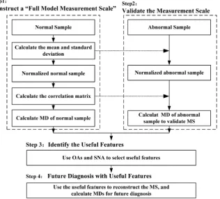
MTS is a pattern recognition method developed by Dr. Taguchi, which is applied to classify data and select useful features. MTS is composed of MD and Taguchi’s Robust Engineering. MD is a covariance distance used to measure the similari-ties between unknown and known sample sets, which is used to construct a measurement scale to recognize samples in multidimensional systems. Taguchi method is a statistical method to improve engineering quality (Taguchi, 2007) [15] and enhance system robustness (Taguchi, 2001) [10]. This study uses MTS to select useful features of multidimensional poverty and recognize poor house-holds. There are four steps in MTS, as shown in Figure 1.

Step 1: Construct a “Full Model Measurement Scale” with MS as the Ref-erence

In this stage, we collect sample data from the non-poor families to construct the normal sample dataset. Moreover, their MDs are used to construct the Ma-halanobis Space (MS), which are around one.MS can be considered a database for the normal dataset, combining its mean vector, standard deviation vector, and covariance matrix. Ordinarily, the samples in the normal group should be similar and have common characteristics. We use the mean point and the aver-age MD of the normal group for serving as the reference point and the base of the measurement scale.

DOI: 10.4236/jss.2019.78012 164 Open Journal of Social Sciences We assume t items

(

)

mul-tidimensional poverty. We first collect n normal samples with p features to con-struct an MS as a reference, where xitis the original value of tth feature of the ith normal sample. Standardization of each feature using the mean xt and

stan-dard deviation st is essential because features have different measurement scales, the equitation as follows:

it t it t x x z s −

= ₍₁₎

where, 1 1 n t it i x x n =

=

∑

(

)

1 1

1

n

t it t

i

s x x

n =

= −

−

∑

After standardization, The mean and standard deviation of each feature are 1 and 0. the correlation matrix C is computed by the equation as below:

T 1 1 1 n i i i n = = −

∑

C z z (4)

The MD of ith sample is calculated as follows:

1 T 1

i i i

MD p

−

= zC z (5)

where C−1 _{is the inverse of the correlation matrix.} Step 2: Validate the Measurement Scale

To validate the scale, poor households as different known “abnormal” samples must be checked. Abnormal samples are selected out first. Their feature datasets are normalized using the mean and standard deviation of the normal data set. Then their MDs are computed using the normalized feature data and the cova-riance coefficient matrix of the normal samples. If the MS is appropriately con-structed, MDs related to the abnormal samples will be out of the MS. Otherwise, the MS is necessary to be reconstructed.

Step 3: Identify the Useful Features

In this step, important features can be selected out by orthogonal arrays (OAs) and signal-to-noise ratios (SNR). We use OAs to recognize the critical features by minimizing the different combinations of the original set of features. The number of columns in OA is be decided by the number of features. Two-level factors are used: Level-1 expresses including the feature, while level-2 expresses excluding the feature. Then, a proper orthogonal array is selected, and the fea-tures are distributed into different columns of the orthogonal array. Inside the orthogonal array, every row (run) means a different level composition of fea-tures. In MTS, we use abnormal samples to measure the accuracy of the MS for predicting by SNR. ηq corresponding to each run of the OAs is calculated

DOI: 10.4236/jss.2019.78012 165 Open Journal of Social Sciences

1

1 1

10lg m

q

k k

m MD

η

=

 

= − _{ }



∑

where k is the number of abnormal samples.

The useful features are obtained by evaluating the ‘‘Gain’’ in SNR. The Gain of each feature is calculated using (6). Features with positive ‘‘Gain’’ are identified as useful ones.

q q

Gain₌η+₋η− ₍₇₎

where, ηq+ is used to means the average SNR of all runs including the feature, and ηq− means the average SNR of all runs excluding the feature. If the ‘‘Gain’’ corresponding to a feature is positive, the feature may be essential and may be considered as worth keeping. However, a feature with negative gain should be removed.

Step 4: Future Diagnosis with Useful Features

In the final stage, the MS is reconstructed using the useful features and vali-dated. If MDs are within the MS, the households belong to the non-poor (nor-mal). If MDs are out of the MS, the households represent the poor (abnor(nor-mal). More deviation between the poor families and the non-poor families if the high-er the MDs are. To recognize the MDs of poor and non-poor families, we calcu-late the threshold using the following equation proposed by Chao-Ton Su (2007) [16]:

1 1

MD

TD MD S= + _{λ ω}

+ − (8)

where:

MD is the average of the MDs of the normal sample,

SMDis the standard deviation of the MDs of the normal sample,

ω is the percentage of the normal sample whose MDs is smaller than the minimum MD of the abnormal sample,

λ is a small parameter, usually set subjectively.

3. Case Study

3.1. Case Description

3.1.1. Indexes

Screening the dimensions, indexes, and cutoffs is usually tricky. And it inevitably needs to judge value. Therefore, this study intends to adopt a set of possible di-mensions and indexes in view of existing research and the availability of data. In particular, six dimensions and twenty-three indexes were conducted and their related deprivation cutoffs as shown in Table 1.

DOI: 10.4236/jss.2019.78012 166 Open Journal of Social Sciences

Table 1. Multidimensional poverty index system of rural families.

Dimension Index Content and interpretation Cutoff

Income Per capita income of household X1 Per capita annual income of the household in 2014 (yuan) ≤2300

Education

Average educational attainment X2

The average length of education for adults in the family, no schooling = 0, primary school/private school = 6, middle school = 9, general high

school/vocational high school/technical school/technical secondary school = 12, junior college = 15, university undergraduate = 16, master’s = 19, doctor’s = 23

≤6

Expenditure for education X3 The proportion of educational expenditure to total household consumption ≥60%

Accessibility of Public Education X4 Minimum time required to get home to the nearest school (minutes) ≥30

health

Healthy conditions X5 Lowest health status of family members, very healthy = 5, healthy = 4, _{general = 3, relatively unhealthy = 2, very unhealthy = 5} ≤2

Sanitation facilities X6 Type of house toilet indoor = 3, outdoor flush toilet = 2, outdoor _{non-flush public toilet/outdoor non-flush toilet = 1} ≤2

Expenditure for health X7 Health expenditure as a percentage of total household consumption ≥60%

Accessibility of healthcare X8 Minimum time from home to the nearest medical center (minutes) ≥30

living

Cooking water X9

Types of cooking water in household: pond water/river water = 1, rainwater = 2, spring water = 3, cellar water = 4, deep well water = 5,

tap water = 6, mineral water/pure water = 7 ≤3

Cooking fuel X10 Types of cooking fuel in household, firewood = 1, coal = 2, _{gas (liquefied gas) = 3, electricity = 4, natural gas = 5, biogas/solar energy = 6} ≤2

Electricity X11 Situations of electricity in household, no electricity = 1, frequent power _{outages = 2, occasional power outages = 3, almost no power outages = 4} ≤2

Engel’s coefficient X12 Food expenditure as a percentage of total household consumption ≥60%

assets

Means of production X13 The number of production assets such as family cars, motorcycles, and tractors ≤3

Assisted living assets X14 Assets of such durable consumer goods as color TV, air conditioner, refrigerator, _{washing machine, piano, VCD/DVD, VCR/camera, desktop/laptop/pad, etc} ≤3

Cultivated land quantity X15 Area of farmland owned by the family (mu) ≤1.8

All types of current housing X16 House ownership, wholly-owned, parent/child provided = 1, The government _{provides free/company provides free/ other relatives, and friends borrow = 0} ≤3

housing

Per capita housing area X17 Per capita housing area (m2) ≤12

Congestion X18 A crowding scale of 1 to 10 indicates a range from very poor to very good ≤5

Healthy conditions X19 On a scale of 1 to 10, the sanitary condition of the house ranges from _{very poor to very good} ≤5

Lighting conditions X20 On a scale of 1 to 10, a house’s lighting condition ranges from _{very poor to very good} ≤5

Ventilate conditions X21 The ventilation of the house ranges from very poor to very good on _{a scale of 1 to 10} ≤5

Air condition X22 A house with a clean air condition of 1 to 10 indicates a range from _{very bad to very good} ≤5

Noisy conditions X23 House noise conditions range from very poor to very good on a scale of 1 to 10 ≤5

Note: “≤” or “≥” means that when the threshold value is less or higher, the rural households are in poverty.

cho-DOI: 10.4236/jss.2019.78012 167 Open Journal of Social Sciences lera, and diarrhea. The three education indexes are access to improved educa-tional attainment, reduced expenditure for education, and accessibility of public education. Besides, there are four indexes to measure deprivation of health, such as health conditions, Sanitation facilities, expenditure for health, and accessibili-ty of healthcare. The reason for including these dimensions is that with rural, income does not assure to get education and health services. Living dimension is acknowledged as a standard to measure access to basic services, which is in-cluded four indexes, such as clean water, improved cooking fuel, electricity, and Engel’s coefficient. Among them, unsafe water can cause many diseases in rural, and the availability of safe water is to a fundamental human right. Good electric-ity can help people improve accessibilelectric-ity to information by using a wide range of facilities like television, refrigerators, telephones, and computers. In China, using solid fuel caused by indoor air pollution is the primary reason for more than 40,000 premature deaths annually. Finally, we consider that asset and housing dimensions are also essential to enhance the quality of life. These reflect the rate of accumulation assets of rural families and provide a buffer territory for people to relieve the negative effects of social and economic risks. There are four assets indexes to evaluate household capital accumulation, such as means of produc-tion, assisted living assets, cultivated land quantity, types of current housing. In addition, we use seven indexes to reflect housing conditions, such as Per capita housing, congestion, healthy conditions, lighting conditions, ventilate condi-tions, air condition, and noisy conditions.

3.1.2. Data

The dataset used in this paper is from the China Labor-force Dynamic survey (CLDS) in 2014, which surveyed the working population aged 15 - 64. It is an interdisciplinary large-scale survey, including issues of labor education, em-ployment, household property and income, household consumption, production and land of the rural household.CLDS2014uses multi-stage and multi-level probability sampling method, which can better reflect the real situation of Chi-nese society. This paper selected rural household data from central provinces of China in CLDS2014 for analysis, including Anhui, Henan, Hunan, Hubei, and Jiangxi. The central provinces have the characteristics of large agricultural pop-ulation, wide distribution of poor people, and complex and diverse causes of poverty. Therefore, this sample data is selected for recognition in the hope of providing a reference for poverty alleviation.

re-DOI: 10.4236/jss.2019.78012 168 Open Journal of Social Sciences jected answering significant problems corresponding to the study, we would de-lete it. Thirdly, we preserved families with total income/expenditure are equal to the sum of income/expenditure from sub-component sources. Finally, we got 425 households.

3.2. Implementation

According to the suggestion of MPI, families with poverty indexes greater than 5 are defined as abnormal groups. The data were randomly sampled and split into training and test sets. 163 normal and 83 abnormal samples are used as the training set to construct a measurement scale, and 115 normal and 64 abnormal samples are used as the test set to validate the capability of the scale.

Step 1: Construct a “Full Model Measurement Scale” with MS as the Ref-erence

The 163 normal samples in the training set are set as the reference (normal) group. First, the mean vector, standard deviation vector, and covariance matrix of the normal group are computed. Then, we calculate the inverse of the correla-tion matrix of the normal group. Finally, the MDs of the normal group are cal-culated by using (5) and defined an MS to take as a reference for measurement scale, as shown in Figure 2.

Step 2: Validate the Measurement Scale

The MDs corresponding to the 83 abnormal samples in the training set is also computed by using (5) to validate the accuracy of the MS. If the MS is con-structed in Step 1 is good, the MDs of the normal group will be smaller than that of the abnormal group. By calculating the MDs of poor households and non-poor households in training set, the MDs of non-poor households are smaller overall, with an average value of 1. And the MDs of poor households are higher on the whole, with an average of 4.879, as shown in Figure 2. It represents that the measurement scale is valid.

Step 3: Recognize the Useful Features

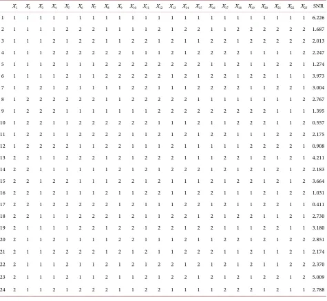
DOI: 10.4236/jss.2019.78012 169 Open Journal of Social Sciences In this step, 23 indexes are regarded as the features of multidimensional po-verty. We take each feature into two levels, that is level-1 means including the feature and level-2 means excluding the feature. We distribute the 23 features to the first 23 columns of an

( )

24 2

L array. For each run of the OA, The features with level-1 are used to construct an MS. And we calculate the MDs related to the 83 abnormal samples on the basis of the MS. The larger-the-better SNR is computed for each run by using (6) with the MDs of abnormal samples. The distribution of features in the OA and the SNR are shown in Table 2. After ac-quiring the SNR of each run, the effect gain of each index is computed and plot-ted into a graph, as shown in Figure 3. According to the value of gain, we keep the positive gain and removing the negative gain, as shown in Table 3.

The number of indexes of multidimensional poverty was reduced from 23 to 17, allocated by positive gains. Take the case of gain > 0, the preserved features are X4, X5, X6, X7, X8, X9, X10, X11, X14, X15, X17, X18, X20, X21, X22 and X23, the nor-mal group of 17 indexes is used to reconstruct a reduced model measurement scale. In the same way, we apply 83 abnormal samples to demonstrate the MS. Figure 4 depicts the MD allocations under the reduced model, it denotes that the new MS is good. After confirming the effectiveness of the reduced model measurement scale, a threshold is determined using (8) as follows:

1

TD 1 0.853 2.182

1 0.01 0.048

= + × ≈

+ −

Step 4: Future Diagnosis with Useful Features

For this reduced MS with 17 indexes, using 2.182 to be threshold leads to 90.244% accuracy of classification on the training set, which is shown in Figure 4. In the end, we use the test set to validate the classification performance of the reduced model. The MDs of the test set are calculated using (5), and the distri-bution of MDs are shown in Figure 5. For this reduced model with 14

DOI: 10.4236/jss.2019.78012 170 Open Journal of Social Sciences

Table 2.

( )

L OAs.

X1 X2 X3 X4 X5 X6 X7 X8 X9 X10 X11 X12 X13 X14 X15 X16 X17 X18 X19 X20 X21 X22 X23 SNR

1 1 1 1 1 1 1 1 1 1 1 1 1 1 1 1 1 1 1 1 1 1 1 1 6.226 2 1 1 1 1 2 2 2 1 1 1 1 2 1 2 2 1 1 2 2 2 2 2 2 1.687 3 1 1 1 2 1 2 2 1 1 2 2 1 2 1 1 2 2 1 2 2 2 2 2 2.013 4 1 1 1 2 2 2 2 2 2 1 1 1 2 1 2 2 2 2 1 1 1 1 2 2.247 5 1 1 1 2 1 1 1 2 2 2 2 2 2 2 2 1 1 2 1 1 2 2 1 1.274 6 1 1 1 1 2 1 1 2 2 2 2 2 1 2 1 2 2 1 2 2 1 1 1 3.973 7 1 2 2 1 2 1 1 1 1 2 2 1 1 1 2 2 2 2 1 1 2 2 1 3.004 8 1 2 2 2 2 2 2 1 1 2 2 2 2 2 1 1 1 1 1 1 1 1 2 2.767 9 1 2 2 2 1 1 1 1 1 1 1 2 2 2 2 2 2 2 2 2 1 1 1 1.395 10 1 2 2 1 1 2 2 2 2 2 2 1 1 1 2 1 1 2 2 2 1 1 2 0.557 11 1 2 2 1 1 2 2 2 2 1 1 2 1 2 1 2 2 1 1 1 2 2 2 2.175 12 1 2 2 2 2 1 1 2 2 1 1 1 2 1 1 1 1 1 2 2 2 2 1 0.908 13 2 2 1 1 2 2 2 1 2 1 2 2 2 1 1 1 2 2 1 2 1 2 1 4.211 14 2 2 1 1 1 1 1 1 2 1 2 1 2 2 2 1 2 1 2 1 2 1 2 2.183 15 2 2 1 2 2 1 1 1 2 2 1 2 1 1 1 2 1 2 2 1 2 1 2 3.664 16 2 2 1 2 1 1 1 2 1 1 2 2 1 1 2 2 1 1 1 2 1 2 2 1.031 17 2 2 1 2 2 2 2 2 1 2 1 1 1 2 2 1 2 1 1 2 2 1 1 0.411 18 2 2 1 1 1 2 2 2 1 2 1 1 2 2 1 2 1 2 2 1 1 2 1 2.730 19 2 1 1 1 1 2 2 1 2 2 1 2 2 1 2 2 1 1 1 2 2 1 1 3.180 20 2 1 1 2 1 1 1 1 2 2 1 1 1 2 1 1 2 2 1 2 1 2 2 2.851 21 2 1 1 2 2 2 2 1 2 1 2 1 1 2 2 2 1 1 2 1 1 2 1 2.174 22 2 1 1 1 2 1 1 2 1 2 1 2 2 1 2 1 2 1 2 1 1 2 2 2.370 23 2 1 1 1 2 1 1 2 1 1 2 1 2 2 1 2 1 2 1 2 2 1 2 5.009 24 2 1 1 2 1 2 2 2 1 1 2 2 1 1 1 1 2 2 2 1 2 1 1 2.788

Table 3. Indexes after reduced model.

X1 Per capita income of the household X14 Assisted living assets

X4 Accessibility of Public Education X15 Quantity of cultivated land

X5 Healthy conditions X17 Per capita housing area

X6 Sanitation facilities X18 Congestion

X7 Expenditure for health X20 Lighting conditions

X8 Accessibility of healthcare X21 Ventilate conditions

X9 Cooking water X22 Air condition

X10 Cooking fuel X23 Noisy conditions

DOI: 10.4236/jss.2019.78012 171 Open Journal of Social Sciences

Figure 4. The distribution of MDs of the rural households inspection training set (re-duced model with 17 features).

Figure 5. The distribution of MDs of the rural households inspection test set (reduced model with 17 features).

attributes, using 2.724 to be the threshold resulted in 90.503% classification ac-curacy on the training set. These results verified the effectiveness of the proposed method for the recognition of multidimensional poverty.

3.3. Discussion

DOI: 10.4236/jss.2019.78012 172 Open Journal of Social Sciences the poor population. The health conditions of the households were a barrier to the prevention of falling into “disease-poverty-disease” and breaking down in-tergenerational poverty caused by poor sanitation. At the same time, for families with housing problems, they need the transfer income to achieve poverty reduc-tion because of a low level of asset possession. Thus, we need to improve the liv-ing and health conditions of poor households to complete poverty alleviation.

4. Conclusions

This paper uses MTS to construct a model to recognize poverty from the multi-dimensional perspective. MTS can be used not only to realize the classification of rural households but also to identify the useful features from the system of multidimensional poverty. Besides, when using MTS in real performance, setting a threshold can distinguish between two types of samples and avoid overfitting problems. Finally, this study uses the MTS to recognize poverty with CLDS 2014 dataset. The case study aims to remove eliminate the redundant features and improve the accuracy of recognition. The results denote that the number of fea-tures is effectively reduced from 23 to 17 without losing accuracy. Therefore, Poverty recognition based on MTS is easy to apply and popularize in poverty al-leviation work.

This paper has three contributions. First, the concepts, principles and compu-tational process of MTS are described in detail. This helps us research this diag-nostic method. Second, a multidimensional poverty index system is constructed from six dimensions, which includes income, education, health, living, asset, and housing. Finally, we successfully introduced MTS to recognize multidimensional poverty. With the case study, this paper indicates that MTS in poverty reorgani-zation is robust and practicability and provides methodological support for po-verty recognition. In addition, healthy, cultivated land, income, and electricity are the main reason for the difference between the poor and non-poor in the case study. Therefore, we should enhance income and improve farming effi-ciency. For policy-making, improving rural living and health conditions by strengthening public services and infrastructure should also be concerned in the poverty alleviation.

However, there are some significant issues that need to be discussed in our future study. In the multidimensional poverty index system, the multicollineari-ty problem is unavoidable. That will lead to some errors in establishing the cor-relation matrix and influence the construction of MS. This is one of the signifi-cant research subjects that will be tackled in the near future.

Funding

DOI: 10.4236/jss.2019.78012 173 Open Journal of Social Sciences

Conflicts of Interest

The authors declare no conflicts of interest regarding the publication of this pa-per.

References

[1] Sen, A. (1976) Poverty: An Ordinal Approach to Measurement. Econometrica, 44,

219-231. https://doi.org/10.2307/1912718

[2] World Bank (2001) China: Overcoming Rural Poverty. World Bank, Washington

DC.

[3] Baulch, B. and Masset, E. (2003) Do Monetary and Nonmonetary Indicators Tell

the Same Story about Chronic Poverty? A Study of Vietnam in the 1990s. World

Development, 31, 441-453. https://doi.org/10.1016/S0305-750X(02)00215-2

[4] Laderchi, C.R., Saith, R. and Stewart, F. (2003) Does It Matter That We Do Not

Agree on the Definition of Poverty? A Comparison of Four Approaches. Oxford

Development Studies, 31, 243-274. https://doi.org/10.1080/1360081032000111698

[5] Bourguignon, F. and Chakravarty, S.R. (1998) The Measurement of

Multidimen-sional Poverty. DELTA Working Papers.

[6] Hagenaars, A. (2001) A Class of Poverty Indices. International Economic Review,

28, 583-607. https://doi.org/10.2307/2526568

[7] Lugo, A.M. (2011) Heterogeneous Peer Effects, Segregation and Academic

Attain-ment. Policy Research Working Paper.

[8] Tsui, K.Y. (2002) Multidimensional Poverty Indices. Social Choice & Welfare, 19, 69-93. https://doi.org/10.1007/s355-002-8326-3

[9] Bourguignon, F. and Chakravarty, S.R. (2003) The Measurement of

Multidimen-sional Poverty. The Journal of Economic Inequality, 1, 25-49. https://doi.org/10.1023/A:1023913831342

[10] Alkire, S. and Foster, J. (2011) Counting and Multidimensional Poverty

Measure-ment. Journal of Public Economics, 95, 476-487. https://doi.org/10.1016/j.jpubeco.2010.11.006

[11] Abu, M.Y., Nor, E.E.M. and Rahman, M.S.A. (2018) Costing Improvement of

Re-manufacturing Crankshaft by Integrating Mahalanobis-Taguchi System and Activi-ty-Based Costing. IOP Conference Series: Materials Science and Engineering, 342,

Article ID: 012006. https://doi.org/10.1088/1757-899X/342/1/012006

[12] Reyes-Carlos, Y.I., Mota-Gutiérrez, C.G. and Reséndiz-Flores, E.O. (2017) Optimal

Variable Screening in Automobile Motor-Head Machining Process Using

Metaheu-ristic Approaches in the Mahalanobis-Taguchi System. International Journal of

Advanced Manufacturing Technology, 95, 3589-3597. https://doi.org/10.1007/s00170-017-1348-0

[13] Chen, J., Cheng, L., Yu, H., et al. (2018) Rolling Bearing Fault Diagnosis and Health

Assessment Using EEMD and the Adjustment Mahalanobis-Taguchi System.

In-ternational Journal of Systems Science, 49, 147-159. https://doi.org/10.1080/00207721.2017.1397804

[14] Chang, Z.P., Cheng, L.S. and Liu, J.S. (2016) 2-Plus Choquet Integral Multi-Attribute

Decision Making Method Based on MTS. Journal of Management Engineering, 30,

133-139.

[15] Taguchi, G. and Jugulum, R. (2007) The Mahalanobis-Taguchi Strategy: A Pattern

DOI: 10.4236/jss.2019.78012 174 Open Journal of Social Sciences

[16] Su, C.-T. and Hsiao, Y.-H. (2007) An Evaluation of the Robustness of MTS for

Im-balanced Data. IEEE Transactions on Knowledge & Data Engineering, 19, 1321-1332. https://doi.org/10.1109/TKDE.2007.190623

[17] Stiglitz, J.E., Sen, A. and Fitoussi, J.P. (2014) The Measurement of Economic

Per-formance and Social Progress Revisited. Documents de Travail de l’OFCE, 19,

115-124.

[18] Sugden, R. (1986) Commodities and Capabilities. The Economic Journal, 96, 820-822.