Analysis of Thermal Behavior of High Frequency
Transformers Using Finite Element Method
Hossein Babaie, Hassan Feshki Farahani
Ashtian Branch, Islamic Azad University, Tehran, Iran. Email: {hbabaei2002, hfeshki}@yahoo.com
Received August 15th, 2010; revised September 17th, 2010; accepted September 20th, 2010.
ABSTRACT
High frequency transformer is used in many applications among the Switch Mode Power Supply (SMPS), high voltage pulse power and etc can be mentioned. Regarding that the core of these transformers is often the ferrite core; their functions partly depend on this core characteristic. One of the characteristics of the ferrite core is thermal behavior that should be paid attention to because it affects the transformer function and causes heat generation. In this paper, a typical high frequency transformer with ferrite core is designed and simulated in ANSYS software. Temperature rise due to winding current (Joule-heat) is considered as heat generation source for thermal behavior analysis of the trans-former. In this simulation, the temperature rise and heat distribution are studied and the effects of parameters such as flux density, winding loss value, using a fan to cool the winding and core and thermal conductivity are investigated.
Keywords: High Frequency Transformers, Thermal Behavior, Ferrite Core and Finite Element Analysis
1. Introduction
Magnetic components design plays a key role in achiev-ing high efficiency, low volume and reasonable price of power electronic equipment. With the advent of higher switching frequencies and power densities in power elec-tronic circuits, it is important to ensure that magnetic components, such as transformers and inductors, operate within the limits defined by the thermal specifications of the circuit. Temperature rise depends on the power losses through the laws of the heat transfer theory. In order to obtain an accurate value of the maximum temperature of the device during the design process, it is necessary to apply an accurate thermal model. It is necessary of a trade-off between thermal distribution accuracy (direc-tions through heat transfer is considered, constant ther-mal properties, feedback with the magnetic model, steady state models, etc) and the complexity of the ther-mal model that is obtained.
Losses in the magnetic components are important design parameters. In many high-frequency designs, magnets are limited by their losses. Thus, it is extremely important for the designer to have a good practical model for estimating the losses under various excitations that are frequently en-countered in power electronics design. There are two major components of the losses [1-9] in a magnetic component: the core loss (i.e., the losses in the magnetic material which is used as core) and the winding losses. High-frequency
conductor losses for power electronics applications have been considered by a number of authors [8,9]. There are models provided by different manufacturers [10-12], that are synthesized in a simple expression for the calculation of the temperature rise. They provide the average temperature in the outer surface of the device.
Most of thermal models for magnetic components are analytical and assume 1D heat transfer [13-15]. These models are based on thermal networks and commonly consider only steady state, constant thermal properties, concentrated and uniform power losses and no thermal feedback with the electric properties. However, the ther-mal distribution is 2D/3D for most of cases, even if the magnetic field exhibits a 1D distribution.
The thermal design is usually somewhat neglected as it is often not clear which theory and coefficients should be used and experiments are time consuming. In this article, by designing a typical high-frequency trans-former with ferrite core, its thermal behavior is investi-gated. Many parameters such as flux density, winding loss value, using a fan to cool the winding and core and thermal conductivity have effects on the ferrite tempera-ture which is simulated with ANSYS software.
2. Calculating the Heat Generation Caused
by Winding and Investigating Its
Effective Parameters
generate heat by passing the current and this heat is transmitted to other parts. For a winding with resistance Rj, the power loss can be written as:
2 , cu j j j
P I R (1)
Which the jth winding resistance is as follow:
, j j w j l R A
(2)
Where:
j jl n MLT
(3),
A u j w j j W K A n
(4)
In Equation (3), MLT is mean length per turn (cm). By considering Equation (2) to Equation (4), the power loss of jth winding is as follow:
2 2, j j cu j
A u j
n i MLT
P
W K
(5)
And the total power dissipation is the sum of the power losses for each winding:
2 2 , 1 k j j cu tot jA u j
n I MLT P W K
(6)The loss in winding is optimal providing that [16]:
,
1 k
cu tot j j
j A u MLT P W K
n I
(7) [image:2.595.317.533.89.184.2]According to Equation (7), it can be found out that the power loss or generated heat depends on parameters such as ρ (wire effective resistivity), Ku (winding fill factor), turns, winding current and MLT (mean length per turn). So, these are effective parameters on generation heat source. In a transformer, if the primary voltage is like Figure 1, then the following equations will be written:
21
1 1
t
t v t dt
(8)1
max 1
1 m
2 c 2 c
B n
n A B A
1
ax
(9)
By substituting Equation (9) in Equation (7), the result can be written as:
2 2 2
2 1
1 2 2
1
tot tot
cu
A u u A c max
A B C
MLT I I MLT
P n
W K k W A B
(10) where: 1 1 k j tot j j n I I n
Area λ1
t1 t2
Vg
-Vg
0 0
v1(t)
Figure 1. Transformer primary voltage.
Equation A i
lectrical ore and
(10) consists of three parts in which part characteristics and B and C include c
s e
magnetic characteristics respectively.
The core loss is obtained from the following equation:
fe fe max c m
P k B A l (12) Kfe
frequencies. Ac is core cross-section agnet
and its effec-tiv rmer for full bridge con-is core loss coefficient which con-is different for various
al area and lm is m ic path length. The typical value of β for ferrite core is 2.6 < β < 2.8. Kfe is drastically increased by in-creasing the frequency. In addition, Kfe depends on core temperature and Bmax. The dependency of Kfe on fre-quency, Bmax and temperature can be obtained from core characteristics. In choosing the core when combined with different alloys, there has been always trade-off between saturated magnetic flux density and the core loss. Using materials with high Bsat leads to volume, size and price reduction. But these materials cause more core loss.
3. Transformer Characteristic for
Full-Bridge Converter
To study the temperature rise in ferrite core e parameters, a sample transfo
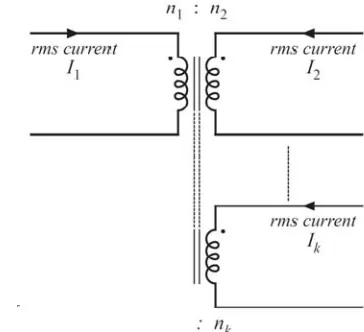
[image:2.595.325.507.523.689.2]verter with two secondary windings and one primary winding is chosen which can be seen in Figure 2 [16].
Figure 2. Transformer for full bridge converter with two outputs and one input.
Table 1. Parameters of designed transformer for full bridge converter
75kHz Transformer frequency
110 :5 :15 ratio
Turn
0.75 Duty cycle
EE40
β
Selected core
/T cm3
4×10 Ω-cm -µsec
x
0 mW 7.6 W kfe
2.6
β
0.25
-6
Ku
1.72
ρ
800 V
λ1
5.7 A I1
66.1 A I2
9.9A I3
14.4 A Itot
80 mT Bma
22 n1
1 n2
3 n3
23 Pfe
3.89 W Pcu
4.12 W Ptot
The ined parameters for th mer are listed in ble 1. The core and winding losses calculated for tra
indings is Figure 3.
in Table 2.
that the heat transfer be-the transformer has been
obta is transfor
Ta
nsformer are equal to 230 mW and 3.89 W respectively. These losses can be used as heat generating source in modeling and simulating the transformer in ANSYS.
4. Transformer Modeling in ANSYS
In this part, transformer with two secondary w modeled in ANSYS software which is shown in
The distance between each winding is 0.5 mm. the pri-mary winding is 20 mm long and 2 mm wide which this cross-sectional area includes 22 turns primary winding. This area for secondary winding is 20 mm2 (1 mm × 20 mm) which is for one turn. Also, another secondary winding is 20mm long and 0.5mm wide which consists of three turns.
The electrical and thermal characteristics for different parts of transformer are listed
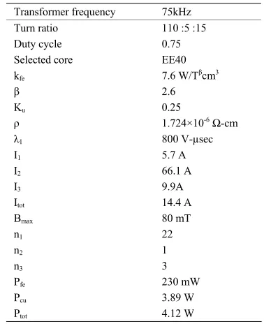
5. Simulation Results
In this simulation, it is assumed tween winding and core of
naturally done (natural convection). So, the film coeffi-cient varies from 10 W/m2·ºC to 25 W/m2·ºC when there is natural convection. The film coefficient is considered equal to 10 W/m2·ºC. The total cross-section of area is 70 mm2 and the power dissipation in this area is 3.89W. Therefore, the value of watt per square meter of area is equal to 55570 W/m2 which is used for heat generation source in ANSYS. In Figure 4, temperature distribution
Core Winding
Air Air
[image:3.595.76.265.113.345.2]Figure 3. Modeled transformer in ANSYS.
Table.2 ifferent
arts of transformer
Electrical and thermal characteristics for d p
Material Parameter
Air Ferrite Core
Copper
1.09 8900
Density, ρ [kg/m3] 8900
1006 750
387
Specif kgºC]
T ,
ic heat, c [J/
0.027 0.004
385 hermal conductivity
λ [W/(m·K)]
Figure 4. Thermal distribution in transformer.
throug ottest
oint is primary winding and middle leg of ferrite core h the transformer is shown. In this figure, the h p
[image:3.595.308.539.331.591.2]Figure 5. Thermal distribution in core.
Therma and it is
m ized in primary winding corners which are about 42
ity variation on tem-has been investigated.
. In l flux in this case is shown in Figure 6
axim
8.69 W/m2. Regarding this matter and according to Figure 4, it can be pointed out that the corners tempera-tures are lower than that in other parts.
5.1. Variation of Flux Density
In this part, the effect of flux dens perature distribution in transformer
For this purpose, the flux density is decreased from 80 mT to 120 mT. According to Equation (10), the power loss is in inverse proportion with the square of flux density and by this change, the power loss is decreased 2.25 times.
The heat distribution for this condition is shown in Figure 7 in which the hottest point is about 55.309ºC
Figure 7. Thermal distribution in transformer (Decreasin
is case, one of the secondary windings temperatures
sed in
gure 4 with Figure 8, we can make th
2·ºC to 120
the fan, almost all windings have the same te
g a Fan to Cool the Core
cooled by a fan
to this figure, the core ambient temperature is almost
g flux density).
th
(neighbor of primary winding) is approximately equal to primary winding temperature (the highest temperature).
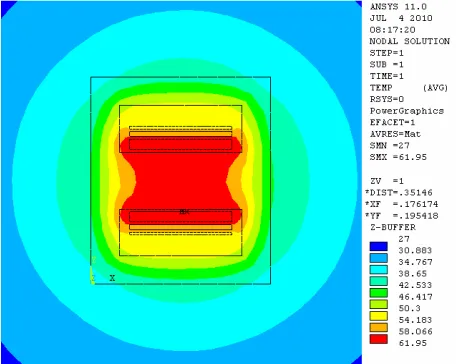
5.2. Variation of the Ambient Temperature
In this case, it is supposed that the transformer is u 40ºC temperature. So, it is observed that the maximum temperature inside the transformer has been slightly in-creased and has reached to 61.971ºC. In this case, the maximum temperature is in primary winding and core middle leg as well.
By comparing Fi
e conclusion that regarding the proximity of core sides to heat source and warmer environment, the sides’ tem-perature are higher than that in up and down of core.
5.3. Using a Fan to Cool the Winding
The film coefficient varies from 50 W/m
W/m2·ºC when there is forced convection. For this case the film coefficient has been changed from 10 W/m2·ºC to 50 W/m2·ºC. The temperature distribution is shown in Figure 9.
By using
mperature of 52.508ºC. By comparing this figure with Figure 4, it can be understood that using the fan leads to winding temperature reduction from 61.962ºC to 52.508ºC. By this analysis, the appropriate fan can be chosen.
5.4. Usin
In this case, it is supposed that core is
(the film coefficient is 50 W/m2.ºC). The heat distribu-tion in this condidistribu-tion is plotted in Figure 10. According
Figure 8. Thermal distribution in transformer (Increas ng the ambient temperature).
i
Figure 9. Thermal distribution in transformer (Using fan to cool the winding).
shows that changing the film coeffi-ient causes suitable increase in core temperature
nductivity W/(m.K).
ffect (61.95ºC) on the temperature but the ther-m
ermal behavior of different cores has his purpose, first for a typical trans- equal. This figure
c
(61.95ºC).
5.5. Variation of Thermal Conductivity
On of the other studied parameters is thermal co that it is changed from 0.004 W/(m·K) to 0.008
Thermal distribution for this mode is shown in Figure 11.
This figure shows that the thermal conductivity has a little e
aldistribution around the transformer is uniform as a circle from centre of transformer.
6. Conclusions
[image:5.595.57.272.85.258.2]In this paper, the th been studied. For t
Figure 10. Thermal distribution in transformer (Using fan to cool the core).
Figure 11. Thermal distribution in transformer (Increasing thermal conductivity).
heat is computed then it is totally imulated in ANSYS software. In this simulation, the
s-fo
former, the generation s
thermal analysis and heat distribution were studied. Then, the effects of parameters such as flux density, winding loss value, the film coefficient have been investigated.
According to obtained results, in case of using a fan to cool the winding, the maximum temperature of tran
[image:5.595.57.273.299.475.2] [image:5.595.308.536.303.485.2]REFERENCES
[1] S. N. Talukda steresis Models for
System Studie n Power Appa
, pp.
gic,” McGraw-Hill, New York, 1969.
rromagnetic
Materi-h Diagrams,” IEEE Transaction
EE
Wire effective resistivity (Ω-cm)
I Total rms winding current, ref to primary (A) /n1, n3/n1, etc
ion (W)
t (W/cm3Tβ)
area (cm2
) core corners have the lower temperature in comparison with other parts. This part has the maximum thermal flux as well.
r and J. R. Bailey, “Hy
s,” IEEE Transactions o
[9]
ratus [10] Power Conversion and Line Filter Applications.
and Systems, Vol. 95, No. 4, 1976, pp. 1429-1434.
[2] C. C. Wong, “A Dynamic Hysteresis Model,” IEEE
Transactions on Magnetics, Vol. 24, No. 2, 1988
1966-1968.
[3] D. R. Bennion, H. D. Crane and D. Nitzan, “Digital Magnetic Lo
[4] F. Presiach, “On the Magnetic Aftereffect,” Zeitschrift für
Physik, Vol. 94, 1935, pp. 227-302.
[5] R. D. Vecchio, “An Efficient Procedure for Modeling Complex Hysteresis Processes in Fe
als,” IEEE Transactions on Magnetics, Vol. 16, No. 5, 1980, pp. 809-811.
[6] D. L. Atherton, B. Szpunar and J. A. Szpunar, “A New
Approach to Presiac on [1
Magnetics, vol. 23, No. 3, May 1987, pp. 1856-1865.
[7] B. Szpunar, D. Atherton and M. Schonbachler, “An Ex-tended Presiach Model for Hysteresis Processes,” IE
Transactions on Magnetics, Vol. 23, No. 5, 1987, pp.
3199-3201.
Nomenclature
[8] J. P. Vandelac and P. D. Ziogas, “A Novel Approach for Minimizing High Frequency Transformer Copper Losses,” IEEE Transaction on Power Electronics, Vol. 3, No. 2, 1988, pp. 266-277.
B. Carsten. “High Frequency Conductor Losses in Switched Mode Magnetic,” in Proc. HFPC Con$ Ventura, CA: Intertec Communications Inc., May 1986.
[11] Design of low profile high frequency transformers-A new tool in SMPS design-. Philips Magnetic Products. Appli-cation note. May.1990.
[12] Kool Mu Powder Cores Data Book. Magnetics.
[13] L. M. Escribano, R. Prieto, J. A. Cobos and J. Uceda, Thermal Modeling of Magnetic Components: A Survey,”
Proceeding of 28th Annual Industrial Electronics Society
Conference of the IEEE, Sevilla, 5-8 November 2002, pp.
1336-1341.
[14] L. M. Escribano, R. Prieto, J. A. Oliver, J. A. Cobos and J. Uceda, “Analytical Thermal Model for Magnetic Com-ponents,” Proceedings of 34th AnnualPower Electronics
Specialist Conference of the IEEE, 2003, pp. 861-866.
5] J. C. S. Fagundes, A. J. Batista and P. Viarouge, “Thermal Modeling of Pot Core Magnetic Components Used in High Frequency Static Converters,” IEEE Transactions on
Magnetic, Vol. 33, No. 2, March 1997, pp. 1710-1713.
[16] R. W. Ericksonand D. Maksimo, “Fundamentals of Power Electronics,” 2nd Edition, Springer, Berlin, 2002.
ρ tot
n2 Desired turns ratios (V-sec) λ1
P
Applied primary volt-sec tot
K
Allowed total power dissipat u
β
Winding fill factor Core loss exponent Kfe
A
Core loss coefficien c
W
Core cross-sectional ) Core window area (cm2) A
MLT l
Mean length per turn (cm) e
A 1, …
Magnetic path length (cm
w ΔB