Predicting the Corona for the 21 August 2017 Total
Solar Eclipse
Zoran Miki ´c1,*, Cooper Downs1, Jon A. Linker1, Ronald M. Caplan1, Duncan H. Mackay2, Lisa A. Upton3, Pete Riley1, Roberto Lionello1, Tibor T ¨or ¨ok1, Viacheslav S. Titov1,
Janvier Wijaya1, Miloslav Druckm ¨uller4, Jay M. Pasachoff5,6, and Wendy Carlos7
1Predictive Science, Inc., San Diego, CA 92121, USA
2School of Mathematics and Statistics, University of St Andrews, St Andrews, Fife, KY16 9SS, UK
3High Altitude Observatory, National Center for Atmospheric Research, Boulder, CO 80301, USA
4Institute of Mathematics, Faculty of Mechanical Engineering, Brno University of Technology, Czech Republic
5Williams College–Hopkins Observatory, Williamstown, MA 01267, USA
6Carnegie Observatories, Pasadena, CA 91101, USA
7New York City, NY 10003, USA
The total solar eclipse that occurred on 21 August 2017 across the United States provided an op-portunity to test a magnetohydrodynamic model of the solar corona driven by measured magnetic fields. For the first time we used a new heating model based on the dissipation of Alfv´en waves, and a new energization mechanism to twist the magnetic field in filament channels. We predicted what the corona would look like, one week before the eclipse. Here we describe how this predic-tion was accomplished, and we show that it compared favorably with observapredic-tions of the eclipse in white light and extreme ultraviolet. The model allows us to understand the relationship of observed features, including streamers, coronal holes, prominences, polar plumes, and thin rays, to the magnetic field. We show that the discrepancies between the model and observations arise from limitations in our ability to observe the Sun’s magnetic field. Predictions of this kind provide opportunities to improve the models, forging the path to improved space weather prediction.
Background
Eclipses have long been a source of wonder and fascination, but they also have a unique place in the scientific discovery process. On 21 August 2017, a celestial spectacle delighted millions of people across the United States, as a total solar eclipse swept across the country. It provided an opportunity to test our understanding of the physics of the solar corona1–3, the region of the Sun’s atmosphere where the gas is heated to over a million degrees by processes that are still not fully understood4–6. During totality a solar eclipse reveals the faint corona that is normally hidden from view, exposing intricate structures that are shaped by the magnetic field, including streamers, polar plumes, rays, and prominences. The coronal magnetic field is the source of the energy that is released during the solar flares7 and coronal mass ejections that can damage Earth-orbiting satellites and cause power outages. It dominates the structure and dynamics of the corona, but is difficult to observe above the photosphere and chromosphere. It is of intense scientific interest to understand how the magnetic field emerges from beneath the Sun’s surface, how it evolves, when it is about to erupt, and how such ejections travel through interplanetary space. These eruptions have the potential to trigger a geomagnetic storm when they interact with the Earth’s magnetic field.
ob-servations of the Sun’s magnetic field in the photosphere to the coronal structures that are unveiled during an eclipse. Complementary measurements of extreme ultraviolet (EUV) and X-ray emission from space offer an additional perspective. White-light observations of the corona are made routinely from ground-based observatories and spaceborne coronagraphs, but neither can image the lowest layers of the corona, or capture the finest details that are observed during eclipses (though future space coronagraphs promise to narrow this gap8). Consequently, even with today’s detailed space measurements of the Sun, eclipses play a unique role in this discovery process9–11, especially since the expense of the instrumentation re-quired is relatively modest.
It has been said that prediction is the ultimate test of a scientific theory. It was during the 1919 eclipse that Eddington and colleagues verified Einstein’s theory of general relativity to great acclaim, confirming a prediction for the shift in the apparent position of stars by warping of space by the Sun12 (though the accuracy of the measurement is not without controversy13–15). Our group has made routine predictions of the eclipse corona for over two decades16–18, during which time our models have improved steadily as a result of dramatic advances in computing power, but also through enhancements in the physics of the models. These improvements were driven in part by comparisons with eclipse predictions. In the future, these and similar models are expected to improve the forecasting of solar storms. In this article, we describe a prediction of the solar corona using a computer model that tests recent advances in theory and modeling with modern observations. The model employs two key innovations: a physics-based formulation that describes the heating of the corona over a broad range of conditions, and a novel approach for energizing the coronal magnetic field on global scales. A related prediction of this eclipse with a different model has also been made19, and is discussed below.
Predicting the Eclipse Corona
We predicted the structure of the corona one week prior to the eclipse, using a 3D magnetohydrodynamic (MHD) model to compute the interaction of the solar wind with the Sun’s magnetic field (see Methods). It tracks the exchange of energy between coronal heating, radiative losses, and thermal conduction along the magnetic field, and is fed by measurements of the magnetic field in the photosphere20–22. We used spaceborne measurements of the photospheric magnetic field from the Helioseismic and Magnetic Imager (HMI)23 aboard the Solar Dynamic Observatory (SDO)24, and a wave-turbulence-driven (WTD) model to heat the corona via low-frequency Alfv´en waves launched in the chromosphere25–27. A fraction of the outward-directed waves interact with reflected waves28 and dissipate, heating the corona.
Eclipses reveal the lowest regions of the solar corona, where prominences are often seen, embedded at the base of coronal streamers and pseudostreamers29. Several prominences were observed during the 21 August 2017 eclipse, as is typical during this declining phase of the solar cycle. These dense, cold structures are believed to be supported by magnetic fields in filament channels30–32. When a prominence is present within a streamer, it tends to produce an “inflated” appearance because of the extra magnetic pressure from the magnetic field (see Supplementary Figure 6). To model these features, we imple-mented a technique to introduce highly sheared magnetic fields in these channels, at locations that were determined by examining animated images of EUV emission observed by the Atmospheric Imaging As-sembly (AIA)33 on SDO (see Supplementary Figure5). This process increased the free magnetic energy, “energizing” the corona, as described in the Methods section.
synoptic chart is shown in Supplementary Figure2.) The parameters for the model, including the driving Alfv´en wave amplitude, were selected based on runs made during the previous two months (as discussed in the Methods section, and summarized in Supplementary Figure1). The calculation was begun on 11 August 2017, starting from one of these previous solutions. The corona was relaxed towards equilibrium by advancing the model for 60 hours of solar time in a dedicated queue at NASA’s Advanced Supercom-puting Center. At the final stage of our calculation, we introduced magnetic shear in filament channels, relaxing the corona for another 8 hours. These runs took a total of 54 hours of real time to advance 68 hours of solar time.
Since the corona responds to changes in the photospheric magnetic field, the accuracy of a prediction deteriorates over time. We would expect better accuracy during this declining phase of the solar cycle, when the Sun’s magnetic field changes more slowly than at solar maximum, and this was indeed the case. Flux transport models have promise in improving the accuracy of the evolving photospheric magnetic field. Indeed, the Surface Flux Transport (SFT) model has been used in conjunction with a potential field source-surface (PFSS) model to predict the structure of the coronal magnetic field for this eclipse19. While this simpler model does not predict coronal density and temperature, and does not produce non-potential coronal magnetic fields, it can be carried out rapidly. The flux transport model that we used to identify energized filament channels (see the Methods section) employs a magnetofrictional model in the corona, and produces nonpotential coronal fields34.
After completing the calculation, we synthesized observables that can be compared directly with observations taken during the eclipse. From the predicted electron density we computed the total and polarized brightness in white light35, quantities that are principally measured during eclipses. Polarized brightness can be useful in separating the significantly polarized K-corona, of solar origin, from the largely unpolarized fainter outer F-corona, whose main contribution is from interplanetary dust36. Using the distribution of temperature, we computed the EUV emission expected in various channels of the AIA telescope, as well as soft X-ray emission18,22,37. We also visualized the squashing factor38 Qthat emphasizes the fine spatial scales in the magnetic field, as discussed in the Methods section.
Comparison with Eclipse Observations
Our prediction was tested against photographs of the eclipse and spaceborne observations. Overall, the model predicted the general appearance of the corona, though many details were different. The princi-pal large-scale streamers that visually dominate the eclipse corona were predicted accurately. Figure1
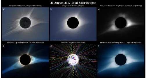
shows a comparison between two eclipse images and several predicted quantities from the MHD simula-tion. A series of photographs taken at different exposures by the Solar Wind Sherpas eclipse expedition in Mitchell, Oregon, were combined digitally and enhanced39 to emphasize the finest details in the corona (Fig. 1a). A different series of 14 photographs taken in Salem, Oregon, by the Williams College expedi-tion, were assembled digitally (Fig.1b) as described in the Methods section. It is difficult to produce a simulated image of what the eye sees during an eclipse, because of the accommodation of the eye to the wide range of brightness in the corona, but in our personal experience, it is likely to between Fig.1a and Fig.1b.
21 August 2017 Total Solar Eclipse
a
© 2017 Miloslav Druckmüller, Peter Aniol, Shadia Habbal
Image from Mitchell, Oregon (Sharpened)
© 2017 Wendy Carlos and Jay Pasachoff. All rights reserved.
b
Image from Salem, Oregon Predicted Polarized Brightness (Newkirk Vignetting) c
Predicted Magnetic Field Lines e
Predicted Squashing Factor (Volume Rendered) d
[image:4.612.54.557.64.335.2]Predicted Polarized Brightness (Log Unsharp Mask) f
Figure 1. Comparison between the observed and predicted eclipse corona. The images are oriented with terrestrial north up; solar north is 18.2◦counterclockwise from the vertical.
For an animation of pB at different longitudes see Supplementary Video 1. An alternate depiction of the coronal structure is obtained by using an “unsharp mask” on pB and displaying the result using a logarithmic scaling (Fig.1f).
Polar plumes, which are visible in the polar regions (Fig.1a), are seen to align with the magnetic field lines (Fig.1e), as shown inSupplementary Video 2, an animation that fades between the two images. The fine-scale features in the white-light corona (Fig.1a) are believed to be manifestations of the complexity of the underlying magnetic field. Although our calculations do not yet have enough resolution to resolve these spatial scales directly in the white-light corona, the magnetic field, as visualized byQ, does display similar fine-scale features (Fig.1d). Many of the variegated, high-Qstructures arise from the divergence of coronal field mappings as they approach the small-scale flux concentrations present in the photosphere. For an animation ofQat different longitudes seeSupplementary Video 3. Animations that fade between an eclipse image andQand pB are shown inSupplementary Video 4 andSupplementary Video 5. The complexity that is evident in the coronal magnetic field, and its associated topological consequences, including the presence of separatrices and quasi-separatrix layers (QSLs), has been termed the “separatrix web,” or S-web41–43. It may provide the key to the origin of the slow solar wind, which has a distinctly different structure and composition from the fast wind. A key development of our model is to capture, self-consistently, the propagation of Alfv´en waves, and the resultant coronal heating, in the backdrop of this magnetic complexity.
In addition to this comparison with eclipse observations, we compare with observations on other days to highlight interesting structures that are present in a three-dimensional model of the corona. In Figure2
EUV Emission on July 25, 2017
07/25/2017 11:50UT
b
AIA 193Å Emission
07/25/2017 11:50UT
c
AIA 211Å Emission AIA 171Å Emission
07/25/2017 11:50UT
a
d
Synthesized 171Å Emission
Log10DN/s
2
1 3 4
e
Synthesized 193Å Emission
2
1 3 4
Log10DN/s
f
Synthesized 211Å Emission
2
1 3 4
[image:5.612.132.482.65.344.2]Log10DN/s
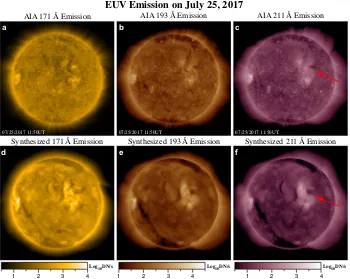
Figure 2. Comparison between observed and predicted EUV emission.Observed EUV emission (a,
b, andc) in the 171 ˚A (FeIX), 193 ˚A (FeXIIandXXIV), and 211 ˚A (FeXIV) AIA channels, deconvolved with the point-spread function, on 25 July 2017, one solar rotation prior to the eclipse, compared with simulated emission (d,e, andf) from the prediction. The images are oriented with solar north up. The red arrows indicate the diffused active region with a nonpotential character.
of observed emission across a wide variety of solar features, including coronal holes, which appear as extended dark regions, and active regions, which appear bright. There also are significant differences in the details, associated with temporal changes of the corona and the limited spatial resolution of the model, so the agreement must be considered qualitative. Coronal holes are locations with largely unipolar magnetic field in the photosphere, in which the magnetic field lines are open, and are believed to be the source of the fast solar wind. At this phase of the solar cycle the polar coronal holes are ubiquitous, and sometimes extend to lower latitudes. Since the level of emission is sensitive to the amount and distribution of coronal heating, this confirms that the WTD model performs well. The diffused active region at latitude 22◦N, longitude 305◦, indicated by red arrows in Figure2, shows a significant nonpotential character, a consequence of the magnetic shear introduced along the polarity inversion line (PIL) passing through it (see Supplementary Figure5).
Unraveling the Sun’s Complexity
b
Q (including all features)
c
Q (removing masked volume)
a
Eclipse Image
Field Lines, Br, & Open-Field Regions
2 3 4
1
e d
[image:6.612.130.483.63.428.2]Volume-Rendered Q & Mask
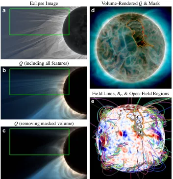
Figure 3. Investigating the origin of equatorial rays.The equatorial rays seen in the eclipse imagea
are present in the volume-renderedQimageb(within the green box). c, When the structures that connect to the low-latitude portion of the coronal hole are removed (within the volume that maps to the interior of the mask outlined in orange indande), the rays disappear, verifying that their source is within the coronal hole. d, A view ofQwhen the Sun is rotated by 117◦about its axis to make the coronal hole visible. The red arrows point to the bases of 4 prominent rays. e, Open-field regions (transparent gray),Br with blue (red) indicating negative (positive) values, and traces of magnetic field
lines in arbitrary colors. The numbers 1–4 inemark the parasitic polarity at the base of the rays. It is also evident fromdandethat the polar plumes in the northern coronal hole emanate from locations with parasitic polarity.
rays are indeed similar to plumes45, since they connect at their base to locations in coronal holes with parasitic magnetic polarity (Fig.3e). Even though the simulated rays qualitatively resemble the observed ones, their individual brightness and locations are different. These are likely to be transient features be-cause they are associated with small regions of parasitic polarity that cannot be captured using synoptic data.
Filaments, Prominences, and Coronal Holes on August 1, 2017
Field Lines, Br, & Open-Field Regions
c
PS
P
P P
CH
FR AR
Volume-Rendered Q
d
PS
P
P P
CoMP 1074 nm Enhanced Intensity
b
PS
P
P P
AR
08/01/2017 18:02UT
AIA Sharpened 193Å Emission
a
PS FC
P
P P
CH
AR
[image:7.612.130.484.145.533.2]08/01/2017 18:02UT
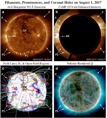
Figure 4. Comparison between observed features and model predictions. a, Sharpened AIA 193 ˚A EUV emission on 1 August 2017. b, Enhanced intensity of the 1074 nm FeXIIIcoronal emission line from the MLSO CoMP instrument.c, Model predictions, including open-field regions (transparent gray),Br with blue (red) indicating negative (positive) values, and traces of magnetic field lines in
arbitrary colors.d, Volume-rendered squashing factorQ. Bright loops in an active region (AR) are visible on the limb (aandb). Dark coronal holes (CH) in EUV emissionacorrespond with open-field regions in the modelc. Dark filament channels (FC) in emissionacorrespond with the location of a twisted flux rope (FR) in the modelc. Cavities associated with prominences (P) and a pseudostreamer (PS) on the limbs in AIA and CoMP,aandb, agree with magnetic structures in the model,candd.
locations are the sites of filaments, in which the coronal plasma condenses to chromospheric temperatures, which appear in Hα and in the 304 ˚A AIA channel. We illustrate these features in Figure 4, in which we compare observations with predictions on 1 August 2017. Figure 4a shows a 193 ˚A AIA image, sharpened46 to emphasize fine details. The northern coronal hole (marked CH), which appears dark, can be seen to extend to equatorial latitudes. This area corresponds to locations with open field lines in the model (Fig.4c), in a positive-polarity region (red), with small parasitic negative-polarity intrusions (blue). The twisted magnetic fields in a long flux rope (marked FR in Fig. 4c), correspond to a dark filament channel with the same shape in the EUV image (marked FC in Fig.4a). Supplementary Video 9
compares the locations of energized filament channels with a synoptic map of AIA 193 ˚A emission. On the limbs, prominences are associated with coronal cavities47. These are locations with reduced EUV emission that coincide with the flux ropes that magnetically support the cold and dense material in prominences. The 193 ˚A emission from AIA (Fig.4a) and the enhanced intensity from the 1074 nm FeXIIIcoronal emission line measured at Mauna Loa Solar Observatory (MLSO) with the CoMP instru-ment48 (Fig.4b) show the cavities associated with the flux ropes/prominences. A volume rendering ofQ (Fig. 4d), which emphasizes the shape of magnetic structures on the limbs, shows good correspondence between the twisted flux ropes in the model that extend to the solar limbs and the cavities associated with prominences (marked P) in these images. In particular, a pseudostreamer29 (marked PS), with two prominence cavities embedded in it, is clearly visible in AIA and CoMP on the southeast limb. The model shows the flux ropes that support these prominences in the same location (Fig.4c), and these are clearly visible in Q (Fig. 4d). Animations of Q (Supplementary Video 6) and the magnetic field lines (Supplementary Video 7) versus longitude aid in following the 3D structure of these flux ropes.
The Missing NW Pseudostreamer
One notable disagreement between our prediction and the observed corona is the small pseudostreamer29 that extends to large radius on the northwest limb (top center-right in Figs.1a and1b). The eclipse images show that it contains two prominences at its base, typical of pseudostreamers, which are associated with a double reversal (a “switchback”) in the large-scale polarity inversion line (PIL)29. This structure is not seen in the predicted pB images (Figs. 1c and1f), though the Qimage (Fig.1d) does show a tendency for an extended radial feature there. Careful analysis of the photospheric magnetic field synoptic chart used for the prediction (Supplementary Fig.2) shows that the requisite PIL switchback is not present near the northwest limb (latitude 50◦N, longitude 21◦), precluding the formation of a pseudostreamer there. The magnetic field measurements in that neighborhood date from 16–20 July 2017, so they are over a month old by eclipse time. Newer observations, from 12–16 August 2017, show that the magnetic fields in that location are evolving, and the switchback now extends to the northwest limb (see Supplementary Figure3), supporting the formation of a pseudostreamer. Interestingly, the SFT model correctly predicted a reversal at that location, as well as the associated pseudostreamer19.
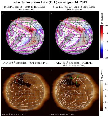
In Figure5we examine the PIL from different models at 21:52UT on August 14, 2017. This view is convenient to investigate the NW pseudostreamer because structures that were located at the west limb at eclipse time are at central meridian in this view. Fig. 5a shows photosphericBr and the PIL (black
the NW pseudostreamer was absent in our prediction. Fig. 5b makes the same comparison, but now with updated HMI magnetic field data (July 20–August 16) corresponding to CR2193 (Supplementary Figure3). The negative polarity (blue values) now reaches central meridian, implying that a prediction with this data would produce the NW pseudostreamer, an idea we intend to explore.
2.0 1.5 3.0 3.5 2.5 Log 10 D N /s 30 15 0 -15 -30 Br [G aus s]
Polarity Inversion Line (PIL) on August 14, 2017
-60 -40 -20 0 20 40 60 310 330
350 10 30 50 70 90
Br & PIL (Jul 20 – Aug 16 HMI Data)
+ SFT Model PIL b -60 -40 -20 0 20 40 60 310 330
350 10 30 50 70 90
AIA 193 Å: 08/14/2017 22:02UT
d
AIA 193Å Emission + HMI PIL
(Jul 20 – Aug 16 Data)
-60 -40 -20 0 20 40 60 310 330
350 10 30 50 70 90
Br & PIL (Jul 16 – Aug 11 HMI Data)
+ SFT Model PIL a -60 -40 -20 0 20 40 60 310 330
350 10 30 50 70 90
AIA 193 Å: 08/14/2017 22:02UT
c
AIA 193Å Emission + SFT Model PIL
Figure 5. Polarity Inversion Line Comparison. a,Br and the PIL (black line) from HMI data used for
the prediction, compared with the PIL from the SFT model (magneta line). Positive (negative)Brvalues
from HMI are shown in red (blue). Positive-polarity regions in the SFT model are shaded a transparent gray. b, Same asa, but with updated HMI data (July 20–August 16). c, An overlay of the SFT model PIL (white line) on an AIA 193 ˚A EUV emission image. The extended dark region indicates a coronal hole. d, An overlay of the PIL from the updated HMI data on the same 193 ˚A image. In these views, the NW pseudostreamer that was on the west limb at eclipse time is at central meridian. The red arrows show the switchback in the SFT model PIL that allows the NW pseudostreamer to form; the green arrows show the switchback in the PIL from HMI synoptic data. These PILs are discussed in the text.
[image:9.612.129.484.138.519.2]the negative-polarity region (red arrows) encroaches into the positive-polarity coronal hole, leading to an inconsistency. On the other hand, the PIL from the updated HMI data (Fig.5d) correctly stops short of the coronal hole boundary (green arrows).
Clearly, getting the most accurate representation of the magnetic field is of paramount importance when making predictions. As we have seen, synoptic magnetic field data, which are built up from ob-servations from a single vantage point over a solar rotation, can lead to inaccuracies. An alternative is to use a flux-transport model that evolves the field over the whole Sun to predict the magnetic field into the future (making assumptions about the field that emerges in the intervening time). Because of the simplicity with which flux is added into the SFT model (i.e., in idealized bipolar active regions)19, its predictions are subject to inaccuracies in active regions, and especially at lower latitudes. It has already been recognized that flux transport models that do not use data assimilation can introduce fundamental inaccuracies in high-latitude and polar fields49. It is likely that techniques that assimilate magnetograms into a flux transport model, such as the Schrijver & DeRosa model50, the ADAPT model51,52, and the Advective Flux Transport model53, offer the best of both worlds, allowing for prediction of fields into the future while at the same time incorporating observations.
Prospects
Methods
Magnetohydrodynamic Model. The coronal eclipse prediction was performed using the MAS code,
which solves the resistive MHD equations in spherical coordinates(r,θ,φ)on nonuniform meshes using a semi-implicit time-stepping algorithm. The method of solution, including the boundary conditions, has been described previously54–58. The model simulates the global corona and solar wind out to 15R⊙ and beyond20,21,59,60. A primary application of MAS is to simulate realistic magnetic configurations that are observed in the corona, which is achieved by using observational measurements of the radial component of the photospheric magnetic field,Br, as a primary boundary condition. In this case, we used
synoptic observations taken with the HMI magnetograph23,61aboard the SDO spacecraft24 to specifyBr.
The model includes a sophisticated treatment of the flow of energy, including thermal conduction along the magnetic field, optically thin radiative losses, and an advanced treatment of coronal heating20,57,62, allowing the plasma density, temperature, and velocity to be computed in addition to the magnetic field. With this information we can accurately estimate EUV and soft X-ray emission that are observed from space21,22,63, as well as white-light polarized brightness, which is best seen during eclipses, but can also be measured from the ground and in space.
Developing a model of the corona involves specifying parameters, including the Alfv´en wave flux in the WTD model, the possible scaling of the photospheric magnetic field, and the abundance of elements in the corona. In general, the values of these parameters can be constrained by multiple observations, including EUV emission from AIA and spectrographs, scattered white light from coronagraphs, and ad-ditional observations that depend on the coronal magnetic field, such as radio emission, Faraday rotation, and the intensity in infrared spectral lines, andin situmeasurements of plasma properties, magnetic fields, and charge states in the solar wind, among others. Comprehensive assimilation of these measurements into a model is a complex endeavor that is still in its infancy. We used anad hocprocedure to constrain our parameters by considering a subset of these diagnostics. In the months leading up to the eclipse, we ran a series of 17 medium-resolution simulations (with 204×148×315 mesh points) using the HMI Br synoptic map for CR 2189 (2–29 April 2017). We made the following comparisons: 1) simulated
EUV images were compared with AIA observations at three different periods during the rotation; 2) the size and morphology of coronal holes deduced from synoptic maps of observed AIA EUV emission64 were compared with open-field boundaries from the model65; 3) the off-limb differential emission mea-sure (DEM)-weighted temperature, deduced from fits to AIA emission66, was compared with a similarly deduced temperature from the model; 4) simulated white-light polarized brightness and the morphol-ogy of streamers were compared with MLSO K-Cor coronagraph data67. We used these comparisons to fine-tune the heating in the model, expressed as the flux of Alfv´en waves at the base of the corona. We eventually found a reasonable (though not perfect) agreement with all four diagnostics. This idea is summarized visually in Supplementary Figure1, which compares the final prediction with some of these diagnostics on 25 July 2017, one solar rotation prior to the eclipse.
An important choice in our model was to specify the abundances of elements in the corona, which are not known precisely. For the final prediction we used coronal abundances, in conjunction with the CHI-ANTI 7.168 radiative loss function. For consistency, we used identical abundances to synthesize EUV emission. An alternate popular choice is to use photospheric abundances, which are generally lower. Dur-ing our experiments, we found that, to zero order, changDur-ing the abundances in this way does not produce widely different coronal EUV emission, but it does affect the predicted plasma density in the corona (in a ratio that is inversely proportional to the square root of the abundances). From Supplementary Figure1
have chosen to increase pB in our model by using photospheric abundances. This issue will be examined further in the future, possibly by comparing with other eclipse measurements.
Our final prediction was performed in two phases: a preliminary prediction, three weeks before the eclipse, and a final prediction, with updated magnetic field observations, one week prior to the eclipse, which was posted on our website (http://predsci.com/eclipse2017) on 15 August 2017. The timing of the synoptic magnetic field data we used is described in the main article. The high-latitude fields were fit using the procedure described in Supplementary Note 1. We multiplied theBr inferred from HMI by the
factor of 1.4 to account for the difference in magnetic field strengths measured by the HMI magnetograph and its predecessor, the MDI magnetograph on SOHO69, since several of our previous eclipse predictions used MDI data, and our model parameters were benchmarked to MDI data. In general, photospheric magnetic fields measured by different instruments are qualitatively similar but differ quantitatively70, and the true values are unknown65. Thankfully, the increase ofBrby this factor is not an essential aspect of the
model. Similar results could be obtained by leavingBrunchanged and using a different driving amplitude
for Alfv´en waves in the photosphere. The proper scaling ofBr must await confirmation by more reliable
observations. Supplementary Figure2shows the photospheric radial magnetic field that was used in the calculation. Magnetic field data for CR 2193, which has updated measurements from 12–16 August 2017 at the location of the eclipse-day west limb (longitudes 0◦–51◦), is shown in Supplementary Figure 3. This updated data relates to the inaccuracy in the prediction of the observed northwest pseudostreamer, as discussed in the Prospects section of the main article.
The simulation used a high-resolution mesh, with 295×315×699(r,θ,φ)mesh points, with a uni-form angular resolution of 0.52◦ in longitude (corresponding to 6,300 km at the Sun’s surface), and a similar latitudinal resolution at the equator that increased to 1.23◦towards the poles. The radial resolu-tion was finer in the transiresolu-tion region (∆r=260 km) to resolve the thermal conduction length-scale at low heights (which is artificially broadened using a special, solution-preserving technique21,71), and grows to match the horizontal resolution with radius, maximizing at ∆r=290,000 km at the upper boundary, r=15R⊙.
The calculation for the final prediction was run on 4,200 Pleiades CPU cores at NASA’s Advanced Supercomputing facility. The first run simulated the relaxation of the corona for 60 hours of solar time (solution A), starting from the final state of a previous run (the preliminary prediction from 31 July, with magnetic fields updated to 8 August). A separate zero-beta simulation, in which the magnetic field was energized, was performed at the same time (solution B). The energization procedure is described below. The final magnetic field in this energized solution had the same Br at r=R⊙ as that in solution A. A
third and final run then updated solution A with the nonpotential component of the magnetic field from solution B72, relaxing the corona for an additional 8 hours to equilibrate the energized field with the large-scale corona from solution A. This end-state was used to produce the quantities for the prediction.
Coronal Heating Model. The heating of the corona was specified by using a wave-turbulence-driven
(WTD) phenomenology to advance equations for Alfv´en wave amplitudes along with the MHD equations. Our model is based on the idea that the interaction of outward and reflected waves is responsible for the dissipation of the waves, producing coronal heating28. This follows related works, where the general for-malism for the propagation of Alfv´en waves73–75 is usually approximated to produce tractable equations for their propagation28,76–86. Our approach advances the amplitudes of the waves, rather than the energy densities, in terms of the Elsasser variables z±=δv∓δB/√4πρ, where δv andδB are the perturbed wave quantities. For incompressible transverse waves that are isotropic about the direction of the mean magnetic field,B, the vector quantitiesz±reduce to the scalar complex Fourier amplitudesz+ andz−for
along an open field line directed away from the Sun. Starting from equations for the evolution of z+ andz−, we take the zero-frequency limit of these equations to describe the propagation of low-frequency Alfv´en waves, for which z+ and z− become real scalar quantities79,87,88. The following equations are
advanced in MAS:
∂z±
∂t + (v±vA)·∇z±=R1z±+R2z∓−
|z∓|z±
2λ⊥ , (1)
R1=
1
4(v∓vA)·∇(logρ), R2= 1
2(v∓vA)·∇(log|vA|), (2)
where R1 and R2 are the diagonal (WKB) and off-diagonal (non-WKB) terms, respectively, and vA is
the Alfv´en velocity. The self-reflection term,R2, allows for the conversion of an outgoing wave into an
incoming wave (and vice versa)—a crucial effect that is not captured in the WKB approximation. The last term in Equation (1) is a phenomenological wave dissipation term89–93 that produces a volumetric heating rate in the energy equation,
HWTD=ρ|
z−|z2++|z+|z2−
4λ⊥ , (3)
where λ⊥ is the transverse correlation scale that varies with the flux tube area,λ⊥ =λ0 p
B0/B, where
λ0andB0 are set to typical values at the solar surface. The waves accelerate the solar wind via the wave
pressure, pw=ρ(z−−z+)2/8, that feeds into the MHD momentum equation25,26.
This formalism provides a minimal description of coronal heating that is physically motivated, in-cluding a self-consistent treatment of the reflection and dissipation of Alfv´en waves. The free parameters are the amplitude of waves at the inner boundary, z0, and the factorλ0√B0. Before implementing the
WTD formulation into MAS we explored it extensively using a 1D hydrodynamic code, to gain intuition for parameter choices and the scaling of the model, and to ensure that it would be suitable for multi-dimensional MHD modeling. Our work has demonstrated the scaling and applicability of the WTD model to both open-field regions, where the solar wind is accelerated25,26, and closed-field regions27, where the corona is heated to several million degrees. The heating adapts automatically to local condi-tions, changing from low values with long scale lengths in open-field regions to large heating with short scale lengths in closed-field regions27. This ability for the model to adapt to both open- and closed-field regions without the need to track the open/closed field boundary makes it particularly suitable for 3D MHD models, where field-line connectivity changes in time.
To provide a visual sense for the overall heating and its variation in space, we show an equivalent heat flux map in Supplementary Figure4. This map is generated by radially integrating the volumetric heating rate at every location on the surface of the Sun. The net heat flux deposited along a field line is directly related to the net Poynting flux of waves entering and leaving the domain at the inner boundary27, but the radial integration gives a better sense of where it is actually deposited in the corona.
added two small spherically symmetric heating terms of the formH=H0exp(−(r−R⊙)/λ)to the
coro-nal heating from the WTD model. The first term sets a minimum heating in the transition region and low corona (H0=2.7×10⁻⁵erg/cm3/s, λ =21 Mm), while the second ensures a minimum heating in
open-field regions (H0=2.9×10⁻⁸erg/cm3/s, λ =696 Mm). These terms add equivalent heat fluxes of
5.9×10⁴erg/cm2/s and 1.0×10⁴erg/cm2/s respectively, which are considerably smaller than the aver-age heat flux supplied by the WTD model, which is in the range ∼105–107erg/cm2/s (Supplementary Figure4).
Magnetic Field Energization. Filament channels are an observable signature of nonpotential magnetic
fields in the low corona. These are regions along polarity inversion lines (PILs) in the photosphere,Br=0,
where the magnetic field tends to be highly sheared, lying almost parallel to the PILs32. These filament channels are especially prevalent during this declining phase of the solar cycle, when the strong magnetic fields in active regions are confined to a limited number of locations. They consist of long, low-lying structures that sometimes have filament/prominence material that is visible in Hα and He 304 ˚A94. On occasion they erupt spectacularly. During the 21 August 2017 eclipse, a prominence was seen to erupt on the southeast limb in AIA images just before the eclipse. Quiescent prominences were seen on the west limb at the base of coronal streamers during the eclipse (appearing reddish in the white-light images, as seen in Figure 1). In order to capture these structures in our prediction we emerged sheared magnetic fields in these filament channels in our model, to “energize” the corona. The energization procedure is described in the section on the MAS model by Yeates et al.95 The PIL at a height r=1.05R⊙ was determined from the initial potential field. Segments of this PIL were selected for energization according to the presence of filament channels, determined by examining movies of EUV emission from the AIA instrument on SDO during the period 16 July–12 August 2017, in the 171 ˚A, 193 ˚A, and 211 ˚A channels, enhanced to emphasize filament channels46. Additional flux, ∆Br, was added in the neighborhood of
these segments; this flux is later cancelled in the final phase of the energization. The flux was added in channels that were ∼0.1R⊙ wide, and amounted to between 10% and 30% of the existing flux in these channels. Transverse magnetic field,Bt, was emerged along these segments, parallel to the PIL, by
applying a transverse electric fieldEt=∇tΦatr=R⊙, where∇tis the transverse gradient, withΦ=MBr,
whereMis a mask that localizesBt to a neighborhood of the PIL.
The chirality of the magnetic field in filament channels (i.e., the direction of the transverse field along the PIL) was determined by running a separate calculation using a flux transport model, combined with the magnetofrictional model34,96–98. We simulated the nonpotential Sun continuously from 1 January– 29 July 2017, by adding the active regions that were observed to emerge in HMI magnetograms, as assimilated into the Advective Flux Transport model53. This simulation was used to specify the direction of the emergedBt in the MHD model by choosing the appropriate sign ofM.
This process introduced a highly sheared magnetic field in the filament channels. Supplementary Figure 5 shows the location of the filament channels that were energized, as well as the potential Φ. This emergence phase was followed by a flux cancellation phase, in which the added flux, ∆Br, was
cancelled, by applying a transverse electric field Et =∇t×Ψrˆ at r =R⊙, with Ψ determined from
∇t2Ψ=∆Br/∆T, where∆T is the time interval over whichEt is applied. This cancellation tends to
recon-nect sheared magnetic fields, producing flux-rope-like structures, raising them slightly into the corona in the process. At the end of this phase the radial magnetic field Br at r=R⊙ matches the observed
energiza-tion, visualized by a volume rendering of the squashing factorQ, showing that the sheared magnetic fields inflate the streamers and pseudostreamers with flux ropes, with an appearance that resembles prominence cavities. Supplementary Video 8shows a fade ofQbetween the unenergized and energized corona.
Squashing Factor of Magnetic Flux Tubes. To illustrate the complexity of the eclipse corona we
developed a novel way to visualize the magnetic field structure using a composite, line-of-sight (LOS) rendering of the squashing factor38,100. The squashing factor, Q, is a geometric characteristic of the magnetic field line mapping from one boundary to another. Conceptually it expresses how much an infinitesimal circle on one boundary is “squashed” into an ellipse as it is mapped along magnetic field lines to the other boundary38. Qbecomes very large or infinite at locations where the magnetic structure experiences abrupt variation101–103.
Visualizing the information contained in a 3D Q mapping is challenging, requiring the tracing of billions of magnetic field lines. It can be divided into two steps: the computation ofQ, and the ensuing visualization of this quantity. We compute Q by exploiting the fact that it has the same value along a field line. We first compute Q at high resolution on the inner and outer radial spherical boundaries (at 4×the resolution of the computation grid, using 16 points per simulation mesh point). The value ofQat each point in the 3D volume is obtained by tracing field lines from the point, in both directions, to their intersections with the inner and outer spherical boundaries, interpolatingQat these locations using cubic spline interpolation, and averaging the two values. We computedQat 520 million locations inside the 3D volume, on a mesh that is 2×the resolution (in each dimension) of the computation volume. To visualize the 3DQ mapping, we render color images in the plane of the sky, which are then animated with solar rotation to aid in the 3D visualization of Q. The three color channels of each image, red (R), blue (B), and green (G), each contain position-weighted integrals of log10Qalong the LOS, at each pixel, which are combined into a color RGB image. The R, G, and B color channels use different spatial weightings to give a sense of “depth” to the visualizedQ, as described in Supplementary Note 2.
Eclipse Observations. The Williams College Eclipse Expedition observed from the campus of
Will-amette University, in Salem, Oregon. The images used in the composite were taken with Nikon 400-mm and 800-mm lenses and Nikon D810 cameras controlled by the program Solar Eclipse Maestro (from Xavier Jubier). The images were assembled digitally, using a group of custom manual techniques to stack, merge, correct, and optimize them into a composite image that closely approaches the naked-eye appearance of the corona, within the limits of the medium.
Code availability. We have opted not to make the MAS code available at the present time because of
the complexity involved in its use, and the expertise required to run it. The support that we would need to provide to users exceeds our current resources. A version of MAS is available for “runs on demand” at NASA’s Community Coordinated Modeling Center (CCMC), athttps://ccmc.gsfc.nasa.gov.
Data availability. The magnetic field data from the HMI instrument and the EUV data from the AIA
References
1. Pasachoff, J. M. Solar eclipses as an astrophysical laboratory. Nature459, 789–795 (2009). DOI 10.1038/nature07987.
2. Habbal, S. R., Morgan, H. & Druckm¨uller, M. Exploring the Prominence-Corona Connection and its Expansion into the Outer Corona Using Total Solar Eclipse Observations.Astrophys. J.793, 119 (2014). DOI 10.1088/0004-637X/793/2/119.
3. Pasachoff, J. M. Astrophysics: The great solar eclipse of 2017. Scientific American 317, 54–61 (2017). DOI http://dx.doi.org/10.1038/scientificamerican0817-54.
4. Parnell, C. E. & De Moortel, I. A contemporary view of coronal heating. Philosophical Transac-tions of the Royal Society of London A370, 3217–3240 (2012). DOI 10.1098/rsta.2012.0113.
5. Priest, E. Magnetohydrodynamics of the Sun(Cambridge University Press, 2014).
6. Klimchuk, J. A. Key aspects of coronal heating. Philosophical Transactions of the Royal Society of London Series A373, 20140256–20140256 (2015). DOI 10.1098/rsta.2014.0256.
7. Amari, T., Canou, A., Aly, J.-J., Delyon, F. & Alauzet, F. Magnetic cage and rope as the key for solar eruptions. Nature554, 211–215 (2018). DOI 10.1038/nature24671.
8. Viv`es, S., Lamy, P., Koutchmy, S. & Arnaud, J. ASPIICS, a giant externally occulted coronagraph for the PROBA-3 formation flying mission. Advances in Space Research 43, 1007–1012 (2009). DOI 10.1016/j.asr.2008.10.026.
9. Habbal, S. R. et al. Mapping the Distribution of Electron Temperature and Fe Charge States in the Corona with Total Solar Eclipse Observations. Astrophys. J. 708, 1650–1662 (2010). DOI 10.1088/0004-637X/708/2/1650.
10. Habbal, S. R. et al. Thermodynamics of the Solar Corona and Evolution of the Solar Magnetic Field as Inferred from the Total Solar Eclipse Observations of 2010 July 11. Astrophys. J.734, 120 (2011). DOI 10.1088/0004-637X/734/2/120.
11. Pasachoff, J. M. Heliophysics at total solar eclipses. Nature Astronomy 1, 0190 (2017). DOI 10.1038/s41550-017-0190.
12. Dyson, F. W., Eddington, A. S. & Davidson, C. A Determination of the Deflection of Light by the Sun’s Gravitational Field, from Observations Made at the Total Eclipse of May 29, 1919. Philosophical Transactions of the Royal Society of London Series A 220, 291–333 (1920). DOI 10.1098/rsta.1920.0009.
13. Hawking, S. A Brief History of Time: From the Big Bang to Black Holes(Bantam Books, 1988).
14. Kennefick, D. Testing relativity from the 1919 eclipse—a question of bias. Physics Today62, 37 (2009). DOI 10.1063/1.3099578.
15. Schindler, S. Theory-laden experimentation. Studies in History and Philosophy of Science Part A
44, 89–101 (2013).
17. Miki´c, Z., Linker, J. A., Lionello, R., Riley, P. & Titov, V. Predicting the Structure of the Solar Corona for the Total Solar Eclipse of March 29, 2006. In Demircan, O., Selam, S. O. & Albayrak, B. (eds.)Solar and Stellar Physics Through Eclipses, vol. 370 ofAstronomical Society of the Pacific Conference Series, 299 (2007).
18. Ruˇsin, V.et al. Comparing eclipse observations of the 2008 August 1 solar corona with an MHD model prediction. Astron. Astrophys.513, A45 (2010). DOI 10.1051/0004-6361/200912778.
19. Nandy, D.et al.The Large-scale Coronal Structure of the 2017 August 21 Great American Eclipse: An Assessment of Solar Surface Flux Transport Model Enabled Predictions and Observations. As-trophys. J.853, 72 (2018). DOI 10.3847/1538-4357/aaa1eb.
20. Miki´c, Z., Linker, J. A., Schnack, D. D., Lionello, R. & Tarditi, A. Magnetohydrodynamic modeling of the global solar corona. Physics of Plasmas6, 2217–2224 (1999). DOI 10.1063/1.873474.
21. Lionello, R., Linker, J. A. & Miki´c, Z. Multispectral Emission of the Sun during the First Whole Sun Month: Magnetohydrodynamic Simulations. Astrophys. J.690, 902–912 (2009). DOI 10.1088/0004-637X/690/1/902.
22. Downs, C.et al. Probing the Solar Magnetic Field with a Sun-Grazing Comet. Science340, 1196– 1199 (2013). DOI 10.1126/science.1236550.
23. Scherrer, P. H. et al. The Helioseismic and Magnetic Imager (HMI) Investigation for the Solar Dynamics Observatory (SDO). Sol. Phys.275, 207–227 (2012). DOI 10.1007/s11207-011-9834-2.
24. Pesnell, W. D., Thompson, B. J. & Chamberlin, P. C. The Solar Dynamics Observatory (SDO). Sol. Phys.275, 3–15 (2012). DOI 10.1007/s11207-011-9841-3.
25. Lionello, R.et al. Validating a Time-dependent Turbulence-driven Model of the Solar Wind. Astro-phys. J.784, 120 (2014). DOI 10.1088/0004-637X/784/2/120.
26. Lionello, R., Velli, M., Downs, C., Linker, J. A. & Miki´c, Z. Application of a Solar Wind Model Driven by Turbulence Dissipation to a 2D Magnetic Field Configuration. Astrophys. J. 796, 111 (2014). DOI 10.1088/0004-637X/796/2/111.
27. Downs, C., Lionello, R., Miki´c, Z., Linker, J. A. & Velli, M. Closed-Field Coronal Heating Driven by Wave Turbulence. Astrophys. J.832, 180 (2016). DOI 10.3847/0004-637X/832/2/180.
28. Matthaeus, W. H., Zank, G. P., Oughton, S., Mullan, D. J. & Dmitruk, P. Coronal Heating by Magnetohydrodynamic Turbulence Driven by Reflected Low-Frequency Waves. Astrophys. J.523, L93–L96 (1999). DOI 10.1086/312259.
29. Wang, Y.-M., Sheeley, N. R., Jr. & Rich, N. B. Coronal Pseudostreamers. Astrophys. J. 658, 1340–1348 (2007). DOI 10.1086/511416.
30. Martin, S. F. Conditions for the Formation and Maintenance of Filaments (Invited Review). Sol. Phys.182, 107–137 (1998). DOI 10.1023/A:1005026814076.
31. Mackay, D. H., Gaizauskas, V. & Yeates, A. R. Where Do Solar Filaments Form?: Consequences for Theoretical Models. Sol. Phys.248, 51–65 (2008). DOI 10.1007/s11207-008-9127-6.
32. Mackay, D. H., Karpen, J. T., Ballester, J. L., Schmieder, B. & Aulanier, G. Physics of Solar Prominences: II—Magnetic Structure and Dynamics. Space Sci. Rev.151, 333–399 (2010). DOI 10.1007/s11214-010-9628-0.
34. Yeates, A. R. Coronal Magnetic Field Evolution from 1996 to 2012: Continuous Non-potential Simulations. Sol. Phys.289, 631–648 (2014). DOI 10.1007/s11207-013-0301-0.
35. Billings, D. E. A Guide to the Solar Corona(New York: Academic Press, 1966).
36. Golub, L. & Pasachoff, J. M. The Solar Corona(Cambridge University Press, 2nd Edition, 2010).
37. Mok, Y., Miki´c, Z., Lionello, R., Downs, C. & Linker, J. A. A Three-dimensional Model of Active Region 7986: Comparison of Simulations with Observations. Astrophys. J.817, 15 (2016). DOI 10.3847/0004-637X/817/1/15.
38. Titov, V. S. Generalized Squashing Factors for Covariant Description of Magnetic Connectivity in the Solar Corona. Astrophys. J.660, 863–873 (2007). DOI 10.1086/512671.
39. Druckm¨uller, M. A Noise Adaptive Fuzzy Equalization Method for Processing Solar Extreme Ultraviolet Images. Astrophys. J. Suppl.207, 25 (2013). DOI 10.1088/0067-0049/207/2/25.
40. Newkirk, G., Jr., Dupree, R. G. & Schmahl, E. J. Magnetic Fields and the Structure of the Solar Corona. II: Observations of the 12 November 1966 Solar Corona.Sol. Phys.15, 15–39 (1970). DOI 10.1007/BF00149469.
41. Titov, V. S., Miki´c, Z., Linker, J. A., Lionello, R. & Antiochos, S. K. Magnetic Topology of Coronal Hole Linkages. Astrophys. J.731, 111 (2011). DOI 10.1088/0004-637X/731/2/111.
42. Antiochos, S. K., Miki´c, Z., Titov, V. S., Lionello, R. & Linker, J. A. A Model for the Sources of the Slow Solar Wind. Astrophys. J.731, 112 (2011). DOI 10.1088/0004-637X/731/2/112.
43. Linker, J. A., Lionello, R., Miki´c, Z., Titov, V. S. & Antiochos, S. K. The Evolution of Open Mag-netic Flux Driven by Photospheric Dynamics. Astrophys. J.731, 110 (2011). DOI 10.1088/0004-637X/731/2/110.
44. Wang, Y.-M.et al.The Solar Eclipse of 2006 and the Origin of Raylike Features in the White-Light Corona. Astrophys. J.660, 882–892 (2007). DOI 10.1086/512480.
45. Pasachoff, J. M. et al. Polar Plume Brightening During the 2006 March 29 Total Eclipse. Astro-phys. J.682, 638–643 (2008). DOI 10.1086/588020.
46. Morgan, H. & Druckm¨uller, M. Multi-Scale Gaussian Normalization for Solar Image Processing. Sol. Phys.289, 2945–2955 (2014). DOI 10.1007/s11207-014-0523-9.
47. Gibson, S. Coronal Cavities: Observations and Implications for the Magnetic Environment of Prominences. In Vial, J.-C. & Engvold, O. (eds.)Solar Prominences, vol. 415 of Astrophysics and Space Science Library, 323–353 (2015). DOI 10.1007/978-3-319-10416-4 13.
48. Tomczyk, S.et al. An Instrument to Measure Coronal Emission Line Polarization. Sol. Phys.247, 411–428 (2008). DOI 10.1007/s11207-007-9103-6.
49. Mackay, D. H., Yeates, A. R. & Bocquet, F.-X. Impact of an L5 Magnetograph on Nonpoten-tial Solar Global Magnetic Field Modeling. Astrophys. J. 825, 131 (2016). DOI 10.3847/0004-637X/825/2/131.
50. Schrijver, C. J. & De Rosa, M. L. Photospheric and heliospheric magnetic fields. Sol. Phys.212, 165–200 (2003). DOI 10.1023/A:1022908504100.
52. Hickmann, K. S., Godinez, H. C., Henney, C. J. & Arge, C. N. Data Assimilation in the ADAPT Photospheric Flux Transport Model. Sol. Phys.290, 1105–1118 (2015). DOI 10.1007/s11207-015-0666-3. 1410.6185.
53. Upton, L. & Hathaway, D. H. Predicting the Sun’s Polar Magnetic Fields with a Surface Flux Transport Model. Astrophys. J.780, 5 (2014). DOI 10.1088/0004-637X/780/1/5.
54. Miki´c, Z. & Linker, J. A. Disruption of Coronal Magnetic Field Arcades. Astrophys. J.430, 898– 912 (1994).
55. Lionello, R., Miki´c, Z. & Schnack, D. D. Magnetohydrodynamics of Solar Coronal Plasmas in Cylindrical Geometry. Journal of Computational Physics140, 1–30 (1998).
56. Lionello, R., Miki´c, Z. & Linker, J. A. Stability of Algorithms for Waves with Large Flows.Journal of Computational Physics152, 346–358 (1999).
57. Lionello, R., Linker, J. A. & Miki´c, Z. Including the Transition Region in Models of the Large-Scale Solar Corona. Astrophys. J.546, 542–551 (2001).
58. Caplan, R. M., Miki´c, Z., Linker, J. A. & Lionello, R. Advancing parabolic operators in thermo-dynamic MHD models: Explicit super time-stepping versus implicit schemes with Krylov solvers. InJournal of Physics Conference Series, vol. 837 ofJournal of Physics Conference Series, 012016 (2017). DOI 10.1088/1742-6596/837/1/012016.
59. Riley, P. et al. Global MHD Modeling of the Solar Corona and Inner Heliosphere for the Whole Heliosphere Interval. Sol. Phys.274, 361–377 (2011). DOI 10.1007/s11207-010-9698-x.
60. Lionello, R. et al. Magnetohydrodynamic Simulations of Interplanetary Coronal Mass Ejections. Astrophys. J.777, 76 (2013). DOI 10.1088/0004-637X/777/1/76.
61. Schou, J.et al. Design and Ground Calibration of the Helioseismic and Magnetic Imager (HMI) Instrument on the Solar Dynamics Observatory (SDO). Sol. Phys. 275, 229–259 (2012). DOI 10.1007/s11207-011-9842-2.
62. Lionello, R., Miki´c, Z., Linker, J. A. & Amari, T. Magnetic Field Topology in Prominences. Astro-phys. J.581, 718–725 (2002). DOI 10.1086/344222.
63. Downs, C.et al. Toward a Realistic Thermodynamic Magnetohydrodynamic Model of the Global Solar Corona. Astrophys. J.712, 1219–1231 (2010). DOI 10.1088/0004-637X/712/2/1219.
64. Caplan, R. M., Downs, C. & Linker, J. A. Synchronic Coronal Hole Mapping Using Multi-instrument EUV Images: Data Preparation and Detection Method. Astrophys. J. 823, 53 (2016). DOI 10.3847/0004-637X/823/1/53.
65. Linker, J. A. et al. The Open Flux Problem. Astrophys. J. 848, 70 (2017). DOI 10.3847/1538-4357/aa8a70.
66. Hannah, I. G. & Kontar, E. P. Differential emission measures from the regularized inversion of Hinode and SDO data. Astron. Astrophys.539, A146 (2012). DOI 10.1051/0004-6361/201117576.
67. Tomczyk, S. et al. Scientific objectives and capabilities of the Coronal Solar Magnetism Ob-servatory. Journal of Geophysical Research (Space Physics) 121, 7470–7487 (2016). DOI 10.1002/2016JA022871.
68. Landi, E., Young, P. R., Dere, K. P., Del Zanna, G. & Mason, H. E. CHIANTI—An Atomic Database for Emission Lines. XIII. Soft X-Ray Improvements and Other Changes. Astrophys. J.
69. Liu, Y. et al. Comparison of Line-of-Sight Magnetograms Taken by the Solar Dynamics Ob-servatory/Helioseismic and Magnetic Imager and Solar and Heliospheric Observatory/Michelson Doppler Imager. Sol. Phys.279, 295–316 (2012). DOI 10.1007/s11207-012-9976-x.
70. Riley, P. et al. A Multi-Observatory Inter-Comparison of Line-of-Sight Synoptic Solar Magne-tograms. Sol. Phys.289, 769–792 (2014). DOI 10.1007/s11207-013-0353-1.
71. Miki´c, Z., Lionello, R., Mok, Y., Linker, J. A. & Winebarger, A. R. The Importance of Geometric Effects in Coronal Loop Models. Astrophys. J.773, 94 (2013). DOI 10.1088/0004-637X/773/2/94.
72. Linker, J. et al. MHD simulation of the Bastille day event. In American Institute of Physics Conference Series, vol. 1720 of American Institute of Physics Conference Series, 020002 (2016). DOI 10.1063/1.4943803.
73. Heinemann, M. & Olbert, S. Non-WKB Alfven waves in the solar wind. J. Geophys. Res. 85, 1311–1327 (1980). DOI 10.1029/JA085iA03p01311.
74. Zank, G. P., Matthaeus, W. H. & Smith, C. W. Evolution of turbulent magnetic fluctuation power with heliospheric distance. J. Geophys. Res.101, 17093–17108 (1996). DOI 10.1029/96JA01275.
75. Zank, G. P.et al.The Transport of Low-frequency Turbulence in Astrophysical Flows. I. Governing Equations. Astrophys. J.745, 35 (2012). DOI 10.1088/0004-637X/745/1/35.
76. Velli, M. On the propagation of ideal, linear Alfven waves in radially stratified stellar atmospheres and winds. Astron. Astrophys.270, 304–314 (1993).
77. Dmitruk, P., Milano, L. J. & Matthaeus, W. H. Wave-driven Turbulent Coronal Heating in Open Field Line Regions: Nonlinear Phenomenological Model. Astrophys. J.548, 482–491 (2001). DOI 10.1086/318685.
78. Cranmer, S. R., van Ballegooijen, A. A. & Edgar, R. J. Self-consistent Coronal Heating and Solar Wind Acceleration from Anisotropic Magnetohydrodynamic Turbulence. Astrophys. J. Suppl.171, 520–551 (2007). DOI 10.1086/518001.
79. Verdini, A. & Velli, M. Alfv´en Waves and Turbulence in the Solar Atmosphere and Solar Wind. Astrophys. J.662, 669–676 (2007). DOI 10.1086/510710.
80. Breech, B.et al.Turbulence transport throughout the heliosphere.Journal of Geophysical Research (Space Physics)113, 8105 (2008). DOI 10.1029/2007JA012711.
81. Chandran, B. D. G. & Hollweg, J. V. Alfv´en Wave Reflection and Turbulent Heating in the Solar Wind from 1 Solar Radius to 1 AU: An Analytical Treatment. Astrophys. J.707, 1659–1667 (2009). DOI 10.1088/0004-637X/707/2/1659.
82. Usmanov, A. V., Matthaeus, W. H., Breech, B. A. & Goldstein, M. L. Solar Wind Model-ing with Turbulence Transport and HeatModel-ing. Astrophys. J. 727, 84 (2011). DOI 10.1088/0004-637X/727/2/84.
83. Jin, M.et al. A Global Two-temperature Corona and Inner Heliosphere Model: A Comprehensive Validation Study. Astrophys. J.745, 6 (2012). DOI 10.1088/0004-637X/745/1/6.
84. Sokolov, I. V.et al. Magnetohydrodynamic Waves and Coronal Heating: Unifying Empirical and MHD Turbulence Models. Astrophys. J.764, 23 (2013). DOI 10.1088/0004-637X/764/1/23.
86. Oran, R. et al. A Steady-state Picture of Solar Wind Acceleration and Charge State Composition Derived from a Global Wave-driven MHD Model.Astrophys. J.806, 55 (2015). DOI 10.1088/0004-637X/806/1/55.
87. Cranmer, S. R. & van Ballegooijen, A. A. On the Generation, Propagation, and Reflection of Alfv´en Waves from the Solar Photosphere to the Distant Heliosphere. Astrophys. J. Suppl.156, 265–293 (2005). DOI 10.1086/426507.
88. Verdini, A., Velli, M., Matthaeus, W. H., Oughton, S. & Dmitruk, P. A Turbulence-Driven Model for Heating and Acceleration of the Fast Wind in Coronal Holes. Astrophys. J. 708, L116–L120 (2010). DOI 10.1088/2041-8205/708/2/L116.
89. de Karman, T. & Howarth, L. On the Statistical Theory of Isotropic Turbulence. Royal Society of London Proceedings Series A164, 192–215 (1938). DOI 10.1098/rspa.1938.0013.
90. Dobrowolny, M., Mangeney, A. & Veltri, P. Fully developed anisotropic hydromagnetic turbu-lence in interplanetary space. Physical Review Letters 45, 144–147 (1980). DOI 10.1103/Phys-RevLett.45.144.
91. Grappin, R., Leorat, J. & Pouquet, A. Dependence of MHD turbulence spectra on the velocity field-magnetic field correlation. Astron. Astrophys.126, 51–58 (1983).
92. Hossain, M., Gray, P. C., Pontius, D. H., Jr., Matthaeus, W. H. & Oughton, S. Phenomenology for the decay of energy-containing eddies in homogeneous MHD turbulence. Physics of Fluids7, 2886–2904 (1995). DOI 10.1063/1.868665.
93. Matthaeus, W. H.et al. Transport of cross helicity and radial evolution of Alfv´enicity in the solar wind. Geophys. Res. Lett.31, 12803 (2004). DOI 10.1029/2004GL019645.
94. Vial, J. & Engvold, O. Solar Prominences. Astrophysics and Space Science Library (Springer International Publishing, 2015).
95. Yeates, A. R.et al. Global Non-Potential Magnetic Models of the Solar Corona During the March 2015 Eclipse. Submitted to Space Sci. Rev.(2017).
96. Mackay, D. H. & van Ballegooijen, A. A. Models of the Large-Scale Corona. I. Formation, Evolu-tion, and Liftoff of Magnetic Flux Ropes.Astrophys. J.641, 577–589 (2006). DOI 10.1086/500425.
97. Yeates, A. R., Mackay, D. H. & van Ballegooijen, A. A. Modelling the Global Solar Corona II: Coronal Evolution and Filament Chirality Comparison. Sol. Phys. 247, 103–121 (2008). DOI 10.1007/s11207-007-9097-0.
98. Mackay, D. H. & van Ballegooijen, A. A. A Non-Linear Force-Free Field Model for the Evolving Magnetic Structure of Solar Filaments. Sol. Phys.260, 321–346 (2009). DOI 10.1007/s11207-009-9468-9.
99. Karna, N., Hess Webber, S. A. & Pesnell, W. D. Using Polar Coronal Hole Area Measurements to Determine the Solar Polar Magnetic Field Reversal in Solar Cycle 24. Sol. Phys.289, 3381–3390 (2014). DOI 10.1007/s11207-014-0541-7.
100. Titov, V. S., Hornig, G. & D´emoulin, P. Theory of magnetic connectivity in the solar corona. Journal of Geophysical Research (Space Physics)107, 1164 (2002). DOI 10.1029/2001JA000278.
102. Titov, V. S., Miki´c, Z., T¨or¨ok, T., Linker, J. A. & Panasenco, O. 2010 August 1-2 Sympathetic Eruptions. II. Magnetic Topology of the MHD Background Field. Astrophys. J. 845, 141 (2017). DOI 10.3847/1538-4357/aa81ce.
Acknowledgements
This research was supported by NASA (HSR and LWS programs), AFOSR, and the National Science Foundation (NSF). Z.M. acknowledges support from NASA grants NNX16AH03G and NNX15AB65G. Computations were provided by NASA’s Advanced Supercomputing Division, NSF’s Texas Advanced Computing Center, and San Diego Supercomputer Center. Data courtesy of NASA/SDO and the AIA and HMI science teams. We thank the International Space Science Institute in Bern, Switzerland, for hosting a team on “Global Non-Potential Magnetic Models of the Solar Corona,” led by A. Yeates, where some of the ideas were developed. We thank the Solar Physics Group at Stanford University for their support in providing timely access to HMI data. Data courtesy of the Mauna Loa Solar Observatory, operated by the High Altitude Observatory, as part of the National Center for Atmospheric Research (NCAR). NCAR is supported by NSF. D.H.M. would like to thank both the UK STFC and the Leverhulme Trust for their financial support. L.A.U. was supported by the NSF Atmospheric and Geospace Sciences Postdoctoral Research Fellowship Program. The Williams College Eclipse Expedition was supported in large part by grants from the Solar Terrestrial Program of the Division of Atmospheric and Geospace Sciences of NSF and from the Committee for Research and Exploration of the National Geographic Society, with additional support from the NASA Massachusetts Space Grant Consortium, the Sigma Xi scientific research honor society, and the Clare Booth Luce Foundation.
Author contributions
Z.M. and C.D. wrote the text, developed and ran the MHD model, and analyzed the output. R.M.C. developed and ran the MHD model. D.H.M. ran the magnetofrictional model. L.U. analyzed data and provided model inputs. J.A.L., P.R., R.L., T.T., and V.S.T. contributed to the development of the MHD model. J.W., P.R., and Z.M. developed the web site. M.D. photographed the eclipse and produced an eclipse image. J.M.P. organized the 2017 eclipse expedition and its imaging, supervised the composition of an eclipse image, and contributed to the text. W.C. composed an eclipse image. All authors reviewed the manuscript.
Additional information
Reprints and permissions information is available at www.nature.com/reprints. The authors declare no competing financial interests.
!
!
"#$%&'(&)*!(+$!,-#-).!/-#!(+$!01!23*34(!0516!7-(.8!9-8.#!:'8&;4$!
!
!"#$%&'()(*+,&-""./#&0"1%2+,&3"%&45&6(%)/#+,&7"%$89&'5&-$.8$%+,&
0:%;$%&<5&'$;)$=>,&6(2$&45&?.@"%A,&B/@/&7(8/=+,&7"C/#@"&6("%/88"+,&
D(C"#&DE#E)+,&F($;G/28$H&I5&D(@"H+,&3$%H(/#&J(K$=$+,&
'(8"28$H&0#:;)LM88/#N,&3$=&'5&B$2$;G"OOP,Q,&$%9&J/%9=&-$#8"2R& &
!
!
93;;8$<$)(.#=!>)/-#<.(&-)?!
@-($4!.)%!A&*3#$4!
!
!
!
!
!
!
!
!
!
!
SSSSSSSSSSSSSSSSSSSSSSSSSSSSSSSSSSSSSSSSSSSSSSSS&
+B#/9(;@(H/&I;(/%;/,&T%;5,&I$%&0(/U",&-4&V>+>+,&?I4&
>I;G""8&"O&'$@G/L$@(;2&$%9&I@$@(2@(;2,&?%(H/#2(@=&"O&I@&4%9#/12,&I@&4%9#/12,&W(O/,&XY+Q&VII,&?X& A<(UG&48@(@:9/&ZC2/#H$@"#=,&[$@("%$8&-/%@/#&O"#&4@L"2.G/#(;&7/2/$#;G,&\":89/#,&-Z&]^A^+,&?I4& NT%2@(@:@/&"O&'$@G/L$@(;2,&W$;:8@=&"O&'/;G$%(;$8&_%U(%//#(%U,&\#%"&?%(H/#2(@=&"O&D/;G%"8"U=,&-`/;G&
7/.:C8(;&
PJ(88($L2&-"88/U/a<".)(%2&ZC2/#H$@"#=,&J(88($L2@"1%,&'4&^+>QR,&?I4& Q-$#%/U(/&ZC2/#H$@"#(/2,&B$2$9/%$,&-4&V++^+,&?I4&
– 1 –
Supplementary Notes
Supplementary Note 1: Treatment of Polar Fields
The high-latitude radial magnetic fieldBrestimated from HMI line-of-sight synoptic maps has
inaccuracies due to projection effects. We therefore used a fitting procedure to specify Br in the
polar caps. The time interval during which the synoptic map was assembled from central meridian observations, 16 July–11 August 2017, includes a large part of Carrington rotation (CR) 2193 and a small part of CR 2192, as shown in Supplementary Figure 2. During that time, the solar B0
angle varied between 4.4◦and 6.4◦, implying that the north pole of the Sun was visible from Earth, and that the south pole was hidden. We used a geometrical fitting of the high-latitude field (in the latitude region 67◦–79◦N for the north pole, and 53◦–67◦S for the south pole) to estimate the polar field (Linker et al. 2013). We verified that this field was consistent with estimates made for previous rotations when the respective poles were maximally visible from Earth, since we keep a running record of the polar fields over time. Alternate schemes for estimating polar fields have also been developed (Sun et al. 2011;Sun 2018). The existing values ofBr from the HMI synoptic map were
replaced in the region with latitudes between 80◦–90◦N and 73◦–90◦S as follows. To make the polar field less smooth the flux was concentrated into small localized flux elements (Tsuneta et al. 2008), using ∼400 small flux patches in the north polar cap and ∼150 in the south polar cap, picked randomly in strength from a Gaussian distribution whose mean matched the fitted values. The total flux in these caps was equivalent to a magnetic field of 2.9 G at the north pole, and
−4.3 G at the south pole (before scaling of the overall field by the factor of 1.4, as explained in the Methods section). This field was spatially smoothed using a low-pass filter to blend it with the measured high-latitude field, to give the final result, as shown in Supplementary Figure 2. Flux transport models (e.g.,Yeates 2014;Nandy et al. 2018) offer promising alternatives for estimating polar fields.
Supplementary Note 2: Volume Rendering ofQ
The volume rendering of the squashing factor Q of magnetic flux tubes was performed as follows. For the large field-of-view images (Figures1d,3b, and3c), the integral takes the form
Z
LOS
e−s2/(2r2σ2)r−nlog10Q ds,