The Analysis of Interplanetary Shocks Associated with Six Major Geo Effective Coronal Mass Ejections during Solar Cycle 24

(1)

ISSN Online: 2161-4725 ISSN Print: 2161-4717

DOI: 10.4236/ijaa.2019.93014 Aug. 30, 2019 191 International Journal of Astronomy and Astrophysics

The Analysis of Interplanetary Shocks

Associated with Six Major Geo-Effective Coronal

Mass Ejections during Solar Cycle 24

Shirsh Lata Soni

1*

_{, Prithvi Raj Singh}

2

_{, Bharti Nigam}

1

_{, Radhe Syam Gupta}

1

_,

Pankaj Kumar Shrivastava

3

1_{Department of Physics, Govt. P.G. College, Satna, India} 2_{Department of Physics, APS University, Rewa, India}

3_{Department of Physics, Govt. P.G. Model Science College, Rewa, India}

Abstract

A Coronal Mass Ejection (CME) is an ejection of energetic plasma with magnetic field from the Sun. In traversing the Sun-Earth distance, the ki-nematics of the CME is immensely important for the prediction of space weather. The objective of the present work is to study the propagation properties of six major geo-effective CMEs and their associated interplaneta-ry shocks which were observed during solar cycle 24. These reported CME events produced intense geo-magnetic storms (Dst > 140 nT). The six CME events have a broad range of initial linear speeds ~600 - 2700 km/sec in the LASCO/SOHO field of view, comparing two slow CMEs (speed ~579 km/sec and 719 km/sec), three moderate speed CMEs (speed ~1366, 1571, 1008 km/sec), and one fast CME (speed ~2684 km/sec). The actual arrival time of the reported events is compared with the arrival time calculated using the Empirical Shock Arrival model (ESA model). For acceleration estimation, we utilize three different acceleration-speed equations reported in the previous literatures for different acceleration cessation distance (ACD). In addition, we compared the transit time estimated using the second-order speed of CMEs with observed transit time. We also compared the observed transit time with transit time obtained from various shock arrival model. From our present study, we found the importance of acceleration cessation distance for CME propagation in interplanetary space and better acceleration speed for transit time calculation than other equations for CME forecasting.

Keywords

Coronal Mass Ejection (CME), IP Shock, Geomagnetic Strom How to cite this paper: Soni, S.L., Singh,

P.R., Nigam, B., Gupta, R.S. and Shrivasta-va, P.K. (2019) The Analysis of Interplane-tary Shocks Associated with Six Major Geo-Effective Coronal Mass Ejections dur-ing Solar Cycle 24. International Journal of Astronomy and Astrophysics, 9, 191-199. https://doi.org/10.4236/ijaa.2019.93014

Received: May 9, 2019 Accepted: August 27, 2019 Published: August 30, 2019

http://creativecommons.org/licenses/by/4.0/

(2)

DOI: 10.4236/ijaa.2019.93014 192 International Journal of Astronomy and Astrophysics

1. Introduction

Coronal Mass Ejection is the most energetic process of solar atmosphere. The CME can be defined as an ejection of plasma with magnetic field from the Sun to the interplanetary space. And its effect on Earth’s environment and space weather. Kinematics of CMEs in space depends upon the initial seed additionally affected by ambient solar wind conditions [1][2][3]. The propagation of coron-al mass ejections has variations continuously due to their interncoron-al energy and interaction with other into interplanetary [4] [5]. The Earth directed CME (i.e.

halo or partial halo CME) affect the magnetosphere of Earth. These CME knows as geo-effective CME, the geo-effectiveness of CME identified by geo-magnetic storm disturbances index; Dst (or horizontal component of geo-magnetic dis-turbance field; SYM/H index). The geo-effectiveness is high, if the value of Dst is more negative. In the interplanetary medium, the CME went through accelera-tion and deceleraaccelera-tion due to solar wind speed and finally come to speed nearly equal to speed of solar wind [6][7]. But as we know that the speed of solar wind shows variation during the 11 year period of solar cycle. Estimation of the arrival of CME to near Earth is very important for predicting the space weather. There is no certain method for model to calculate the arrival time of CME at 1 AU ac-curately. However, Gopalswamy, in 2001, estimated the transit time of 47 Earth directed CME events observed during the period of 1996 to 2000 following the Empirical shock arrival (ESA) model. For estimation of transit time, they pro-posed a formula for acceleration (a = 2.193 − 0.0054u) related to the initial speed (u) of CMEs [7]. While the transit time for 83 halo CME events at 1 AU investi-gated by Michalek et al. 2004 [8]. Among these 83 events, an equation was ob-tained between effective acceleration and initial speed as a = 4.11 − 0.0063u for 49 CME events with several fast. Another acceleration equation a = 3.35 − 0.0074u, was obtained for extreme events including very fast CMEs (~2684 km/sec), few very slow speed CMEs (~400 km/sec) and two main cases were chosen to representing events for which: 1) there is no acceleration of CMEs and 2) accelerating CMEs at 1 AU. In the present work, we examine the propagation of six geo-effective CME events having a wide range of linear initial speed (~600 to 2700 km/sec) and produced intense geo-magnetic storms having value of Dst index more than (−140 nT). We compare the estimated arrival times with the actual arrival times and also transit time obtained using Drag Based Model (DBM) Vrsnak et al., 2013 [2].

2. Data Selection

We studied the set of six major geo-effective CME events observed by SOHO/ LASCO during the solar cycle 24. The six CME events generated geo-magnetic storms of high intensity Dst > 140 nT. These selected CMEs events are asso-ciated with C, M and X class X-ray flares. The detail of selected CMEs, assoasso-ciated flare and geo-magnetic storms are listed in Table 1. Geo-effective CME details are also obtained from the online catalogues of SOHO/LASCO at

(3)

[image:3.595.62.537.100.231.2]

Table 1. Details for major geo-effective CMEs with associated flare. Last column shows the detail of generated interplanetary shock with DST value.

CME _Speed

(km/s)

Flare IP Shock

Date/Time TRise TPeak TEnd Intensity Location Date/Time Dst IP Shock TT 22-10-2011 10:25 1005 15:14 15:29 15:20 M1.3 N29W91 24-10-2011 18:31 −147 63.17 07-03-2012 00:24 2684 00:02 00:40 00:24 X5.4 N17E15 08-03-2012 11:03 −145 33.4 15-03-2015 01:48 719 01:15 03:20 02:13 C1.3 S19W25 17-03-2015 04:45 −223 50.95 21-06-2015 02:36 1366 01:02 02:00 01:42 M2.0 N12E16 22-06-2015 18:33 −204 39.59 16-12-2015 09:24 579 08:34 09:23 09:03 C6.6 S13W04 19-12-2015 16:16 −155 78.86 06-09-2017 12:24 1571 11:53 12:10 12:02 X9.3 S09W42 07-09-2017 22:38 −142 34.23

http://www.lesia.obspm.fr/cesra/highlights/highlight07-5.html. The geomagnetic storms details are obtained from:

http://wdc.kugi.kyoto.u.ac.jp/Dst_realtime /index.html. And Omni web from:

https://omniweb.gsfc.nasa.gov/form/dx1.html. X-ray solar flare data (start time, peak time, last time and intensity) obtained from:

https://www.ngdc.noaa.gov/stp/space-weather/solar-data/solar-features/solar-fla res/x-rays/goes/xrs/. The arrival time of CMEs and their associated interplane-tary shocks/ICME are determined from the time difference between the first detection (appearance) time of a CME in C2 coronagraph on-board at SOHO/LASCO and IP shock/ ICME arrival time in ACE/Wind, identified by variation in solar plasma parameters (density, temperature, velocity, etc.) and magnetic field strength at 1 AU.

3. Results and Discussion

Gopalswamy et al., 2001 and Kim et al., 2007 described a procedure to estimate transit time of CME at 1 AU [7][9]. The total transit time is given by T = T1 + T2 where T1 is the time of travel up to the acceleration cessation distance d1 up to 1 AU (in Equation (1)) and T2 is travel time for reaming distance d2 at the con-stant speed (in Equation (2)). For estimating acceleration, we are using three different equations (Equations (3)-(5)) given by Gopalswamy 2001, Michalek et al. 2004. To obtain the effective interplanetary acceleration from the linear initial speed of CMEs and arrival time with three acceleration cessation distances (ACD = 0.7 AU, 0.6 AU and 0.5 AU) and then CME travels the remaining dis-tance (0.3 AU, 0.4 AU and 0.5 AU) with constant speed respectively. Therefore, it is good for study to compare the calculated travel time of these CMEs with the observed travel time. The transit time equations for T1 and T2 are given by Go-palswamy et al., 2001 are the following:

(

2

)

1 1

2

u u ad

T

a

− + +

= (1)

(

)

2 2 2 1 2 d T u ad =

(4)

DOI: 10.4236/ijaa.2019.93014 194 International Journal of Astronomy and Astrophysics where u is the linear speed and a is the acceleration at interplanetary medium. We calculate interplanetary acceleration of selected CMEs using with different following equations,

Gopalswamy et al. (2001) a=2.193 0.0054−

(

∗u

)

₍₃₎

Michalek et al. (2004) a=4.11 0.0063−

(

∗u

)

₍₄₎

Michalek et al. (2004) a=3.35 0.007−

(

∗u

)

₍₅₎

In the equations above, u is the initial speed of CME. Now we compare the transit times calculated using these above equations with the actual transit time of reported CME events.

3.1. ESA Model: Arrival Time Using Linear Speed of CMEs

As we have three equation for calculating transit time, so firstly we calculate Transit time using Equations (1) and (2) with acceleration speed Equation (3) given by Gopalswamy et al.; 2001 at different acceleration cessation distances (0.7 AU, 0.6 AU and 0.5 AU). The graphical representation of transit time for various ACD 0.7 AU, 0.6 AU and 0.5 AU against CME speed is plotted in Fig-ures 1(a)-(c) respectively. For comparison, we also plotted transit time profiles estimated by using ESA model for three different acceleration cessation dis-tances. The differences between estimated transit time for various acceleration cessation distances and actual arrival time are reported in Table 2. The first column indicates the sequence of selected CME events as mentioned in Table 1. And column second represents the difference between actual transit time and es-timated transit time results for different ACD using Equation (3). From Table 2, it seems that the error in transit time value if less (0.3 - 4 hour) for event 4th and 6th, while CME events 1st, 4th and 6th have less error for 0.7 AU. This transit time estimation method is repeated for other acceleration-speed equations i.e.

[image:4.595.210.537.607.737.2]

(4) and (5) given by Michalek et al. (2004). In the table, columns third and fourth present the difference between actual arrival time and the arrival time

Table 2. Difference between actual transit time with various acceleration cessation dis-tances (0.7 AU, 0.6 AU and 0.5 AU) for Equations (3)-(5). The blue shaded values show the minimum estimated transit time deviation (~0.6 - 10 hr) from actual transit time. (∆TIPShock = difference between actual transit time with transit time obtained from vari-ous acceleration-speed equations).

No. of Event

(5)

DOI: 10.4236/ijaa.2019.93014 195 International Journal of Astronomy and Astrophysics (a)

(b)

[image:5.595.232.514.67.684.2]

(c)

(6)

DOI: 10.4236/ijaa.2019.93014 196 International Journal of Astronomy and Astrophysics calculated by using Equations (4) and (5) respectively. On the other hand acce-leration-speed Equation (5) gives the approximately nearly consistent transit time value with the actual transit time (approximately 0.8 - 15 hr) 6th except event 3rd and 5th events. From the table, we can see that Equation (3) produced the minimum error (∆TIPShock = 0.6 - 10 hr) for three CME events (1st, 4th and 6th). We get the actual arrival time values of IP shock from Equation (3) for event 1st, 2nd, 4th and 6th but the deviation is more for other two events (event 3rd and 5th), this is may be due to the their slow linear speed (719 km/sec and 579 km/sec respectively).

3.2. ESA Model: Transit Using Second Order Speed of CMEs

In this section of observation, we obtained the arrival time using second-order speed of CMEs instead of linear speed reported in the LASCO/SOHO catalogue. So here we are estimating transit time from Equation (3) by using two different second-order speed: 1) at 20 solar radius and 2) at final distance at different ac-celeration cessation distance (0.7 AU) using ESA model with acac-celeration-speed Equation (3). In Figure 2(a) and Figure 2(b) shows the transit times calculated

(a)

[image:6.595.245.504.337.698.2]

(b)

(7)

DOI: 10.4236/ijaa.2019.93014 197 International Journal of Astronomy and Astrophysics using second order speed at 20 solar radius and at final distance respectively. The transit time error (within ±11 hr) for the last four events, while the transit time error (~0.2 - 7 hr) for last three events using second-order speed at a final distance. It seems from the investigation above that the speed at final speed gives the arrival time nearly consistent with the actual arrival time.

3.3. Comparison with Other Models

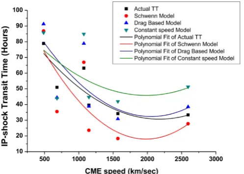
In this section, we compare the actual arrival time with transit time obtained by other models (Table 3). Here we are using three different shock arrival predic-tion models (1) constant Speed Model, (2) Drag Based Model (DBM) proposed by Vrsnak et al. (2013) and (3) transit time prediction model given by Schwenn

et al. (2005). The arrival time error for IP shock obtained from the models above with actual transit time are listed in Table 4. In the constant speed model, it has been predicted that CME travels the entire Sun Earth distance at the same speed (initial speed of CME) to reach at 1 AU. And also plot these different obtain transit time of IP-shocks in Figure 3. The Drag Based Model assumes that the CME speed dragged due to interaction of ICME and ambient solar wind. In DBM, the given parameters are: starting radial distance of CME (r0), CME speed at r0 (v0), asymptotic solar wind and drag parameter. The DBM tool is accessible in the website http://oh.geof.unizg.hr/index.php/en/spaceweather-tools. After putting all the values for reported CMEs, we have got the transit times at 1 AU. We have taken average ambient solar wind speed as 500 km/sec, which is the av-erage speed of plasma flow recorded by in-situ instrument. Schwenn et al. (2005) proposed a relationship between the arrival time and linear speed of CMEs as:

(

CME

)

203 20.77 ln rr

T = − ∗ V

[image:7.595.251.500.515.692.2]

where Trr is arrival time and VCME is linear speed of CME. In this case of arrival time of interplanetary shock, minimum transit time error is given by DBM model for four events (less than 6 hr).

(8)

[image:8.595.210.540.109.240.2]

Table 3. Transit time error for second order speed at final distances in second column and second order speed at 20 solar radii for all three reported CME events.

No. of Event Second-Order Speed (at Final Distance) Second-Order Speed (at 20 Solar Radii) 0.7 AU 0.6 AU 0.5 AU 0.7 AU 0.6 AU 0.5 AU

1 26.73 26.67 26.75 23.64 23.58 23.67

2 15.71 15.67 15.70 17.19 17.16 17.18

3 −18.44 −18.56 −18.42 −11.33 −11.43 −11.28

4 −0.27 −0.34 −0.25 2.60 2.54 2.62

5 −0.95 −1.12 −0.98 −7.51 −7.71 −7.60

6 7.29 7.23 7.28 7.30 7.25 7.30

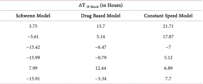
Table 4. Difference between the actual transit time and estimated transit time with vari-ous models (transit time error) for of IP shocks associated with selected CMEs.

∆T IP Shock (in Hours)

Schwenn Model Drag Based Model Constant Speed Model

3.75 15.7 21.71

−5.61 5.14 17.87

−15.42 −6.47 −7

−15.99 −0.79 5.12

7.99 12.44 6.89

−15.91 −3.34 7.7

4. Conclusion

[image:8.595.211.540.283.419.2]

(9)

dis-DOI: 10.4236/ijaa.2019.93014 199 International Journal of Astronomy and Astrophysics tances or at 20 solar radii.

Acknowledgements

We are grateful to Solar Geo-physical Data team, Kyoto and OMNI data team for their open data source policy. Authors are thankful to SOHO/LASCO CME catalogue (generated and maintained by CDAW data centre by NASA). We thank Prof. Bhuwan Joshi, USO, Physical Research Laboratory, Ahmedabad, and Pro. Hari Om Vats, scientist, Physical Research Laboratory, Ahmedabad India for his great support to us.

Conflicts of Interest

The authors declare no conflicts of interest regarding the publication of this pa-per.

References

[1] Vrsnak, B. and Gopalswamy, N. (2002) Influence of the Acceleration Drag on the Motion of Interplanetary Ejectas. Journal of Geophysical Research: Space Physics, 107, 1009. https://doi.org/10.1029/2001JA000120

[2] Vrsnak, B., Žic, T., Vrbanec, D., Temmer, M., Rollett, T., Möstl, C., Veronig, A., Čalogović, J., Dumbović, M., Lulić, S., Moon, Y.-J. and Shanmugaraju, A. (2013) Propagation of Interplanetary Coronal Mass Ejections: The Drag Based Model. So-lar Physics, 285, 295-315. https://doi.org/10.1007/s11207-012-0035-4

[3] Shanmugaraju, A. and Vršnak, B. (2014) Transit Time of Coronal Mass Ejections under Different Ambient Solar Wind Conditions. Solar Physics, 289, 339-349.

https://doi.org/10.1007/s11207-013-0322-8

[4] Manoharan, P.K. (2006) Evolution of Coronal Mass Ejections in the Inner Helios-phere: A Study Using White-Light and Scintillation Images. Solar Physics, 235, 345-368. https://doi.org/10.1007/s11207-006-0100-y

[5] Manoharan, P.K., Gopalswamy, N., Yashiro, S., Lara, A., Michalek, G. and Howard, R.A. (2004) Influence of Coronal Mass Ejection Interaction on Propagation of In-terplanetary Shocks. Journal of Geophysical Research: Space Physics, 109, A06109.

https://doi.org/10.1029/2003JA010300

[6] Gopalswamy, N., Lara, A., Manoharan, P.K. and Howard, R.A. (2005) An Empirical Model to Predict the 1-AU Arrival of Interplanetary Shocks. Advances in Space Re-search, 36, 2289-2294. https://doi.org/10.1016/j.asr.2004.07.014

[7] Gopalswamy, N., Lara, A., Yashiro, S., Kaiser, M.L. and Howard, R.A. (2001) Pre-dicting the 1-AU Arrival Times of Coronal Mass Ejections. Journal of Geophysical Research: Space Physics, 106, 29207-29217. https://doi.org/10.1029/2001JA000177

[8] Michalek, G., Gopalswamy, N., Lara, A. and Manoharan, P.K. (2004) Arrival Time of Halo Coronal Mass Ejections in the Vicinity of the Earth. Astronomy and Astro-physics, 423, 729-736.