Relativity: Towards a New Interpretation

ISSN Online: 2380-4335 ISSN Print: 2380-4327

DOI: 10.4236/jhepgc.2019.53041 Jul. 10, 2019 790 Journal of High Energy Physics, Gravitation and Cosmology

Relativity: Towards a New Interpretation

Carmine Cataldo

Independent Researcher, Battipaglia, Italy

Abstract

The aim of this paper essentially lies in attributing a new meaning, coherent with phenomenological reality, to several phenomena usually classified as re-lativistic, such as the alleged increase of the mean lifetime of muons and the gravitational redshift. According to the model herein proposed, all the relati-vistic equations preserve their validity, albeit with a different connotation. We consider a Simple-Harmonically Oscillating Universe, characterized by a null curvature parameter, postulating the existence of a further spatial dimension, not directly perceivable. Time is considered as being absolute, although in-struments and devices of whatever kind, commonly employed to measure it, may be significantly influenced by motion and gravity. The Planck Constant is regarded as a parameter, locally variable and subjected to a cyclic evolution. Time and space are treated as quantized physical quantities.

Keywords

Special Relativity, Lorentz Transformations, General Relativity, Cosmological Models, Black Holes, Schwarzschild Solution, Variable Planck Constant

1. Introduction

The paper consists, net of this short introduction, of 9 Sections or Paragraphs. In Paragraph 2, the well-known compatibility between General Relativity (from now onwards GR) and a Simple-Harmonically Oscillating Universe, flat and conventionally singular at t=0_{, is accurately discussed: in detail, starting} from the first Friedmann-Lemaître Equation, we carry out a step-by-step deriva-tion of the simple equaderiva-tion that describes the cyclic variaderiva-tion (over time) of the Scale Parameter (the radius, in our case).

In Paragraph 3, the existence of a further spatial dimension is postulated. The Universe is identified with a 4-Ball, the radius of which may evolve in accor-dance with the relation derived in the previous paragraph, and the concept of material point is definitively replaced by the one of material segment. In the light

How to cite this paper: Cataldo, C. (2019) Relativity: Towards a New Interpretation. Journal of High Energy Physics, Gravita-tion and Cosmology, 5, 790-849.

https://doi.org/10.4236/jhepgc.2019.53041

Received: May 21, 2019 Accepted: July 7, 2019 Published: July 10, 2019

Copyright © 2019 by author(s) and Scientific Research Publishing Inc. This work is licensed under the Creative Commons Attribution International License (CC BY 4.0).

http://creativecommons.org/licenses/by/4.0/

DOI: 10.4236/jhepgc.2019.53041 791 Journal of High Energy Physics, Gravitation and Cosmology of these assumptions, we firstly carry out an alternative deduction of the so-called Mass-Energy Equivalence, albeit with a different meaning: subsequently, by in-troducing a non-material term (which may be related to the so-called Quantum Potential), we obtain a rewriting of the Conservation of Energy. Finally, exploit-ing an opportune space quantization, we achieve the expression for so-called Relativistic Energy, the connotation of which, coherently with the aim of this paper, turns out to be undoubtedly distant from the norm.

In Paragraph 4, we address the Lorentz Transformations, backbone of Special Relativity (from now onwards SR). At this stage, we introduce more explicitly the absoluteness of time. In the light of this fundamental assumption, undenia-bly tough, we carry out, by exploiting the outcomes attained in the previous pa-ragraph, an unconventional derivation of the Lorentz Transformations, both in direct and inverse form. Obviously, the equations we obtain, although formally coinciding with the Lorentz Transformations, can no longer be considered as being relativistic (at least in the Einsteinian sense of the term) and acquire a meaning concretely different from the one usually ascribed to them.

In Paragraph 5, in order to provide a better understanding of some notewor-thy positions carried out in the second paragraph, we propose an alternative de-duction of the Friedmann-Lemaître Equations. At the end of the section, how-ever, the Metric Expansion/Contraction is manifestly and uncompromisingly considered as being an apparent phenomenon, related to the variability of the Planck Constant. In detail, by resorting to the Generalized Uncertainty Principle, we improve the quantization introduced in the second paragraph, so attaining the writing of the first Friedmann-Lemaître equation as a function of a time- dependent Planck “Constant”.

In Paragraph 6, we start dealing with Gravitation. Firstly, taking into account the results obtained in the previous paragraph, we definitively postulate a static scenario. Secondly, in order to ideally create Gravitational Singularities, we build a simple model entirely based on the redistribution of mass, the total amount of which is considered as being constant. By means of the above-mentioned model, we determine how space fabric is deformed by mass. Finally, we check the com-patibility between the hypothesized scenario and the quantization introduced in the second paragraph (and improved in the fifth).

DOI: 10.4236/jhepgc.2019.53041 792 Journal of High Energy Physics, Gravitation and Cosmology In Paragraph 8, we examine the well-known Schwarzschild Solution. Starting from a flat metric, obtained by exploiting the parameterization introduced in the previous paragraph, we initially carry out, by resorting to a preliminary Hil-bert-Like Approach, a conventional derivation of a Schwarzschild-Like Metric. Next, starting from the same initial flat metric, but following a completely dif-ferent line of reasoning, we deduce an infinite class of Schwarzschild-Like Solu-tions (including the metrics derived by Droste and Brillouin). At the end of the section, we briefly address the Gravitational Redshift, regarded as exclusively re-lated to the local variability of the Planck Constant.

In Paragraph 9, in the light of the image of the alleged Black Hole, placed at the heart of M87, recently captured by the Event Horizon Telescope, we initially provide a short outline of an interesting theory, fully coherent with GR, accord-ing to which the above-mentioned image may portray a so-called Eternally Col-lapsing Object (and not a Black Hole). Next, by introducing the concept of ve-locity as a complex vector, we propose a further explanation (non-relativistic, unlike the previous), compatible with the image in question, which may pe-remptorily exclude the existence of Black Holes (and Event Horizons).

2. The Oscillating Universe in General Relativity

According to Harrison’s classification [1], there are four main groups of Uni-form Cosmological Models compatible with GR: static, asymptotic, monotonic, and oscillatory.

Each of the above mentioned groups, in turn, may be subdivided into sub-groups or classes. We herein exclusively address the upper-bounded oscilla-tory class characterized by a flat (Euclidean) geometry: in particular, we will de-rive a Simple-Harmonically Oscillating Model, conventionally singular at t=0_.

2.1. Oscillatory Class with

k

= 0

For a uniform Universe, with the usual hypotheses of homogeneity and isotropy, we can write the first Friedmann-Lemaître Equation [2] [3] as follows:

(

)

2

2 2 2

d _{1 8π .}

d 3

R _{G c R kc}

t ρ

 _{ = + Λ −}  

  (2.1)

R represents the Scale Factor [3], G the Gravitational Constant, ρ the Density, Λ the so-called Cosmological Constant [3], k the Curvature Parameter [3], the value of which depends on the hypothesized geometry, and c the Speed of Light.

As is well known, if we denote with E Energy, with T the Thermodynamic Temperature, with S the Entropy, with p the Pressure, and with V the Volume, we can write:

dE T S p V= d − d . _(2.2) If we identify the evolution of the Universe with an isentropic process, from the previous Equations we obtain:

DOI: 10.4236/jhepgc.2019.53041 793 Journal of High Energy Physics, Gravitation and Cosmology According to Mass-Energy Equivalence [3][4], we have:

2_.

E Mc= _(2.4)

Obviously, we can write:

( )

d d d _{d .}

d d d d

M _{V V} V

t t t t

ρ

ρ ρ

= = + (2.5) Taking into account Equations (2.4) and (2.5), from Equation (2.3) we obtain:

2 d 2 d d _0,

d d d

V V

c V c p

t t t

ρ _ρ

+ + = (2.6)

2

d d _0.

d d

p V

V

t c t

ρ₊_ρ+  ₌

 

  (2.7)

Since we consider _V∝R3_{, with R≠0, we have:}

2 2

1 d 3 d _.

d d

V p R p

V t ρ c R t ρ c

 ₊ ₌  ₊ 

   

    (2.8)

From the last two Equations, we immediately deduce the so-called Fluid Equ-ation:

2 2

d 3 d _{3 .}

d d

R p R p

t R t c R c

ρ

ρ= = − _ρ+ _= − _ρ+ _

   

(2.9)

According to Zeldovich [5], the relation between pressure and density (the Equation of State) can be written as follows:

(

)

p= ν− ρc _(2.10) Evidently, the Universe is identified with a barotropic fluid (pressure exclu-sively depends on density). The value of ν, hypothesized as being constant, solely depends on the type of fluid we take into consideration (matter, radiation, rela-tivistic gas, dark energy, etc.): the general accepted values lie in the range 1≤ ≤ν 4 3 _[5].

From Equation (2.8), taking into account Equation (2.10), we obtain: d ₃ dR_.

R

ρ _ν

ρ = − (2.11)

As a consequence, if we denote with C the constant of integration, we can eas-ily deduce the following:

3 _.

Rν C

ρ = _(2.12)

Equation (2.1) can be evidently rewritten as follows:

2 3

2 3 2 2 2

d 8π 1 _.

d 3 3

R _{G R R c R kc}

t

ν ν

ρ −

 _{ = + Λ −}  

  (2.13)

By virtue of Equation (2.12), the underlying new constant can be now defined: 3

8π 8π _.

3 3

G R GC

Cν ν

ρ

= = (2.14)

DOI: 10.4236/jhepgc.2019.53041 794 Journal of High Energy Physics, Gravitation and Cosmology

2 2 3 1 2 2 2_.

3

R C R ν c R kc

ν −

= + Λ −

_(2.15)

Denoting with ω the Pulsation of the Oscillating Universe we want to de-scribe, we can carry out the following position involving the cosmological con-stant: 2 3 . c ω  

Λ = −  _{ } (2.16)

If we set k=0, by substituting Equation (2.16) in Equation (2.15), we finally obtain:

2 2 3 2 2_.

R C R ν R

ν − ω

= −

_(2.17)

From the previous equation, we can deduce as follows: 2 3

3 ₂

1 2

d _{1 ,}

d

R _{C R} R

t C ν ν ν ν ω − _ _ = _{−  }     (2.18) 3 ₂

1 ₂ 3

2

1 d _{d ,}

1

R _t

C R _R

C ν ν ν ν ω − _{ } =   − _ _   (2.19) 3 2 2 3 2 d

3 d . 2 1 R C t R C ν ν ν ν ω νω ω          _{ =}     − _ _   (2.20)

If we impose that the radius of curvature assumes a null value when t=0_, from the prior equation we can deduce:

3 2 ₃ arcsin , 2 R _t C ν ν ω _νω    _{ =}       (2.21)

(

)

sin 1 cos 3 ,

2 2

C C

Rν ν _νωt ν _νωt

ω ω

 

= _{ }= _ − _

  (2.22)

(

)

1 3

3

2 1 cos 3 .

2

C

R ν ν _νωt _ν

ω

 

=_{  } − _

  (2.23)

According to Equation (2.23), we have formally achieved a model of Universe belonging to the oscillatory class (“O Type” in Harrison’s Classification) [1].

From Equations (2.14) and (2.22), we immediately obtain:

(

)

2

3

3 3 1 _.

8π 4π 1 cos 3

C

GR G t

ν ν ω ρ νω = =

DOI: 10.4236/jhepgc.2019.53041 795 Journal of High Energy Physics, Gravitation and Cosmology Finally, by taking into account Equation (2.16), we can write the foregoing as follows:

(

)

2 ₁

. 4π 1 cos 3

c

G t

ρ

νω Λ

= −

− (2.25)

2.2. A Simple-Harmonically Oscillating Universe

If we set ν =1 3_{, from Equation (2.23) we obtain:}

( )

2 1 cos . 2

C

R ωt

ω

= _ − _{ (2.26)}

In other terms, we have found a simple-harmonically oscillating universe characterized by a variable density whose value, taking into account Equation (2.25), is provided by the following relation:

( )

2 ₁

. 4π 1 cos

c

G t

ρ

ω Λ

= −

− (2.27)

Denoting with A the Amplitude of the motion, taking into account Equation (2.26), we can immediately write:

1 3 2. 2

C

A= _{ω (2.28)}

If we set ω =t π 2_{, denoting with} R_m the mean radius, from Equations (2.26) and (2.28) we have:

π _.

2 m

R  = = _{ } A R (2.29)

By virtue of the previous, from Equation (2.27) we have:

( )

4π

m Rm c_G

ρ =ρ = −Λ _(2.30)

Evidently, taking into account Equations (2.28) and (2.29), Equation (2.26) acquires the following banal form:

( )

1 cos .

m

R R= _ − ωt _{ (2.31)}

Now, from Equation (2.12), since we have set ν =1 3, we can write: .

m m

R R

ρ =ρ _(2.32)

From Equations (2.14), (2.28) and (2.32) we have: 1 3

2 4π 4π _,

2 m 3 m 3 m

C G R G

R R

ρ

ω = = ρ = _(2.33)

(

)

3 2

2

2 π

3 m m _.

m

m

R G

R

R ρ ω

 

 

 

= _(2.34)

2.3. Particular Case: Further Positions

DOI: 10.4236/jhepgc.2019.53041 796 Journal of High Energy Physics, Gravitation and Cosmology 3

2_{π ,}

3

m m m

M = R ρ _(2.35)

.

m

R c

ω = _(2.36)

The position in Equation (2.35), at a first glance undoubtedly puzzling, will be at a later time easily understood when dealing with the concept of “Global Cen-tral Symmetry”.

From Equation (2.34), taking into account Equations (2.35) and (2.36), de-noting with Rs the so-called Schwarzschild Radius [3] [7], we can write:

(

)

2

2 m _.

m M G s m

R R M

c

= = (2.37) In the light of the outcomes so far achieved, we can evidently write the fol-lowing:

,

m

ct t

R

ω = =α _(2.38)

(

)

m

R R= − α _(2.39)

cos 1 ,

m

R R

α = − _(2.40)

d _{sin ,}

d

R

R c

t α

= =

_(2.41)

2

d _{cos 1 .}

d m m

R c R

R c

t ω α R R

  = = = _ − _  

_(2.42)

The beginning of a new cycle (t=0_{) occurs when the radius of curvature} as-sumes a null value. The problem related to the singularity [1] [8], herein not concretely addressed, may be solved by resorting to a quantization (see para-graph): in other terms, we should imagine a “Quantum Leap” (actually, anything but a novelty) [9] [10] so as to prevent the radius from concretely assuming a null value.

The evolution of the hypothesized Universe is evidently characterized by four consecutive phases: an accelerated expansion, a decelerated expansion, a decele-rated contraction, an acceledecele-rated contraction. All the above-mentioned phases have the same duration.

By taking into account Equations (2.38), (2.39) and (2.41), we can immediate-ly write the Hubble Parameter [11], commonly denoted by H, as follows:

2 2sin cos

1

2 2 _.

2sin ₂ tan

2

m m

m

R c c

H

R R R ct

R

α α

α

   

   

   

= = =

   

   

  _{ }

(2.43)

3. Introducing the 4

_{Spatial Dimension}

3.1. Mass-Energy “Equivalence”: Alternative Derivation

DOI: 10.4236/jhepgc.2019.53041 797 Journal of High Energy Physics, Gravitation and Cosmology (in other terms, a simple harmonic oscillator consisting of a mass and an ideal spring).

Denoting with m the mass of the above-mentioned point, taking into ac-count Equation (2.36), the Elastic Constant, denoted by ke, can be written as

follows:

2

2 _.

e

m

c

k m m

R

ω  

= =  

  (3.1)

Consequently, the Total (Mechanical) Energy, with obvious meaning of the notation, acquires the following form:

2 2

-point 1₂ 1₂ . m

R e m

E = k R = mc _(3.2)

Now, by solely modifying the amplitude of the motion, denoted by Rm′,

keeping the values of mass and pulsation constant, we can generalize Equa-tion (2.39) as follows:

(

)

(

)

]

]

R′=R R′ ′ α =R′ − α R′∈ R _(3.3)

From Equations (2.39) and (3.3) we have: .

m m

R R

R R

′ ′

= _(3.4)

At any given time, the value of R is obviously univocally determined by means of Equation (2.39), being Rm constant. On the contrary, the value of

R′_{, provided by Equation (3.3), clearly depends on the amplitude of the}

mo-tion (Rm′ ).

Taking into account Equations (3.1) and (3.4), the total energy of a materi-al point, the motion of which is described by Equation (3.3), acquires the fol-lowing form:

2 2

2 2 2

-point 1₂ 1₂ 1₂ .

m

R e m m

m

R R

E k R mc mc

R R

′

′

   ′

′

= = _{ } = _{ }

 

  (3.5)

The material point can now be replaced by a Material Homogeneous Segment (in other terms, it is as if we consider a spring, no longer ideal, with a length at rest equal to Rm). The length of the segment (R) evolves in accordance to

Equa-tion (2.39).

If we denote now with M the Mass of the Segment (the Linear Mass), the Linear Density can be banally defined as follows:

.

M M

R

= _(3.6)

Consequently, denoting with M′ _{the Mass of a Portion of Segment}

cha-racterized, at any given time, by a length equal to R′_{, we can write the}

fol-lowing:

,

R

M MR M

R ′

DOI: 10.4236/jhepgc.2019.53041 798 Journal of High Energy Physics, Gravitation and Cosmology .

M M

M

R R

′

= =

′ (3.8)

Equation (3.8) clearly shows how the linear density does not vary along the segment. As a consequence, taking into account Equations (3.5) and (3.7), the Energy related to an Infinitesimal Material Segment can be written as follows:

2 2 2

2 2 2

3

1 1

d d d d .

2 2 2

R R R Mc

E c M c M R R R

R R R

′

′ ′

  _′   _{′ ′ ′} = _{ } = _{ } =

    (3.9)

Taking now into account Equations (3.7) and (3.9), the final expression for the energy of a material segment, whose length, at any given time, is equal to

R′_{, acquires the underlying form:}

3 2

2 2

0

1 1

d .

6 6

R

R R R

E E Mc M c

R R

′ ′

′ ′

   

′ ′

= = _{ } = _{ }    

∫

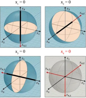
At this stage, it is necessary to introduce a Further Spatial Dimension [12]. The Universe we hypothesize is identifiable with a 4-Ball: the Radius, de-noted by R, evolves in accordance to Equation (2.39). The corresponding boundary, that may represent the space we are allowed to perceive (at rest) [6] [12], is a three-dimensional surface (a Hyper Sphere) described by the fol-lowing identity:

2 2 2 2 2

1 2 3 4 .

x +x +x +x =R _(3.11)

The 4-Ball is banally described by the following inequality:

2 2 2 2 2

1 2 3 4 .

x +x +x +x ≤R _(3.12)

Let us consider the point P+ _{defined as follows:}

(

)

P+ ₌ R _(3.13) Denoting with P− _{the antipode of P}+ _{(the point diametrically opposite),} we have:

(

)

P− _{= −}R _(3.14) We must now consider the straight line segment bordered by the points

P+ _{and P}−_.

Figure 1 provides the representations of the above-mentioned segment, by looking into the scenarios that arise from Equation (3.12) if we set equal to zero, one at a time, all the four coordinates.

If we set x4 =0, we obtain nothing but a single point (as shown in Figure

1). Therefore, we have to examine the three-dimensional scenarios that arise from the underlying identity:

0, 1,2,3.

i

x = i= _(3.15)

For example, we can set x1=0 (obviously, the same line of reasoning can be followed by setting x2 =0 and x3 =0). As a consequence, from Equa-tions (3.12), (3.13) and (3.14) we immediately obtain:

2 2 2 2

2 3 4 ,

DOI: 10.4236/jhepgc.2019.53041 799 Journal of High Energy Physics, Gravitation and Cosmology

Figure 1.Representations of a material segment.

(

)

1 0,0, ,

P+₌ R _(3.17)

(

)

1 0,0, .

P− _{= −}R _(3.18) Let us now consider the straight line segment bordered by the centre of the ball and the point defined by Equation (3.17). If the segment in question, the length of which evolves in accordance with (2.39), is provided with a mass equal to M, its energy can be immediately deduced from Equation (3.10) by setting R′ =R. Consequently, underlining how the same procedure can be obviously adopted for the point defined by Equation (3.18), we can write, with obvious meaning of the notation, as follows:

2

,1 ,1 1₆ ,

R R

E+ ₌E− ₌ Mc _(3.19)

2 1 R,1 R,1 R,1 1₃ .

E ₌E ₌E+ ₊E− ₌ Mc _(3.20) Generalizing, for the material segment, crossing the centre of the 4-Ball, characterized by a length equal to 2R and a mass equal to 2M, we have:

2

, , , 1₃ , 1,2,3.

i R i R i R i

E ₌E ₌E+ ₊E− ₌ Mc i_{= (3.21)} Finally, by superposition, we can easily write the total amount of energy related to the material segment bordered by the points defined by Equations (3.13) and (3.14):

3

2

1 i .

i

E E Mc

=

=

∑

DOI: 10.4236/jhepgc.2019.53041 800 Journal of High Energy Physics, Gravitation and Cosmology As far as our perception of reality is concerned, each point and its antipode are to be actually considered as being the same entity, since they both belong to the same straight line segment. In other terms, we can state that, according to our model, the Universe is characterized by a concrete Global Central Symmetry. [6] [12] [13]

3.2. The Conservation of Energy

Let us consider one amongst the scenarios defined by Equation (3.15). For ex-ample, we can set, once again, x1=0. Initially, the homogenous material seg-ment, bordered by the points P+ _{and P}− _{defined in Equations (3.17) and} (3.18), is characterized by a length equal to 2R and a mass equal to 2M. Let us suppose that the segment starts rotating around the centre of the 3-Ball defined by Equation (3.16).

If we impose the Conservation of Energy, the motion must necessarily en-tail modifications involving length and/or mass of the segment: otherwise the Kinetic Energy would be simply added to the energy defined by Equation (3.21), and the Total Energy could no longer be regarded as being constant. Obviously, the length of the segment in motion cannot increase: otherwise, the inequality in Equation (3.16) would be clearly violated (in other terms, the points P+ and P− _{would end up with being paradoxically placed beyond the boundary).}

Now, in order to find an equation that may express the conservation of energy, we must impose some conditions.

Firstly, we impose that the Tangential Speed of the endpoints (of the seg-ment), from now onwards denoted by v, cannot exceed the speed of light.

Secondly, we impose that the motion does not cause any linear density var-iations (this specific condition will be later legitimized): therefore, the value of the linear mass must keep on abiding by the simple rule established in Eq-uation (3.7).

Ultimately, according to our model, the motion may produce, concurrently, a loss of linear mass and a (symmetric) reduction of the length of the seg-ment.

If 2R′ _{represents the total length of the segment, denoting with I the}

Mo-ment of Inertia, we can write the Kinetic Energy as follows: 2

,1 1₂ .

k v

E I

R

  = _{ } ′

  (3.23)

If 2M′ _{represents the (reduced) mass of the segment (in motion), we have:}

(

)( )

1 _{2 2} 2 _.

12 3

I= M′ R′ = M R′ ′ _(3.24)

From the two previous Equations we immediately obtain: 2

,1 1₃ . k

E = M v′ _(3.25)

DOI: 10.4236/jhepgc.2019.53041 801 Journal of High Energy Physics, Gravitation and Cosmology the segment, since it is involved in the cyclic evolution described by Equation (3.3), is also provided with the following energy:

2 2

,1 ,1 ,1 1₃ ,1.

R R R R p

E E E M c E

R

+ −

′ ′ ′

′   _′ = + = _{ } =

  (3.26)

From Equations (3.25) and (3.26), taking into account the condition expressed in Equation (3.7), we obtain:

2 2

2 2 2 2

,1 ,1 1₃ 1₃ .

k p R R R

E E M v c M v c

R R R

  ′    ′  ′

′

+ =  +_{ } =  +_{ } 

   

   

    (3.27)

It is easy to verify how, since v cannot exceed the speed of light, when R′

approaches 0 (when the segment tends to completely lose its mass), Ek,1+Ep,1 tends to vanish. Therefore, in order to grant the conservation of energy, we need to introduce a further energetic term, denoted by Ew,1. Obviously, when

R′ =R _(when M′ =M _), E_w,1 must vanish; on the contrary, when R′

ap-proaches 0 (when the segment tends to completely lose its mass), Ew,1 must tend to the value in Equation (3.21). Moreover, since Ek,1+Ep,1 linearly de-pends on M′_{, we impose a linear dependence also between Ew,1 and} M′_.

Consequently, we have:

(

)

,1 1₃ .

w

E = M M c− ′ (3.28)

Taking into account Equations (3.21), (3.25), (3.26) and (3.28), we can finally write the conservation of energy, for the considered scenario (x1=0), as follows:

(

)

2

2 2 2 2

1 1₃ 1₃ 1₃ R 1₃ .

E Mc M v M c M M c

R

′  

′ ′ ′

= = + _{ } + −

  (3.29)

By multiplying by three all the members of the foregoing, taking into account Equation (3.22), we finally obtain the underlying relation:

(

)

2

2 2 2 2 _.

k p w

R

E Mc M v M c M M c E E E

R

′  

′ ′ ′

= = +_{ } + − = + +

  (3.30)

k

E represents the (real) kinetic energy, Ep the Potential (Background) Energy (related to the cyclic evolution of the Universe), Ew (a “non-material”

aliquot, which may be related to the so-called “Quantum Potential”) [14] [15], represents the energy needed to obtain the motion (to obtain the mass reduc-tion).

From Equation (3.30) we immediately deduce the underlying noteworthy identity:

2

2 2 R 2 _.

M c M v M c E

R

′  

′ = ′ +_{ } ′ = ′

  (3.31)

According to the definition of Lorentz Factor [16], we have:

2

1 _,

1 v

c

γ =

  −  _{ }

DOI: 10.4236/jhepgc.2019.53041 802 Journal of High Energy Physics, Gravitation and Cosmology 2

2 2 1

1 .

v

c β γ

  = = −  

  (3.33)

From Equation (3.31), exploiting Equations (3.32) and (3.33), we easily ob-tain:

2

2

1 v 1 R.

R R R

c β γ

 

′ = −_{ } = − =

  (3.34)

We have just found the relation between the tangential speed (of the end-points) and the Radial Extension (taking into account the symmetry) of the segment in motion.

From Equation (3.6), by virtue of the foregoing, we obtain:

2 .

1

M R _M M _M

R R _v

c

γ

= = =

′ ′ _{ } −  _{ }

(3.35)

Consequently, taking into account Equations (3.7), (3.8), (3.33), (3.34) and (3.35), the Specific Energies (the energies per unit of length) defined in Equation (3.30), can now be written, with obvious meaning of the notation, as follows:

2 2

2

2 ,

1

Mc Mc

E Mc

R _v

c

γ

= = =

′ _{ } −  _{ }

(3.36)

2

2 2 2

2

1

1 ,

k M v

E M c Mc

R β γ

′  

= = = −_{ }

′ _{ } (3.37)

2 2 2

2 ,

p R M c Mc

E

R R γ

′ ′

 

=_{ } =

′

  (3.38)

(

)

2 2

2

1 1 1 .

w M M c R M c

E Mc

M R R R γ

′ ′

   

=_ − _ =_ − _ = −

′ ′ ′ ′

    (3.39)

Therefore, by dividing both members of Equation (3.30) by R′_{, we obtain:}

,

k p w

E E= +E +E _(3.40)

(

)

2

2 2 2

2 2

1

1 Mc 1 .

Mc Mc Mc

γ γ

γ γ

 

= −_{ } + + −

  (3.41)

Denoting with E0 the Energy at Rest (R′ =R), provided by Equation (3.22), by virtue of the Equations (3.6), (3.36) and (3.39), we have:

2 2

0 Mc ,

E Mc

R

= = _(3.42)

(

)

2 2

0 1 0 w.

E=γMc =E + γ − Mc =E +E (3.43) Now, by dividing both members of Equation (3.31) by R′_{, taking into}

ac-count Equations (3.8) and (3.34), we obtain: 2

2 2

2 . Mc

DOI: 10.4236/jhepgc.2019.53041 803 Journal of High Energy Physics, Gravitation and Cosmology By multiplying both members of the foregoing equation by γ, taking into account Equation (3.36), we have:

2

2 2 Mc _,

Mc Mv

γ γ

γ

= + (3.45)

2

2 2

2

2 2 1 .

1 1

Mc Mv v

E Mc

c

v v

c c

 

= = + _{−  }

 

   

−_{ } −_{ }

   

(3.46)

3.3. “Relativistic Energy”: Punctual Mass and Space Quanta

In order to obtain the formal definition of the so-called Relativistic Energy, we have to impose a Space Quantization.

If R is regarded as a Primary Measurable Quantity [17], denoting with ∆Rmin the (Radial) Quantum of Space [18] (the value of which will be estimated at a later time), and with  an integer (obviously,  ≠0), we can write:

min.

R= ∆_ R _(3.47)

The Punctual (Three-Dimensional) Mass, denoted by m, can be defined as follows:

min.

m M R= ∆ _(3.48)

We can now finally legitimize the hypothesis of constancy of the linear density. From Equations (3.6) and (3.48), in fact, we can immediately deduce how the punctual mass is not influenced by the motion. In other terms, by virtue of the constancy of the linear density, m can be considered as being constant (and the misleading concept of Relativistic Mass can be definitively rejected).

Now, taking into account Equation (3.40), for a Material Point we have:

(

)

min min , , , .

m k p w k m p m w m

E = ∆E R = E +E +E ∆R =E +E +E _(3.49) By multiplying both members of Equation (3.41) by ∆Rmin, we have:

(

)

2

2 2 2

2 2

1

1 1 .

m mc

E γmc mc γ mc

γ γ

 

= =_ − _ + + −

  (3.50)

Now, by multiplying all the members of Equation (3.47) by ∆Rmin, we finally obtain the well-known relation for the Relativistic Energy [3] [4]:

2

2 2

2

2 2 1 .

1 1

m mc mv v

E mc

c

v v

c c

 

= = + _{−  }

 

   

−_{ } −_{ }

   

(3.51)

Denoting with pm the Momentum, with  the (Relativistic) Lagrangian,

and with  the Hamiltonian, we have:

2,

1

m mv

p

v c

=

  −  _{ }

DOI: 10.4236/jhepgc.2019.53041 804 Journal of High Energy Physics, Gravitation and Cosmology 2

2 1 v mc ,

c   = − −  _{ }

 (3.53)

Consequently, we can rewrite Equation (3.51) as follows: .

m m

E == p v− (3.55)

3.4. Towards a “New (Special) Relativity”

According to the results up to now obtained, what we perceive as being a (ma-terial) point may actually be a straight line (ma(ma-terial) segment crossing the cen-ter of the 4-Ball described by the inequality in Equation (3.12).

The endpoints represent all we are allowed to perceive of any segment. Cohe-rently with the hypothesized central symmetry, moreover, the endpoints are to be considered as being a unique entity (in a certain sense, they can be regarded as “entangled”).

The Uniform Linear Motion of a punctual mass may actually be a rotation (with a constant angular speed) of the corresponding material segment around the center of the 4-Ball. The rotation produce, concurrently, a loss of linear mass (although the value of the punctual mass is clearly preserved) and a (symmetric) reduction of the length: the new radial extension of the segment (half its length), denoted by R′_{, depends on the value of the tangential speed}

acquired by its endpoints (the constant speed that characterize the apparent linear uniform motion, denoted by v).

The relation between R′ _{and v is expressed by Equation (3.34).}

The Universe perceived by an observer involved in a linear uniform motion, characterized by a constant speed equal to v, is therefore described by the fol-lowing equality:

2 2 2 2 2

1 2 3 4 .

x +x +x +x =R′ _(3.56)

4. The Lorentz Transformations

The Lorentz Transformations can be considered, without any doubt, as the backbone of SR. Nonetheless, both the conventional derivation of the transfor-mations and the meaning commonly assigned to them have been often savagely criticized, to the extent that, despite an alleged empirical evidence, the whole SR theory, in several occasions, has been brought into question.

Firstly, it is worth underlining how, as Lorentz himself was forced to admit at a later time [19], the transformations had been already conceived, several years before the publication of the famous paper [16], by someone else [20]. Secondly, the work of Lorentz was anything but concretely linked to relativistic issues, at least in the Einsteinian sense of the term [3] [4]. Very simply, Lorentz’s aim fundamentally lay in finding some transformations able to formally make the well-known Maxwell Equations [21] (Maxwell, 1873) invariant. On this subject, moreover, it can be even proved how the Lorentz transformations are not the only ones able to preserve the formal validity of the Maxwell equations [22].

DOI: 10.4236/jhepgc.2019.53041 805 Journal of High Energy Physics, Gravitation and Cosmology meaning of symbols and signs, as follows:

2 ,

1

x vt x

v c

′+ ′ =

  −  _{ }

(4.1)

2

2. 1

vx t

c t

v c ′ ′ + =

  −  _{ }

(4.2)

The so-called Inverse Transformation [16] are usually written in the following form:

2 ,

1

x vt x

v c

− ′ =

  −  _{ }

(4.3)

2

2 . 1

vx t

c t

v c − ′ =

  −    

(4.4)

It is commonly said that, when the speed assumed by the mobile frame of ref-erence is far less than that of light, the Lorentz Transformations tend to the Ga-lilean ones. In other terms, according to the previous assertion, GaGa-lilean Relativ-ity should be interpreted as a particular case of the Einsteinian one. This is an erroneous conviction [23]. In fact, referring to the ratio that appears in the nu-merator of Equations (4.2) and (4.4), it is easy to understand how no limitation turns out to be imposed, respectively, on the variables x and x’. Therefore, since the above mentioned variables should be able to evidently assume arbitrarily large values, the ratio we have taken into consideration could even not tend to zero, so making de facto impossible a real identification of the Lorentz trans-formations with the Galilean ones [24]. As we are about to see, however, this misleading problem can be easily overcome by means of an alternative deriva-tion of the transformaderiva-tions, carried out by imposing the absoluteness of time.

4.1. The Lorentz Transformations: Alternative Derivation

In order to deduce the direct transformations, we will consider the scenario in

Figure 2.

The deduction will be carried out net of the symmetry.

We denote with O the origin of the Frame of Reference at Rest, and with O′

the origin of the Frame of Reference in Motion. At the beginning, obviously, O and O′ _{coincide. We have to hypothesize that when O}′ _{starts moving, with a}

constant speed equal to v, a signal is simultaneously sent from a source, that both the observer at rest and the one in motion will perceive as being punctual. The initial Angular Distance between the origins and the source is denoted by

DOI: 10.4236/jhepgc.2019.53041 806 Journal of High Energy Physics, Gravitation and Cosmology

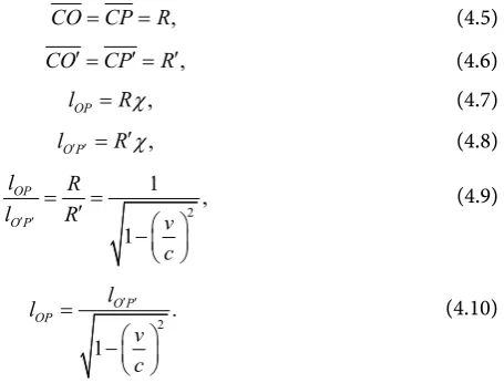
Figure 2.Direct transformations.

The signal is actually sent from each of the points that belong to the straight line segment bordered by the center of curvature, denoted by C, and P. The lat-ter represents the source as perceived by an observer at rest. The radial extension of any point at rest is evidently equal to the radius of the 4-Ball, denoted by R.

As soon as O′ _{starts moving, its radial extension, denoted by} R′_{, assumes}

the value provided by Equation (3.34). If we denote with lOP the arc bordered

by O and P, representing the distance at rest from the source, and with lO P′ ′ the arc bordered by O′ _{and P}′_{, which represents the distance between O}′ _and

the source as soon as the motion occurs, taking into account Equation (3.34), we can write the following:

,

CO CP R= = (4.5)

,

CO CP′= ′=R′ _(4.6)

,

OP

l =Rχ _(4.7)

,

O P

l ′ ′=R′χ (4.8)

2

1 _,

1

OP

O P

l R

l R _v

c ′ ′

= =

′ _{ } −  _{ }

(4.9)

2 .

1

O P OP l l

v c ′ ′

=

  −  _{ }

(4.10)

The coordinate of the light source as measured by the observer at rest, up until now denoted by lOP, can be replaced by x. After a certain time, denoted by t′,

the observer in motion intercepts the signal. Let’s denote with E′ _{the rendezvous}

point. Obviously, the time elapsed is equal to the time taken by light to cover the distance lE P′ ′. The above mentioned distance coincides with the coordinate of the light source, denoted by x′_{, as measured by the observer in motion as soon}

as the signal is received. We have: ,

OP

l =x _(4.11)

,

E P

l ′ ′ =x′ (4.12)

,

E P

l x

t

c c

′ ′ ′

DOI: 10.4236/jhepgc.2019.53041 807 Journal of High Energy Physics, Gravitation and Cosmology ,

O E

l ′ ′=vt′ (4.14)

.

O P E P O E

l ′ ′=l ′ ′+l ′ ′= +x vt′ ′ (4.15)

From Equations (4.10) and (4.15) we can immediately deduce (4.1), which represents the First Direct Lorentz Transformation.

If we divide the first and second member of Equation (4.1) by c, we obtain:

2. 1

x vt

x _{c c}

c _v

c

′ ′

+ =

  −  _{ }

(4.16)

The first member of the previous equation, that can be denoted by t, represents the time elapsed between the light signal emission and the moment in which the observer at rest succeeds in seeing it. From Equations (4.13) and (4.16) we can immediately obtain Equations (4.2), that represents the Second Direct Lorentz Transformation.

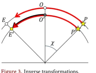
In order to deduce the inverse transformations, we will consider the scenario in Figure 3.

This time, referring to the bi-dimensional representation provided by Figure 3, we have to suppose that the occurs counterclockwise (once again, with a con-stant speed equal to v). Obviously, the Equations from (4.5) to (4.10) are still va-lid. We can serenely exploit the line of reasoning previously followed in deriving the direct transformations, being careful to switch the superscripts: from the point of view of the observer in motion, in fact, the one at rest, placed in O, seems to approach the light source (moving with a constant speed equal to v).

Therefore, we can now write the following: ,

OP

l =x′ _(4.17)

,

E P

l ′ ′=x (4.18)

,

E P

l x

t

c c

′ ′

= = _(4.19)

,

E O

l ′ ′ =vt (4.20)

.

O P E P E O

l ′ ′=l ′ ′−l ′ ′= −x vt (4.21)

From Equations (4.10) and (4.21) we can immediately deduce Equation (4.3), which represents the First Inverse Lorentz Transformation.

DOI: 10.4236/jhepgc.2019.53041 808 Journal of High Energy Physics, Gravitation and Cosmology If we divide the first and second member of Equation (4.3) by c, we obtain:

2 . 1

x vt

x _{c c}

c _v

c − ′

=

  −    

(4.22)

The first member of the previous equation, that can be denoted by t′_,

represents the time elapsed between the light signal emission and the moment in which the observer placed in O, actually at rest but considered as being in rela-tive motion towards the source, succeeds in seeing it. From Equations (4.21) and (4.22) we can immediately obtain Equation (4.4), which represents the Second Direct Lorentz Transformation.

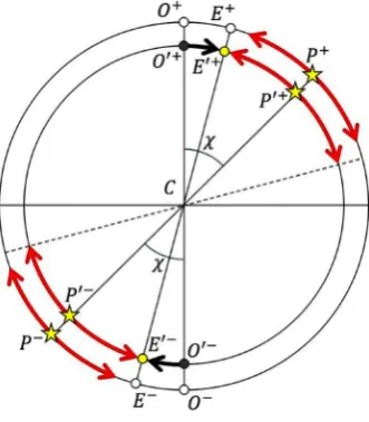
It is fundamental to underline that, if we take into account the symmetry, both the direct transformations and the inverse ones can be simultaneously applied to whatever point in motion with a constant speed equal to v: referring to Figure 4

(which represents just a modified version of the figure used to deduce the direct transformations), in fact, we can easily notice how, due to the symmetry, the light signals start not only from P+ _{and P′}+_{, but also from P}− _{and P′}−_, moving both clockwise and counterclockwise.

Very simply, the observer in motion travels towards the signal that propagates counterclockwise, so making possible the adoption of the direct transformations; simultaneously, the same observer moves away from the signal that propagates clockwise, so making possible the adoption of the inverse transformations.

4.2. Some Noteworthy Consequences

Firstly, referring to both the previously described scenarios, we can state that if the motion were suddenly stopped in E′_{, the traveler would be instantaneously}

dragged into E, and the signal, after a certain period of time, would be seen once again: in other terms, the observer would be involved in some sort of déjà-vu.

Secondly, we can state that the distance between the traveler and the light source undergoes a reduction as soon as the motion takes place: the higher the value of the speed, the higher the entity of the reduction. For example, re-ferring to the first of the two cases previously examined, we can state that the traveler is able to cover the distance lO P′ ′ by taking a time, denoted by tmob,

provided by the following relation:

.

O P mob l t

v ′ ′

= _(4.23)

However, once the traveler reaches the light source, the observer at rest be-lieves that the covered distance may be equal to lOP. As a consequence, from

the point of view of the observer at rest, the Apparent Speed of the traveler, denoted by vapp, is provided by the following relation:

.

OP OP

app

mob O P

l l

v v

t l ′ ′

DOI: 10.4236/jhepgc.2019.53041 809 Journal of High Energy Physics, Gravitation and Cosmology

Figure 4.Symmetry.

From Equation (4.24), by taking into account Equation (4.9), we can im-mediately write the following:

2.

1

app v

v

v c

=

  −  _{ }

(4.25)

Coherently with the domain of the relativistic factor, the Real Speed, that keeps on being denoted by v, can never equate that of light. On the contrary, the virtual speed, that we have denoted with vapp, tends to infinity when the

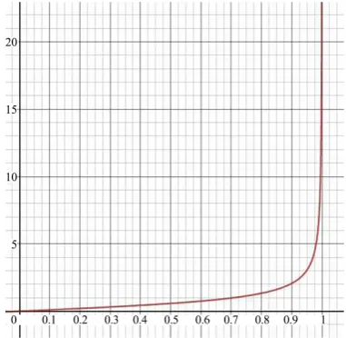
real speed tends to that of light. This result is qualitatively described by Fig-ure 5, in which the x-coordinate represents the ratio between the real speed and that of light (β), and the y-coordinate represents the correspondent value of the virtual speed, in number of times that of light.

As a consequence, an observer at rest will measure, in any given case, a speed greater than the real one. Obviously, from Equation (4.25) it is possible to easily deduce the relation that expresses the virtual speed, the one meas-ured by the observer at rest, as a function of the real one:

2.

1

app

app v v

v c

=

  +    

(4.26)

Let’s now choose a “destination”. Generalizing Equation (4.10), if we de-note with l the distance at rest from the point that we have to reach, and with

mob

l the corresponding Reduced Distance (the distance that a traveler, who starts moving with a speed equal to v, should actually cover in order to reach the destination), we have:

2

1 .

mob v

l l

c  

= _{−  }

DOI: 10.4236/jhepgc.2019.53041 810 Journal of High Energy Physics, Gravitation and Cosmology

Figure 5.Apparent speed as a function of real speed.

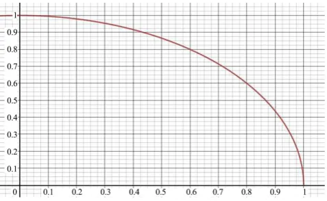
This result is qualitatively described by Figure 6 in which the x-coordinate represents, once again, the ratio between the real speed and that of light (β), and the y-coordinate represents the correspondent value of the ratio between the reduced distance and the one measured at rest.

4.3. The Alleged Increase of the Lifetime of Muons (Short

Account)

Amongst the so-called “proofs of Special Relativity”, the alleged increase of the lifetime of muons stands out. In the light of the results up to now ob-tained, the phenomenon may be easily explained avoiding time dilations. Muons evidently succeed in covering a distance clearly not compatible with their mean lifetime: this is irrefutable. On the one hand, we could admit that time, for muons, starts slowing down due to the high value of their speed; on the other hand, and for the same reason, we may also imagine that, for muons, both the radial extension and the distances undergo a reduction (the pheno-menon, according to our theory, is no longer restricted to the direction of the motion). In the latter case, the speed perceived by an observer at rest is great-er than what it really is, and time, clearly, does not undgreat-ergo any dilation whatsoever.

5. Again on the Friedmann-Lemaître Equations

DOI: 10.4236/jhepgc.2019.53041 811 Journal of High Energy Physics, Gravitation and Cosmology

Figure 6.Reduced distance as a function of real speed.

In this section we carry out an alternative deduction (without resorting to GR) of the Friedmann-Lemaître Equations [2]. It is nothing but an “inverse procedure”, the finality of which exclusively lies in clarifying some positions, such as the one in Equation (2.35), we have previously exploited in building our model.

5.1. The Friedmann-Lemaître Equations: Alternative Derivation

By virtue of the global (central) symmetry [6] [12] [13] so far hypothesized, denoting with M half the mass of the Universe, we can define the density as follows:

3.

2_π 3

M R

ρ= _(5.1)

Coherently with Equation (2.35), taking into account Equation (2.39), if

m

M represents the mass when R R= m, from the prior equation we obtain:

( )

2

2

2 3

3 . 2_π

4π

3 ₂

m m

m m

m m

m

c

M R

R

c R R

M

ρ =ρ = = _(5.2)

Coherently with Equation (2.37), we can now carry out the following posi-tion:

2 . 2m m

R c G

M

= _(5.3)

From the previous position, taking into account Equation (5.2), we obtain: 2

2

3 . 4πm m

c R G

ρ = (5.4)

We can now define the cosmological constant as follows:

2 3 .

m

R

DOI: 10.4236/jhepgc.2019.53041 812 Journal of High Energy Physics, Gravitation and Cosmology Taking into account the foregoing, from Equation (5.4) we recover Equa-tion (2.30).

Now, denoting with p the pressure, and with σ the Surface Tension (which must be clearly considered as being constant), we can write the well-known Young-Laplace Equation [25] as follows:

2 .

p R

σ

= _(5.6)

From the foregoing, by virtue of Equation (2.10), we can write:

( ) (

)

( )

d 1 d ₁ d _0.

dt 2 dt pR c dt R

σ _{= = ν− ρ =}

(5.7)

From the previous, we deduce Equation (2.32) or, equivalently, the follow-ing:

.

m m

R R

ρ= ρ _(5.8)

According to our hypotheses, moreover, we have:

( )

(

)

( )

d ₁ d _0,

dt pV dt V

ν _{= ν− ρ} ν _{= (5.9)}

,

m m

Vν Vν

ρ =ρ _(5.10)

3 3 _.

m m

Rν Rν

ρ =ρ _(5.11)

By carrying out a banal comparison between Equations (5.8) and (5.11), we can finally set ν =1 3_{. Consequently, from Equation (2.10) we immediately} obtain:

2

2 _.

3

p= − ρc (5.12)

From Equations (5.2) and (5.8) we immediately obtain: 2

3 _,

4π

m m

m

R c

R G RR

ρ

ρ

2 _4π . 3

m

c G

RR =

ρ

From Equations (2.40 and (2.41) we have:

(

)

2 2 2 2 2

2

1 cos 2 .

m m

R R

R c c c

R R

α

= − = −

_(5.15)

If R≠0_{, from the previous, by virtue of Equations (5.5) and (5.14), we} have:

2 ₂ 2 _{2 2}

2

8π

2 ,

3 m 3

m

R c R c c G

R R R RR ρ

  _{+ =}  ₋Λ _{= =}

   

   

(5.16)

(

)

2

2 2

d _{1 8π .}

d 3

R _{G c R}

t

ρ

 _{ = + Λ}

 

DOI: 10.4236/jhepgc.2019.53041 813 Journal of High Energy Physics, Gravitation and Cosmology Evidently, the previous equation is nothing but Equation (2.1) with k=0. Now, Equation (5.15) can be easily rearranged as follows:

2 2

2 2

2

2 1 .

m m m

c R R

R R c

R R R

  = _ − _+

 

_(5.18)

From the foregoing, by virtue of Equations (2.42) and (5.5), if R≠0 _we have:

2 2

2 2 2

2

2 2 ,

3

m

R c

R RR c RR R

R

Λ

= + = −

_(5.19)

2 ₂

2 .

3

R R c

R R

  _{= −}Λ

   

(5.20)

From Equations (5.12) and (5.16) we obtain:

2 ₂

2 4π _, 3

R c _{G p}

R c

  ₋Λ _{= −}

   

(5.21)

2 2 2

2 2

2

2 2 8π

2 .

3 3

R _c R R _c G _p

R R R c

     

− Λ = + − Λ = −

     

     

(5.22)

From the previous, by taking into account Equation (5.20), we finally ob-tain the usual writing of the Second Friedmann-Lemaître Equation [2] [3]:

2 2

2 8π

2R R c Gp.

R R c

 

+_{ } − Λ = −

 

(5.23)

5.2. The Metric Expansion/Contraction as an Apparent

Phenomenon

Actually, we consider the variations of cosmological distances as being an ap-parent phenomenon: in other terms, we postulate that the amount of space be-tween whatever couple of points remains the same with the passing of time (on this subject, it could be worth bearing in mind how Hubble himself started bringing into question the relation between the Redshift and the Recessional Velocity of Astronomical Objects) [26].

More precisely, we hypothesize that the so-called Cosmological Redshift may banally related to the conservation of energy.

As is well known, the energy of a Quantum of Light can be expressed as the product between the value of its frequency and the Plank Constant.

On the one hand, as an alternative to the conventional interpretation of the cosmological redshift, we could accept that, in travelling through the interstellar vacuum, light may somehow “get tired”, so losing part of its energy [27] [28] [29].

DOI: 10.4236/jhepgc.2019.53041 814 Journal of High Energy Physics, Gravitation and Cosmology In the latter case, evidently, all the cosmological equations can be rewritten as a function a Plank Parameter.

On this subject, it can be proved that, according to the Generalized Uncer-tainty Principle, ∆Rmin in Equation (3.47) can be expressed as follows [17]:

min 2 P.

R α′

∆ = (5.24) In the previous, P represents the so-called Planck Length and α′ a

con-stant.

There are several methods to estimate the value of α′ _{[33] [34] [35] [36]: in}

any case, however, we obtain α′ ≅1. Consequently, from Equations (3.47) and (5.24), making explicit the expression of P and setting α′ =1, we obtain:

min 2 3 .

G

R R

c

= ∆ =  (5.25)

From the previous, taking into account Equation (2.43), we can easily deduce: 2

2

2 1 _.

4

R _H h

R h

   

= =  

 

   

(5.26)

Therefore, Equation (5.17) can be rewritten, by resorting to the foregoing, as follows:

(

)

2

2 2

d _{4 8π .}

d 3

h _{G c h}

t

ρ

 _{ = + Λ}

 

  (5.27)

Beyond doubt, the possible variability of the Planck constant could still sound like a shocking hypothesis: nonetheless, it is worth bearing in mind how several physical quantities, initially considered as being constant, have been later classi-fied as variables. The Hubble constant faced exactly this fate, and quite soon it was downgraded, so to say, to the rank of parameter (the value of which is still under investigation) [37] [38] [39].

6. Gravitation: A Simple Model

In the light of what specified in the sub-paragraph 5.2, Rm and Mm can be

conventionally considered, respectively, as the real values of radius and mass. Replacing, for convenience, Rm with Rs, and Mm with Mtot (half the

real mass of the Universe, coherently with the symmetry), we now can rewrite Equation (2.37):

2 2 tot_.

s GM

R c

= (6.1)

Obviously, Equations (3.11) and (3.12) assume the following form:

2 2 2 2 2

1 2 3 4 s,

x +x +x +x =R _(6.2)

2 2 2 2 2

1 2 3 4 s.

x +x +x +x ≤R _(6.3)

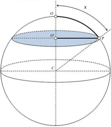
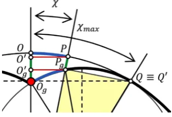
DOI: 10.4236/jhepgc.2019.53041 815 Journal of High Energy Physics, Gravitation and Cosmology which taken as origin, placed on the hyper-surface defined in Equation (6.2), and with O′ _{the centre of the so-called Measured Circumference, to which P}

belongs. Both O and O′ _{are considered as lying on} x₄. The angular distance between O and P, as perceived by an ideal observer placed in C, is denoted by

χ.

The arc bordered by O and P, denoted by Rp, represents the so-called

Proper Radius (the measured distance between the above-mentioned points). We have:

( )

p s

R χ =Rχ _(6.4)

The straight-line segment bordered by O′ _{and P, denoted by Rc or X,}

represents the so-called Predicted (or Forecast) Radius (the ratio between the perimeter of the measured circumference and 2π). We have:

( )

( )

c s

R χ =X χ =R χ _(6.5)

From the previous we immediately deduce:

arcsin .

s X R

χ= _ _

  (6.6)

Consequently, taking into account Equation (6.4), we have:

2 d

d d .

1

p s

s

X

R R

X R χ

= =

 

−  

 

(6.7)

The scenario is qualitative depicted in Figure 7.

At this point, for the hyper-surface defined in Equation (6.2), the so-called Friedmann-Lemaître-Robertson-Walker Metric (with k=1) [2] [3] can be written: