Lights and shadows : multi wavelength analysis of young stellar objects and their protoplanetary discs

(1)

MULTI-WAVELENGTH ANALYSIS OF YOUNG STELLAR

OBJECTS AND THEIR PROTOPLANETARY DISCS

Laura Rigon

A Thesis Submitted for the Degree of PhD

at the

University of St Andrews

2016

Full metadata for this item is available in

St Andrews Research Repository

at:

http://research-repository.st-andrews.ac.uk/

Please use this identifier to cite or link to this item:

http://hdl.handle.net/10023/8646

This item is protected by original copyright

(2)

Lights and Shadows

Multi-wavelength analysis of young stellar objects

and their protoplanetary discs

by

Laura Rigon

This thesis is submitted for the degree of

Doctor of Philosopy in Astrophysics at the University of St Andrews

(3)

(4)

Declaration

I, Laura Rigon, hereby certify that this thesis, which is approximately 45,000 words in

length, has been written by me, or principally by myself in collaboration with others as

acknowledged, that it is the record of work carried out by me and that it has not been

submitted in any previous application for a higher degree.

I was admitted as a research student in January 2012 and as a candidate for the degree

of PhD in January 2012; the higher study for which this is a record was carried out in the

University of St Andrews between 2012 and 2015.

Date Signature of candidate

I hereby certify that the candidate has fulfilled the conditions of the Resolution and

Regulations appropriate for the degree of PhD in the University of St Andrews and that

the candidate is qualified to submit this thesis in application for that degree.

(5)

(6)

Copyright Agreement

In submitting this thesis to the University of St Andrews I understand that I am giving

permission for it to be made available for use in accordance with the regulations of the

University Library for the time being in force, subject to any copyright vested in the work

not being affected thereby. I also understand that the title and the abstract will be

pub-lished, and that a copy of the work may be made and supplied to any bona fide library

or research worker, that my thesis will be electronically accessible for personal or research

use unless exempt by award of an embargo as requested below, and that the library has

the right to migrate my thesis into new electronic forms as required to ensure continued

access to the thesis. I have obtained any third-party copyright permissions that may be

required in order to allow such access and migration, or have requested the appropriate

embargo below.

The following is an agreed request by candidate and supervisor regarding the electronic

publication of this thesis: no embargo on print copy, no embargo on electronic copy.

Date Signature of candidate

(7)

(8)

Abstract

Stars form from the collapse of molecular clouds and evolve in an environment rich in gas and dust before becoming Main Sequence stars. During this phase, characterised by the presence of a protoplanetary disc, stars manifest changes in their structure and

luminosity. This thesis performs a multi-wavelength analysis, from optical to mm range, on a sample of young stars (YSOs), mainly Classical T Tauri (CTTS). The purpose is to

have a comprehension of both star and disc evolution in YSOs.

Optical and infrared fluxes are used to study stellar variability and its relation with the protoplanetary disc. Longer wavelength, in the mm range, are used instead to investigate

the evolution of the disc, in terms of dust growth.

The optical variability, quantified through pooled sigma, is visible both in magnitude amplitudes and changes over time. Time series analysis applied on the more variable stars

finds the presence of quasi periodicity, with periods between two weeks and a month, interpreted either as eclipsing material in the disc happening on a non-regular basis, or as

a consequence of star-disc interaction via magnetic field lines.

The variability of YSOs is confirmed also in infrared, even if with lower amplitude. No strong correlations are found between optical and infrared variability, which implies a

different cause or a time shift in the two events. By using a toy model to explore their origin, I find that infrared variations are likely to stem from emissions in the inner disc.

The evolution of discs in terms of dust growth is analysed using the slope of the spectral

energy distribution (SED), and by applying a detailed correction for wind emission and optical depth effects, specific for each star. The further comparison with a radiative

(9)

(10)

Collaboration statement

This thesis was written entirely by me, but some parts were developed in collaborations with other authors.

Chapter 3 is part of a paper in preparation ”Long-term variability of T Tauri stars

using WASP” by L. Rigon, A. Scholz, D. Anderson and R. West. Both the Chapter and

the paper make use of some proprietary data of the SuperWASP consortium, but they were then analysed entirely by me. D. Anderson and R. West provided important information

regarding the meaning of the errors in the photometric data, necessary for the analysis of the variability.

Chapter 5 uses some proprietary data of images observed and reduced by J. Greaves at

the Green Bank Telescope and C. Chandler at the Very Large Telescope. In Section 5.8 the BETAgrid, a radiative transfer model developed by P. Woitke and M. Min, is used to make

a comparison between observational results and models. Section 5.9, instead, uses the radiative transfer model ProDiMo not only to make a comparison with the observational

results, but also to derive the effects of model parameters on the slope of the SED. This last Section is also part of the paper”Consistent dust and gas models for protoplanetary

disks. I. Disk shape, dust settling, opacities, and PAHs” by P.Woitke and the entire

DIANA consortium, of which I am a member. With respect to the paper, the analysis in this thesis uses a different wavelength interval, and Figs 5.15 to 5.17, initially made by P.

(11)

(12)

Acknowledgements

I would like to thank Peter Woitke and Jane Greaves, who offered me the opportunity to come to St Andrews and pursue this PhD. A great thank you to Aleks Scholz, who took over the supervision in the second year and made me appreciate and enjoy my research.

I am grateful to him for all I have learned for the last two years, and for his constant support and constructive suggestions to improve my work. I would like to thank all the

students and postdocs I shared time with during these years, and in particular John for his precious advice to improve my IDL plots, and Claire for helping out with the proofreading of two chapters.

Outside the School, I would like to acknowledge the entire DIANA group, and in particular Inga Kamp for her useful suggestions during my three-day visit at the Kapteyn

(13)

(14)

“Zwei Dinge erf¨ullen das Gem¨ut

mit immer neuer und zunehmender

Bewunderung und Ehrfurcht,

je ¨ofter und anhaltender

sich das Nachdenken damit besch¨aftigt:

der bestirnte Himmel ¨uber mir

und das moralische Gesetz in mir.”

Immanuel Kant

“Two things fill the mind

with ever-increasing wonder and awe,

the more often and steadily

the mind of thought is drawn to them:

the starry heavens above me

(15)

(16)

List of Figures

1.1 Classification of YSOs on the basis of the gradient of the SED, between 2 and 25 µm (Lada, 1987). . . 6

1.2 Horizontal structure of a typical protoplanetary disc, whose host star has M = 1−2 M⊙ and T=4000 K. The picture highlights regions at different

distances from the host star and corresponding wavelength ranges used for their detectability. Adapted from Carmona (2010). . . 17

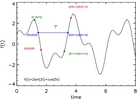
2.1 For each lagτ a set of pairs (f(t), f(t+τ) can be defined. In this example τ = 2. . . 29

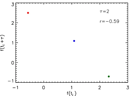
2.2 The pairs (f(ti), f(ti+τ)) are used to derive the correlation coefficient rτ for the lag τ. The example refers to the previous function, where τ = 2. Data are clearly anticorrelated in this case. . . 30

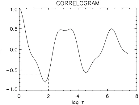
2.3 The correlogram shows that the best correlation is achieved when τ is be-tween 2.5 and 3.5 or after an inter cycle, i.e. at 6.28, equivalent to 2π. In the current exampler =−0.59 when τ = 2. . . 31

3.1 Lightcurves of LkHa 326 (left) and LkHa 327 (right). In red are highlighted the discarded data points, as explained in Section 3.2.1. . . 39

3.2 Mean magnitude versus standard deviation for the sample stars (asterisks) and the comparison stars (open circles). . . 42

3.3 Example of each type of pooled sigma, as described in Table 3.3. . . 45

3.4 Left: The plot shows, for each star, the slope of the best straight line that fits the pooled sigma plot versus maximum pooled sigma. In purple triangles are stars from group A, in blue circles group B (see text sect. 3.3.1). Right:

Slope versus maximum pooled sigma for a sample of 81 Class II stars in Taurus, taken from Table 7 in the survey by Luhman et al. (2010). Symbols are like before. . . 49

3.5 Differences between the percentages of stars in group A, B and A+B avail-able in DIANA and the comparison samples. . . 52

3.6 The diagram shows the DIANA and comparison samples in the slope-maxpooledsigma space. . . 52

(21)

ber 2011. . . 56

3.9 Folded lightcurve for CQ Tau between 9th December 2006 and 19th Febru-ary 2007. . . 56

3.10 Folded lightcurve for CW Tau between 8th November 2009 and 18th Jan-uary 2010. . . 57

3.11 Folded lightcurve for DO Tau between 25th September 2006 and 19th Jan-uary 2007 (left) and between 2nd October 2011 and 20th November 2011 (right). . . 58

3.12 Folded lightcurve for Haro 6-13 between 19th September and 18th Novem-ber 2011. . . 59

3.13 Lightcurve and folded lightcurve of RW Aur over the entire timescale, be-tween 27th July 2004 and 11th February 2011. . . 60

3.14 Lightcurve of LkHa 327 between July 2004 and December 2007 (left) and, not folded, between 10th September 2006 and 19th January 2007 (right). . 61

3.15 Magnitude variations on the 19thOctober 2011. Variations are clearly larger than photometric errors. . . 62

3.16 AA Tau lightcurve, not folded, between 19th _{and 25}th _{September 2011} (l.h.s), and between 19th and 24th October 2011 (r.h.s). . . 62

3.17 AA Tau lightcurve folded on 5-day period, between 19th and 25th October 2011 (l.h.s), and between 31st _{October 2011 and 13}th _{November 2011 (}_r.h.s_{). 63}

3.18 AA Tau lightcurve folded on 5-day period between 19th _{October and 3}rd November 2011 (l.h.s), and between 19th October and 13rd November 2011 (r.h.s). . . 63

3.19 Magnitude variations on the 25th_{August 2004. Variations are clearly larger} than photometric errors.. . . 64

3.20 CW Tau lightcurve folded on 10-day period between 20th August and 7th September 2004. . . 64

3.21 Magnitude variations on 3rd _{February 2009. . . 65}

3.22 DO Tau lightcurve folded on 8-day period between 8th and 21st August 2004. 65

3.23 Same plot as in Fig. 3.4, where in open squares there are single stars, in filled squares binary stars. . . 66

3.24 TheKS test shows that multiple (in blue) and single stars (in red) have the same distribution with respect to slope and max pooledsigma. D = 0.22 and D= 0.25 respectively,Dc=0.48. . . 67

3.25 σmax or S versus inclination available for only 19 stars in our sample. In triangle stars from group A, in filled circles stars from group B (see text). i=0◦

for face-on discs, i=90◦

(22)

3.26 max pooledsigma (left) and slope (right) versus spectral type, rmax = 0.02, rslope = −0.18. In triangles stars from group A, in filled circles stars from group B (see text, sect. 3.3.1). . . 69

3.27 max pooledsigma (left) and slope (right) versus α3.4−₄_.₅_µm. In triangles

stars from group A, in filled circles stars from group B (see text, sect.3.3.1). rmax = 0.43,rslope= 0.51 rc = 0.33. . . 72

3.28 max pooledsigma (left) and slope (right) versusα24−₇₀_µm. In triangles stars

from group A, in filled circles stars from group B (see text, sect. 3.3.1). rmax =−0.33,rslope =−0.25,rc = 0.48. . . 73

3.29 max pooledsigma (left) and slope (right) versus αU−_B. In triangles stars

from group A, in filled circles stars from group B. rmax =−0.69, rslope = −0.73 and rc = 0.60. Stars leftwards the dash-dotted line are accretors, rightwards are non accretors. . . 74

3.30 max pooledsigma (left) and slope (right) versusαN U V−B. In triangles stars from group A, in filled circles stars from group B.rmax = 0.82,rslope = 0.19, rc = 0.88. . . 75

3.31 Max pooled sigma and slope versus accretion rate derived from Hαemission. In triangles stars from group A, in filled circles stars from group B.rmax= −0.25, rslope =−0.25, rc = 0.53. . . 76

3.32 αU−B versus soft X-rays flux. The correlation coefficientr= 0.74 is greater than the critical valuerc= 0.71. . . 76

3.33 Top: Hard X-rays,rslope =−0.16,rmax =−0.22. Bottom: Correlation with Soft X-rays, rslope = 0.01,rmax =−0.14. The critical value is rc = 0.43 in both cases. . . 77

4.1 The diagram shows wherePk is positive or negative. In this example it is assumed that the mean i-magnitude is 4 and the mean j-magnitude is 6. . 88

4.2 Left: Histograms of the S.I. values in bands W1-W2. In green the full sample, in blue the reduced one. Right: Histograms of the S.I. values in bands W3-W4. In both diagrams the threshold between non-variable and variable stars is at 0.9, as defined by Rebull et al. (2014), and represented through the dashed red line. . . 89

4.3 Same histograms as in the previous figure, but here the absolute values of the S.I. are shown. In this study it was absolute value that was considered a more accurate indication of variability, as explained in section 4.3.1. . . . 89

(23)

solid line is the best fit for the variable stars, having S.I. above 0.9. The dotted lines represent the thresholds in S.I. andχ2. The Pearson correlation coefficient is 0.78 in W1 and 0.76 in W2, with a critical value of 0.40. In all bands, there is a good correlation for variable objects between the two parameters. . . 93

4.6 S.I. in bands W3 and W4 versusχ2 for band W3 (left) and W4 (right). The dotted line is the best fit for the variable stars, having S.I. above 0.9. The dotted lines represent the thresholds in S.I. andχ2. The Pearson correlation coefficient is 0.85 in W3 and 0.90 in W4 with a critical value of 0.41. In all bands, there is a good correlation for variable objects between the two parameters. . . 93

4.7 Comparison between the optical and infrared amplitude of variations for each star. The x−axis shows variations in each infrared WISE band, the y−axis shows variations in optical. . . 95

4.8 χ2 _{in band W3 and W4 compared to slope. In both diagrams, group A is}

colour-coded in purple, group B in blue. The critical value isrc = 0.37, and the correlation coefficients are printed at the bottom right of each figure. . . 95

4.9 S.I. in each pair of bands compared to slope. In all diagrams, group A is colour-coded in purple, group B in blue. The critical value isrc = 0.37, and the correlation coefficients are printed at the bottom right of each figure. . . 96

4.10 Histograms showing the number of stars vs slope of the fitted line, computed in the colour-magnitude diagrams. The dashed line divides negative from positive values. There is a clear prevalence of negative slopes. . . 97

4.11 Colour-magnitude diagrams in bands W1 and W2. The red arrow shows the direction of the extinction law for comparison. . . 98

4.12 Colour gradient versus inclination. The correlation coefficient is r = 0.04 and the critical value is rc = 0.48. Correlation coefficient for only negative gradients: r =0.29, rc = 0.55. . . 99

4.13 SEDs of some stars in our sample. Photosphere model in solid line, WISE infrared emissions in colours. . . 102

4.14 SED of AA Tau. The dashed line represents the emission from a hot spot having 50% of the stellar surface and T=7000 K. . . 104

4.15 Left: Histograms of the S.I. values in bands W1-W2. Right: Histograms of the S.I. values in bands W3-W4. The red dashed line represents the threshold between non variable and variable stars, as defined by Rebull et al. (2014). . . 109

(24)

4.17 Histogram showing the number of stars vs the slope of the fitted line in the colour-magnitude diagram, W1-W2 vs W1. The dashed line divides negative from positive values. There is a clear prevalence of negative slopes like in the DIANA sample. . . 111

5.1 Plots of discs with cm data. All discs have new data, either from VLA or GBT, except TCha. In red is highlighted the final flux, after subtracting the average correction for free-free emission, for all discs showing wind emission. All other discs not showing wind emission are in Appendix H. The dash-dotted line represents wind emission, the dash-dotted line is the linear fit through data between 1.2 mm and 1 cm. . . 138

5.2 Discs without cm data. In red is highlighted the final flux, after subtracting the average correction for free-free emission, for those discs showing wind emission. All other discs not showing wind emission are in Appendix H. The dash-dotted line represents wind emission. . . 139

5.3 α1.3−_7mm (red) or α₁_.₃−_{10 mm} (blue) versus log flux at 7 mm/1 cm (left) or

at 1.3 mm (right). The dash-dotted line represents the value ofα for grains in the interstellar medium. . . 141

5.4 ∆ correction as a function of Rd and τ. The density profile exponent is p=1, inclination θ= 60◦

and the temperature profile exponent q=0.56. . . . 149

5.5 ∆ correction as a function of p and τ. The outer radius is Rd=100 AU, inclination θ= 60◦

and the temperature profile exponent q=0.56. . . 152

5.6 Comparison between αSED and αBeckwith for ∆ computed at 1.3mm and two different inclinations, colour-coded in mean disc temperature< Td>. . 164

5.7 Comparison between αSED and αBeckwith for ∆ computed at 1.3 mm and two different inclinations, colour-coded in dust size exponentapow. . . 166

5.8 Comparison between αSED and αBeckwith for ∆ computed at 1.3 mm and two different inclinations. . . 167

5.9 Transition radius r1 versus ∆ correction for face-on discs, at 1.3 mm (left

hand side) and 3 mm (right hand side). . . 170

5.10 Transition radius r1 versus ∆ correction for inclinationθ= 60◦, at 1.3 mm

(left hand side) and 3 mm (right hand side). . . 170

5.11 Dependance of dust opacity, from 0.1µm to 1 cm, on different grain pa-rameters: minimum and maximum size (top row), dust grain distribution (bottom left) and chemical composition (bottom right). . . 174

5.12 Zoom of previous plots at λ≥1 mm . . . 174

(25)

and cm range (right), for Rd =100 AU (red triangles) and 600 AU (blue asterisks). The reference model is in green. . . 176

5.15 Midplane dust temperature on the midplane at 30 AU versus mm-slope (left) and cm slope (right). The correlation coefficient is r = 0.78 in the mm range and r= 0.66 in the cm range. The critical value is rc=0.58. All depicted models have the same dust opacity, hence the sameβ. . . 177

5.16 Midplane dust temperature on the midplane at 50 AU versus mm-slope (left) and cm slope (right). The correlation coefficient is r = 0.78 in the mm range and r= 0.63 in the cm range. The critical value is rc=0.58. All depicted models have the same dust opacity, hence the sameβ. . . 177

5.17 Variations to the SED slope, in the mm- and cm-range, caused by different disc and dust parameters with respect to the reference model (red dot). . . 179

A.1 Pooled sigma plots of stars in Chapter 3. . . 195

B.1 Entire lightcurves of stars in groups A and B, from 2004 until 2011. . . 198

C.1 Daily magnitude variations on CQTau can be negligible, as on the 16th January 2007 (l.h.s.), or more pronounced as on the 18th January 2007 (r.h.s.) . . . 200

C.2 Magnitude variations on the 15th January 2010 for Haro 6-13 (l.h.s.). Vari-ations can reach one magnitude in one day, but are affected by large pho-tometric errors, because the source is very faint. Magnitude variations on the 30th November 2009 for IQ Tau (r.h.s.). Variations are small and do not exceed half a magnitude, but are still larger than photometric errors. . 200

C.3 Magnitude variations on the 22th July 2006 for RU Lup (l.h.s.). Variations on the 20th October 2007 for RWAur (r.h.s.). . . 200

D.1 Same as Fig. 3.2, where in red is highlighted CQ Tau and in blue the comparison, non variable star J053505.04+243705.4. . . 202

D.2 Variation on the 18th January 2007 for CQ Tau and the comparison star. . 202

D.3 Variations between 29th January and 18th Februar 2007 for CQ Tau and the comparison star. . . 202

E.1 SEDs of the remaining stars in Fig. 4.13. Photosphere model in solid line, WISE infrared emissions in colours. . . 206

F.1 Colour-magnitude diagrams for the remaining stars in Fig. 4.11. . . 210

(26)

List of Tables

1.1 Differences between small and giant molecular clouds. From Hartmann (2009) and references therin. . . 2

1.2 List of the 85 objects, part of the DIANA database. . . 20

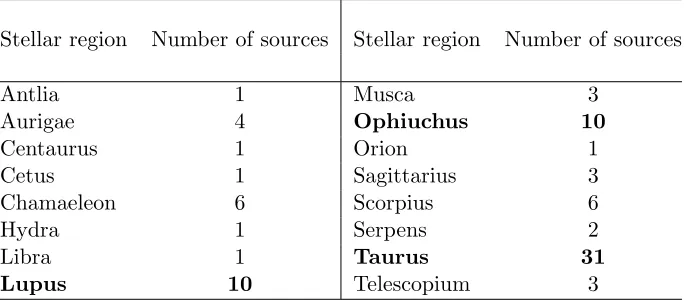
1.3 Stellar regions and corresponding number of sources of the DIANA sample. 20

3.1 Data sample. In bold are highlighted stars that belong to group A, stars from group B are underlined. (See text, Sect. 3.3.1). (1)Bouvier et al. (1999), (2)Muzerolle et al. (2003), (3)Andrews & Williams (2007a), (4)Natta & Whitney (2000), (5)Kitamura et al. (2002), (6)Piétu et al. (2011), (7)Mc-Cabe et al. (2011), (8)Monin & Bouvier (2000), (9)Panić & Hogerheijde (2009), (10)Stempels et al. (2007), (11)Eisner et al. (2007), (12)Isella et al. (2010), (13)Qi et al. (2006), (14)Simon et al. (2000), (15)White & Ghez (2001), (16)Woitas et al. (2001), (17)Barsony et al. (2003), (18)Tamazian et al. (2002), (19)Correia et al. (2006), (20)Welch et al. (2004), (21)Muze-rolle et al. (2001b), (22)Andrews & Williams (2007b), (a)Herczeg & Hillen-brand (2014), (c)Hernández et al. (2004), (d)Kenyon & Hartmann (1995), (e)Bouvier & Appenzeller (1992), (f)Luhman et al. (2010), (g)Casali & Eiroa (1996), (h)Fernandez et al. (1995), (i)Hughes et al. (1994), (l)Köhler et al. (2000), (m)Torres et al. (2009), (n)Houk & Smith-Moore (1988), (o)Cohen & Kuhi (1979), (p)Grankin et al. (2007), (q)Andrews & Williams (2005) . . . 41

3.2 Noisy nights removed from the original fits files in the entire sample. The long semester between 2007 and 2008 was removed only in LkHa 326 and LkHa 327. See sect. 3.2. . . 42

3.3 Different types of pooled sigma curves, their main features, percentages and an example star. . . 44

3.4 Pooled sigma values for each star and each time subset. The maximum pooled sigma and the slope of the fitted line are in the last two columns. In bold, stars from group A; underlined, stars from group B (see text). . . . 48

3.5 Statistic on slope and max pooled sigma in DIANA and in the comparison sample. Q represents quantile at different percentages of data points. . . . 50

(27)

al. (2012), (2) Luhman et al. (2010), (3) Evans et al. (2003), (4) Meyer et al. (2006), (5) Rebull et al. (2010), (6) Ducati (2002), (7) Morel & Magnenat (1978), (8) Kharchenko (2001), (9) Mermilliod (2006) , (10) Mermilliod et al. (1997), (11) Ofek (2008), (12) Richmond (2007), (13) de Winter et al. (2001). . . 71

4.1 S.I. for bands W1-W2, W3-W4 and W2-W3 and χ2 for each single band. The highest absolute value in each column is highlighted in bold, the lowest one is underlined. The purple background is for stars in group A, the yellow one for stars in group B (see chapter 3). . . 92

4.2 WISE magnitude and flux zeropoints . . . 100

4.3 Areas of hot spots at different temperatures causing the observed variations in W1 and W2. The full list is in Appendix G. Stars whose hotspots resulted to be larger than the stellar surface are in the Table. . . 104

4.4 Disc areas, in units of stellar area, responsible for the additional infrared emissions in bands W1 and W2, from a source at 850 K. The asterisks denote stars whose radii are known from the literature, in all other cases R∗ = 1.8 R⊙. . . 107

4.5 Areas, in units of stellar area using Beckwith’s model. . . 108

5.1 Fluxes from the literature. Underlined discs have only data from the lit-erature, and not from VLA or GBT. (1)Mannings (1994), (2)Sandell et al. (2011), (3)Skinner et al. (1993), (4)Andrews & Williams (2005), (5)Beck-with et al. (1990), (6)Guilloteau et al. (2011), (7)Rodmann et al. (2006), (8)Alonso-Albi et al. (2009), (9)Mannings & Sargent (1997), (10)Testi et al. (2001), (11)Ricci et al. (2010), (12)Isella et al. (2009), (13)Isella et al. (2010), (14)Kitamura et al. (2002), (15)Koerner et al. (1995), (16)Lom-men et al. (2010), (17)Ubach et al. (2012), (18)Nuernberger et al. (1997), (19)Lommen et al. (2007), (20)Cortes et al. (2009), (21)Carpenter et al. (2005), (22)Lommen et al. (2009), (23)Henning et al. (1993), (24)Akeson et al. (1998), (25)Osterloh & Beckwith (1995), (26)Andr´e & Montmerle (1994), (27)Dai et al. (2010), (28)Jenness et al. (2002) . . . 124

5.2 New fluxes from GBT or VLA. . . 125

5.3 Stars used to compute the average wind correction at 7 mm and 1 cm, and their respective free-free components with errors. . . 130

5.4 Slope of the SED in different wavelength intervals without and with wi nd correction. The power law used to correct for free-free emission is in the third column. Depending on the available data, fluxes at 3 mm can be represented by fluxes at 2 mm, 2.7 mm, 2.8 mm, 3.3 mm, 3.4 mm or 3.6 mm. Peculiar cases are marked with an asterisk and described in Section 5.5.1. . 136

(28)

5.6 Values of κλ for each wavelength used in the ∆ computation. . . 146

5.7 Minimum and maximum ∆ values at the shortest (1.3 mm) and longest (1 cm) wavelength, for discs atθ= 0◦ _and _θ_{= 60}◦ _{inclination. . . 148}

5.8 Illustrative ∆ values, in ascending order for each Rd, at 7 mm forθ= 60◦

, p= 1. . . 150

5.9 Values of optical depth τ, dust mass M (in M⊙), transition radius r₁ and

outer radius Rd (in AU), for different values of disc inclination and wave-length, when ∆≥0.5. The density power law index is p = 1 in all cases. When ∆<0.5 no values are reported. . . 150

5.10 Illustrative ∆ values, in ascending order, at 7 mm forθ= 60◦

,Rd= 100 AU. 153

5.11 Values of optical depthτ, dust massM (in solar masses), density power law indexp and transition radiusr1 (in AU), for different values of disc

inclina-tion and wavelength, when when ∆≥0.5. The outer radius isRd=100 AU in all cases. When ∆<0.5 no values are reported. . . 153

5.12 Values of α, after applying the wind correction when necessary, β, and βcorr corrected for optically thick effects. Dust masses from Beckwith et al. (1990), p= 1,θ= 30◦

. In italics: for discs having α <2,β is taken equals to 0. The asterisk (*) is for stars where α is between 1.3-7 mm. Radii are from: 1Rodmann et al. 2006, 2Ricci et al. 2010,3Cieza et al. 2011,4Ratzka 2008,5Lommen et al. 2009,6Dutrey et al. 1994,7Sipos et al. 2009,8ALMA Partnership et al. 2015. In Ricci et al. (2010), radii are from Kitamura et al. (2002) and Andrews & Williams (2007a), but an average was taken. . . 157

5.13 Comparison, for cases where βcorrected from the previous table is available, betweenβfrom this work and from the literature. The asterisk∗

means that βwas corrected for optically thick regions, even if with different choices of ∆. textitBECK90: Beckwith et al. (1990),ROD2006: Rodmann et al. (2006),

LO0709: Lommen et al. (2007) or Lommen et al. (2009), Ricci2010: Ricci et al. (2010), UB2012: Ubach et al. (2012), ALMA: ALMA Partnership et al. (2015). . . 158

5.14 Comparison between ∆, and respective β, computed at λ=1.3 mm and λ=7 mm/1 cm. In both cases 76% of the stars haveβ <1. . . 159

5.15 Complete list and values of parameters in the BETAgrid. . . 161

5.16 Fixed and variable parameters in the BETAgrid. . . 162

5.17 ∆ values, in ascending order, at 1.3 mm and θ = 60◦_{, corresponding disc}

parameters and SED slopes. . . 168

5.18 Parameters of the reference model used in ProDiMo. . . 172

5.19 . . . 178

(29)

(30)

1

Introduction

The formation of stars is a process which requires between 106_{to 10}7_{years to complete, but}

even before burning hydrogen in its core and qualifying as a “main sequence star”, a

pro-tostar is already observable, initially in far infrared and later also at optical wavelengths.

During the pre main sequence evolution the pre-stellar objects pass through several phases

and experience changes, not only in their structure, but also in their surrounding. In

par-ticular, variations in their luminosity are observed at different wavelengths, and formation

of planets are likely to happen around them.

This thesis aims to study young stellar objects (YSO) at various wavelengths, from

optical to centimeter range, and to analyse the light emitted from both the star and the

disc. The purpose is to understand the origin of the luminosity variability, in optical

and infrared, and how much it is related to the disc structure. The emission at longer

wavelength is used to infer the level of evolution of discs, in terms of dust grain growth.

(31)

stars (Section 1.1), highlighting the main features of low mass stars (Section 1.2 and 1.3)

and more massive ones (Section 1.4). Characteristics of discs forming around them

(Sec-tion 1.5) and mechanisms by which tiny dust grains grow into larger objects (Sec(Sec-tion 1.6)

are also presented. The final part of the Introduction focusses on the data sample used,

and the contribution of this thesis as part of the DIANA project (Section 1.7).

1.1 Formation of Young Stellar Objects

Star formation is known to begin in molecular clouds (e.g. Zuckerman & Palmer (1974);

Burton (1976)), made of gas, mainly molecular hydrogen but also carbon dioxide, and

dust. Dust is an important component, because it protects molecules from dissociation

due to ultraviolet (UV) radiation, and at the same time offers a medium for molecules

likeH2 to form. There are two types of molecular clouds: giant molecular clouds (GMC),

like Orion; and small molecular clouds (SMC), like Taurus, Auriga and Ophiuchus. They

differ in mass, density, size and temperature in the Galaxy, as shown in Table 1.1:

SMC GMC

Mass <104_M

⊙ 104

−₆

M⊙

Density 10−19/−20_{g cm}−3 ₁₀−19/−20_{g cm}−3

Size 10-50 pc ≈100 pc

Temperature 10-20K 50-100 K

Table 1.1: Differences between small and giant molecular clouds. From Hartmann (2009) and references therin.

GMCs and SMCs do not have uniform density, but present smaller structures like

cores and clumps, which have increasing density and temperature, and decreasing size and

mass compared to the larger molecular cloud. It is in these smaller and denser regions,

having diameters not larger than 10 pc and masses between 103_-104_M

⊙ (e.g. reviews

by Cernicharo (1991); Williams et al. (2000)), that the collapse begins, giving origin to

the formation of stars. Low mass stars can form in both GMC and SMC, whereas most

massive stars are more likely to be found in GMC.

Several models have been proposed as mechanism to trigger the initial process of star

formation, like for example turbulence, collisions of molecular clouds (Scoville et al., 1986)

(32)

1.1. Formation of Young Stellar Objects

developed by Elmegreen & Lada (1977), has been recently confirmed by some authors

(Chiaki et al., 2012), while others did not find any evidence between supernova remnants

and star forming regions (Desai et al., 2010). Concerning the formation of molecular

clouds, among the mechanisms proposed there are gravitational instability in the galactic

disc (e.g Elmegreen, 1979; Balbus, 1988); converging flows, valid for clouds up to 104M⊙

as described in Dobbs et al. (2014); and spiral shocks (Bonnell et al., 2013).

Independently of the initial causes, when the mass is greater than a critical value,

called the Jeans Mass, the cloud begins to collapse. The Jeans Mass, MJ, is defined as

follows:

MJ = 1.6 s 10 T K 3 cm−3

n

M⊙ (1.1)

where T is the temperature and n is the number density. MJ can be several order of

magnitude smaller than the total cloud mass, implying that molecular clouds would not be

observable so extensively, because they would collapse much earlier as soon as their mass

exceeds MJ. For this reason there must be some mechanisms to counteract gravity, like

thermal gas pressure , turbulence (Norman & Silk, 1980; Larson, 1981), magnetic fields

(Chandrasekhar & Fermi, 1953; Spitzer, 1968; Mouschovias, 1976) and rotation (Field,

1978). Turbulence and magnetic fields seem to be the main cause in larger clouds, while

thermal pressure would play a role in small cores (Larson, 2003).

According to Larson (1969), for a typical core in a SMC having T ≈ 10 K, ρ =

10−19_{g cm}−3_,_M _{= 1 M}

⊙and size comprised between 0.1 and 0.4 pc the process of collapse

can be divided into a number of steps, where the main ones are described below.

1. “Isothermal phase”: in the initial phase the cloud collapses in free fall, and while

the density is below 10−13_{g cm}−3 _{the gravitational energy liberated is free to escape.}

The duration of this phase is defined by the free-fall time:

τf f = r

3π

32Gρ (1.2)

which is ≈ 105 yrs. During the contraction of the molecular cloud, the density increases first in the centre rather than in the outer regions.

2. “Adiabatic phase”: when the density rises above 10−13_{g cm}−3 _{the medium becomes}

(33)

they can contrast the collapse, and a core in quasi hydrostatic equilibrium forms:

the protostar.

3. “Formation of the second core”: once the temperature is above 2000 K the molecular

hydrogen begins to dissociate, pressure drops and the core collapses even further.

Since the energy is used for the dissociation of molecules, this process happen nearly

in isothermal conditions. When all molecules are dissociated, temperature and

pres-sure rise again and stop the collapse of the core. Density is now≈10−₂

g cm−₃

, but

the mass is still small,≈10−2_M

⊙.

4. “Accretion phase”: The core of the protostar is now in hydrostatic equilibrium, while

most material is still accreting onto its surface. The luminosity of the protostar is

given by the conversion into radiation of the gravitational energy produced during

the shock on its surface. This phase corresponds to Class 0, described in the next

section.

The further evolution depends on the mass of the protostars, which can be divided

into two groups: low mass protostars, having M ≤ 3M⊙; and high mass ones, having

M >3M⊙. More massive protostars begin to burn hydrogen while they are still accreting

matter. In low mass protostars, instead, the accretion stops before they reach the main

sequence, where hydrogen is burnt, and the luminosity comes from the gravitational energy

liberated during the contraction that is still ongoing. The duration of this process is set

by the Kelvin-Helmoltz timescale:

τKH ≈ GM∗2

R∗L∗

(1.3)

Low mass stars in the pre-main sequence phase are called T Tauri stars, after their

prototype T Tau in the constellation of Taurus, and they will be the main subject of this

thesis, especially in Chapter 3 and 4. Chapter 5 will include, instead, also some more

(34)

1.2. T Tauri stars

1.2 T Tauri stars

T Tauri stars are low mass stars, having M ≤ 2M⊙ and Spectral Type F to M, which

means they are relatively cold, with surface temperatures between 2500 and 7000 K. They

exhibit luminosity variations; ultraviolet (UV), optical and infrared (IR) excess; present

inverse P-Cygni profile in emission lines, which are a signature of infalling matter, and

have strong magnetic fields of the order of 1-3 kG (Johns-Krull et al., 1999). The magnetic

field is a consequence of the structure of these stars, which are totally or almost totally

convective, and is generated by the motion of plasma.

T Tauri stars pass through four phases during their evolution to the main sequence.

They are called Class 0, I, II and III, and happen during the Kelvin-Helmoltz time, i.e.

when there is already the presence of a protostar in the molecular cloud and the luminosity

is generated by the release of gravitational energy. The difference among the classes was

determined on the basis of the spectral index of the spectral energy distribution (SED)

in the near-mid infrared, between 2 and 25µm (Lada & Wilking, 1984; Lada, 1987). The

SED represents flux as a function of wavelength, and the spectral index α is defined as

the slope of the SED between two wavelengths λ1 andλ2, in a log-log plot:

α= logλ1Fλ1 −logλ2Fλ2

logλ1−logλ2

(1.4)

where Fλ is the flux per unit wavelength. The initial classification by Lada (1987)

com-prised only Class I, II and III. Subsequently, when observations were extended to longer

wavelengths, a new class was introduced, called Class 0 (Andre et al., 1993), because

from an evolutionary perspective it occurs before the Class I phase. The four classes are

described below and depicted in Fig. 1.1:

• Class 0 During Class 0 objects are completely enshrouded by the molecular cloud

that the only emission is in the very far infrared, and they do not emit any light

in optical. This phase lasts for about 105yrs; the accretion is high, at a rate of 10−₅

M⊙yr −₁

and the radius of the envelope is of the order of 104_AU;

• Class IDuring this phase the central star is still embedded in the molecular cloud,

although some visible light is detectable. The SED is characterised by a rising

(35)

the spectral index was α ≥ −0.3, while now “true Class I” have α > 0.3, while

objects having −0.3 ≤ α < 0.3 are called “flat-spectrum” sources (Greene et al.,

1994). The timescale is longer than in Class 0, being ≈106yrs; accretion decreases to 10−6_M

⊙yr−1 and the radius shrinks to 103AU;

• Class II In this phase, which lasts ≈ 106₋₁₀7_{yrs, the emission from the central}

star is detectable clearly, but the star is still surrounded by a disc of dust and gas,

called protoplanetary disc. The infrared excess is less pronounced, and consequently

the spectral index becomes negative: −1.6≤α <−0.3.

• Class III In the last phase, stars do not have a disc anymore and the SED shows

only the emission from the photosphere, with a steep negative spectral index, being

[image:35.595.99.467.344.649.2]

α <−1.6.

Figure 1.1: Classification of YSOs on the basis of the gradient of the SED, between 2 and 25 µm (Lada, 1987).

This classification can be biassed by inclination, especially for edge-on discs, where a

Class I object could be erroneously identified as Class 0 (Robitaille et al., 2006). During

(36)

1.3. Properties of T Tauri stars

still present, but shows a large gap in the middle, most likely caused by ongoing planet

formation, identifiable by lack of infrared excess below 10µm. These objects are called

Transitional Discs (Strom et al., 1989).

Since Class II objects are still surrounded by a disc, they are of particular interest in

studying the process of star and planet formation, and in particular the effects of accreting

matter on the stellar luminosity and the process of dust growth, which will be developed

in the next chapters.

1.3 Properties of T Tauri stars

1.3.1 Magnetospheric accretion

Magnetospheric accretion is nowadays a well accepted model to explain the main features

of T Tauri stars, like UV, optical and IR excess, and inverse P-Cygni profile in emission

lines. Previous models, like the Boundary Layer model (Lynden-Bell & Pringle, 1974) or

wind models (Hartmann et al., 1982, 1990; Natta & Giovanardi, 1990), failed to explain

some of these features. The Boundary Layer model describes the star as surrounded by

a disc which extends almost to the stellar surface, except for a thin layer. If on one

hand it could explain the UV and IR excess, on the other one it could not account for

the inverse P-Cygni profile or the shape of the SED of many CTTS. Concerning wind

models, instead, even if wind is a component of T Tauri stars and these models could

explain the P-Cygni profile, they could not account for the inverse P-cygni profile, and

had difficulties in reproducing spectral lines with very faint or blushifted absorption, as

described in Alencar (2007).

These discrepancies were overcome by the Magnetospheric Accretion model (Hartmann

et al., 1994; Muzerolle et al., 1998, 2001a; Shu et al., 1994), where, unlike the Boundary

Layer model, the star accretes matter through a disc which is truncated at a few stellar

radii from the star (Camenzind, 1990; Koenigl, 1991). The disc truncation is caused by

the strong stellar magnetic field generated by the motion of charged particles inside the

star. Once the material accreting along the disc reaches its inner part, it will fall onto

the star following the magnetic field lines. The material falls onto the star at free-fall

velocity, causing the formation of an accretion shock, which in turn can explain the UV

(37)

as disc wind instead, in order to reduce the stellar angular momentum and allow other

material to accrete onto the star.

One of the tracers of accretion is the equivalent width of the Hαline in emission, which

corrisponds to the transition from the third to the second quantum level in the hydrogen

atom. The kinetic energy liberated during accretion is high enough to excite atoms and

produce emission lines. Hα is one of the most easily detectable, because its emission is in

the red part of the optical spectrum, at 6563 ˚A.

On the basis of the accretion rate, T Tauri stars can be divided into two classes:

classical T Tauri stars (CTTS), which are high accretors having an accretion rate of the

order of 10−8/−9_M

⊙yr−1 (Ingleby et al., 2013), and weak T Tauri (WTTS), which are

very low accretors where accretion is not detectable. One of the thresholds between these

two classes is given by the equivalent width (EW) of the Hα line in the Balmer series,

where EW>10 ˚A for CTTS and EW<10 ˚A for WTTS.

Since accretion is related to the presence of a disc, CTTS partially correspond to

Class II objects and WTTS to Class III. The two definitions, however, are not completely

interchangeable, because there are stars which own a disc, but do not accrete.

1.3.2 Luminosity variability

Optical variability was the first feature that characterised the discovery T Tauri stars in

the early 1940s (Joy, 1942, 1945), and more recent observations highlighted that changes

in luminosity happen also in infrared (Skrutskie et al., 1996; Carpenter et al., 2001, 2002;

Rebull et al., 2014; Cody et al., 2014). Optical and infrared variability in CTTS will be

extensively described and analysed in Chapter 3 and 4 respectively, therefore here only a

summary of their main properties will be given.

Variations appear in a wide range of types, from strictly periodic to completely

ape-riodic, the last case being more difficult to be interpreted. For the optical variability a

number of explanations have been provided and, among the most accredited, there are

cool and hot spots, and circumstellar variations (Herbst et al., 1994; Carpenter et al.,

2002; Bouvier et al., 2003). Cool spots are the equivalent of Sun spots, i.e. they are colder

regions with respect to the surrounding stellar surface, and for this reason appear to be

(38)

1.3. Properties of T Tauri stars

as the rotation period of the star. Hot spots, on the other hand, are related to

accre-tion and correspond to the regions on the stellar surface where material accreting from

the disc, through magnetic field lines, interacts with the star. The sudden conversion of

gravitational energy into thermal energy makes them appear brighter. They occur on a

less regular basis. Further, cool spots are related only to the stellar activity, while hot

spots are due to the presence of the protoplanetary disc and its interaction with the star.

Circumstellar variations are also related to the presence of the disc and its rotation. If

the disc presents an irregular and warped shape, especially in the inner edge, and is seen

almost edge-on, the host star will be sometimes more and sometimes less exposed to the

observer, with consequent changes in its apparent luminosity. This seems to be one of the

causes for AATau optical variability (Bouvier et al., 2003).

Cool and hot spots were claimed to explain also the near infrared variability (Carpenter

et al., 2001, 2002), but according to more recent studies (Flaherty et al., 2013) the effect

of hot spots is only indirect, and possibly other mechanisms in the disc are involved, such

as changes in the structure and height of the inner rim, explained also through disc wind

emission (Bans & K¨onigl, 2012). Since observation in mid and far infrared have been

achieved only for the past two decades, this kind of variability, and its connection with the

optical one, is still currently being investigated in the literature. In this context, simple

models will be developed and discussed in Chapter 4 to analyse the effect of hot spots and

disc emission.

1.3.3 Jets, outflows and winds

Jets and winds are typical features of T Tauri stars, which are observed throughout their

evolution and are responsible for mass loss in young stars. Their origin is still controversial,

but they seem to be related to accretion and magnetic field, either in the star or the disc.

By removing angular momentum they would allow the star to continue accreting matter

from the disc without spinning above the break-up rotation speed (Blandford & Payne,

1982; Pudritz & Norman, 1983).

Jets are highly collimated emissions of gas and plasma, where the degree of collimation

is defined as the ratio between the length of the observed major axis to the minor axis

(Bally & Lane, 1991), and varies from one (poorly collimated) to ten (highly collimated).

(39)

summarised in Cabrit (2007), include the fact that jets appear to be very similar in all

evolutionary stages from Class 0 to Class II, which excludes an origin related to the infalling

envelope. The opening angle, which at the base of the jet is about 20◦

−30◦

, reduces to

a few degrees at distances beyond 50 AU, which is a sign of supersonic expansion. This

happens because at distances greater than 50 AU the low velocity component begins to

disappear leaving only the high velocity component (Ray et al., 2007). Several models have

been proposed for the formation of jets, like radiation or thermal pressure, but they all

failed to explain the observed velocities. Other models, which provide better description of

the observed acceleration and collimation of jets, include the effect of magnetic field in the

launching mechanism, either in the vicinity of the star in the so called X-wind (Shu et al.,

1994) or at larger disc radii (Pudritz & Norman, 1983; Pudritz et al., 1991). Further, jets

show evidence of rotation around their axis, observed through asymmetries in their radial

velocities (Bacciotti et al., 2002; Coffey et al., 2004).

Outflows are shells of gas expanding from the star, caused by shocks produced by

jets, and among their main properties, summarised in Bally & Lane (1991), there is low

velocity of the ejecta, below 30 km s−1_{, and a poorly collimated bipolar structure. Sizes are}

comprised between 0.1 and 5 pc, and masses are between 0.01 M⊙ and 100 M⊙, depending

on the luminosity of the host star.

Wind is a term which includes stellar wind and disc wind, where the former is the

emission of plasma from the star, while the latter arises from the disc. Winds emit over

the entire electromagnetic spectrum, and besides emission lines, they are detected as excess

continuum in UV and from far infrared to radio wavelengths. From infrared onwards the

emission is mainly free-free, whereas the free-bound emission, which is more significant in

optical, drops to only 20% of the continuum at 2.2µm and becomes negligible at longer

wavelengths (Panagia, 1991). The emission in the infrared and sub-millimeter region of

the spectrum is the one that needs to be removed from the SED in order to measure proper

dust emission, as it will be explained in Chapter 5.

The wind IR and radio emission has been modelled by Panagia & Felli (1975) for

an optically thick, fully ionised gas, and found to be proportional to ν0.6. The optically thin case, instead, modelled by Mezger & Henderson (1967) for a ionised, galactic HII

(40)

1.4. Herbig Stars

Waters (1984a,b) improved previous models by taking into account the effects of electron

scattering, bound-free emission and isothermal wind, whose temperature can be higher

or lower than the photospheric temperature. The fact that winds are fully ionised was

confirmed by observations in agreement with the predicted flux proportional to ν0.6_{, and}

with expected emission lines (Panagia, 1991). Nevertheless, in some cases winds can be

only partially ionised or even neutral (Natta & Giovanardi, 1991).

1.4 Herbig Stars

Herbig stars are the massive counterpart of T Tauri. They have 2 M⊙< M <10 M⊙ and

spectral type between B and F, which corresponds to surface temperatures between 7000

and 30000 K. Some authors claim that the magnetospheric accretion models developed

for CTTS is suitable also for Herbig stars (Muzerolle et al., 2004), and accretion rates of

the order of 10−7_M

⊙yr−1 have been measured (Muzerolle et al., 2004; Mendigut´ıa et al.,

2011). However, owing to their higher masses, Herbig stars have a radiative core instead of

convective, and consequently do not present strong magnetic fields. They are not totally

absent, though, and weak magnetic fields below 500 G were measured in some Herbig

stars (Wade et al., 2007; Hubrig et al., 2009). Even if the origin of the magnetic field and

accretion in Herbig star is not very well understood yet, they are YSOs and very likely

own a protoplanetary disc during their pre main sequence evolution. On the basis of the

shape of the SED, Herbig stars are divided into two groups (Meeus et al., 2001): group I,

where there is high IR excess, and group II, where the IR excess is smaller and the SED

decreases slowly. These differences were attributed to different disc shapes, where group I

corresponds to flared discs, and group II, to flat discs.

1.5 Disc formation and structure

At the end of the 1960s it was noted that T Tauri stars showed an unusual infrared excess,

which was interpreted as due to circumstellar dust around the YSO (Mendoza V., 1966,

1968), responsible for the absorption of optical light and re-emission at longer wavelengths.

At first it was not clear whether the dust surrounding the star was distributed in shells,

discs or outflows. Lynden-Bell & Pringle (1974) argued that the material around the newly

born stars should be in the shape of a disc. The model they proposed, the Boundary Layer

(41)

disc would be a consequence of some initial angular momentum, present in the collapsing

cloud, which would not allow the material to fall directly onto the star, but would cause

it to create in a disc (Terebey et al., 1984; Adams & Shu, 1986). Only later in the 1980s,

infrared observations especially with the satellite IRAS confirmed the presence of discs,

having sizes of the order of 100 AU, and solely at the end of 2014 great image details

were achieved with Atacama Large Millimeter Array (ALMA). In the beginning, instead,

the structure of protoplanetary discs was inferred mainly from the SED. By analysing

the emitted light at various wavelengths, it is possible to trace different parts of the disc.

For a typical T Tauri stars having T = 4000 K and M = 1-2 M⊙, the innermost region

between the star and 0.1 AU, emits in the UV and optical; the middle region between 0.1

and 20 AU is traced by near and mid infrared radiation; while the external region beyond

20 AU can be observed in far infrared. The sub-mm emission traces the coldest regions of

the outer disc, especially the midplane (Dullemond et al., 2007; Carmona, 2010).

Several models have been developed since then to explain the observations and describe

the disc structure and evolution. Two main categories can be highlighted: passive and

active discs. In passive discs (e.g. Kenyon & Hartmann (1995); Chiang & Goldreich

(1997); Dullemond et al. (2001)) most of the light is due to reprocessing of starlight,

whereas in active discs (e.g. Lynden-Bell & Pringle (1974); Lin & Papaloizou (1980); Shu

et al. (1987); Calvet et al. (1991); D’Alessio et al. (1998)) there is an intrinsic luminosity

due to non negligible mass flow towards the star, which causes heating of the disc and

consequently more thermal emission. In reality discs are not totally either passive or

active, but a combination of the two cases coexists, where young discs tend to be more

active and to accrete mass, while older discs are more passive.

In both cases discs are in Keplerian rotation and the absorbed stellar radiation is

mostly re-emitted as thermal energy, i.e. they can be described as blackbodies. However,

in both passive and active disc models the temperature profile scales as r−3

4 and the

spectral index α as r−4

3, so in these models the shape of the SED cannot provide any

information about the kind of disc (Adams et al., 1987). Discs are assumed to be thin,

compared to their size, and initially they were depicted as flat. The disc vertical structure

is considered in hydrostatic equilibrium, where there is a balance between the gravitational

force and the gas pressure. In the radial direction, in passive discs the gravitational force

(42)

1.5. Disc formation and structure

complex dynamics, because mass moves from the outer to the inner parts. However, since

the angular momentum in a Keplerian rotating disc increases with radius, matter needs

to lose angular momentum in order to accrete. Several mechanisms have been proposed

to address this issue, the magneto-rotational instability (Balbus & Hawley, 1991) and the

mass loss through disc wind (Blandford & Payne, 1982) being the most widely accepted.

From observations, however, it was noted that the SED profile was shallower than

predicted. Kenyon & Hartmann (1987) explained the high infrared excess as due to flaring

discs, i.e. discs whose height above the midplane increases at larger radii. A flared disc

tends to intercept more light from the central star and consequently emits more in infrared

than a flat disc. Dullemond & Dominik (2004) argued that protoplanetary discs can

present a variety of shapes, from flared to self-shadowed and unstable discs, where dust

settling would play an important role in determining the level of disc flatness. Flat discs

would therefore be the evolution of flared ones.

First models described discs as a sum of annuli, each emitting as a blackbody, where

the temperature and density followed a power law decline from the central star outwards

(e.g. Beckwith et al. (1990)). However, the upper part which is directly irradiated by

the star will be hotter than the inner one (Calvet et al., 1991). Chiang & Goldreich

(1997) proposed a two-layer model for a passive disc, with a colder inner midplane and

a hotter external layer, and where the stellar radiation impinging on the surface is

re-emitted partly in space and partly into the inner regions of the disc. D’Alessio et al.

(1998), instead, modelled an active disc into three zones, radius dependent. The outer

one, far away from the star, is heated mainly by stellar irradiation, the inner one close to

the star is characterised by viscous heating, while in the intermediate zone both processes

can occur, with prevalence of viscous heating in the midplane and stellar irradiation on

the surface.

Natta et al. (2001) and Dullemond et al. (2001) proposed a two-layer passive disc model

with an inner hole, in order to explain the bump observed at 3µm, especially in the SED

of Herbig stars. Other theories, however, explain the 3µm feature as due for example to

turbulence caused by disc wind (Bans & K¨onigl, 2012). The inner hole would be caused by

dust evaporation and therefore would be composed only of gas. The dust inner disc close

(43)

illuminated by the star it is hotter and tends to increase in height, giving rise to a puffed

inner rim (Natta et al., 2001). The shape of the puffed inner rim was further analysed

and discussed by Isella & Natta (2005), who estimated it to have a curved instead of a

vertical surface.

Other recent models, instead, simulate radiation transfer and can reproduce physical

processes like scattering, polarisation and dust heating, offering an insight into the

dynam-ics of discs in 2D, and also in 3D. They can either solve the radiative transfer equation

analytically (e.g. Woitke et al., 2016) or make use of Monte Carlo techniques (Lefevre

et al., 1982; Bjorkman & Wood, 2001; Pinte et al., 2006; Min et al., 2009).

1.6 From dust to planets

The typical lifetime of a protoplanetary disc is about 106-107yrs (Muzerolle et al., 2010). During this time the disc gradually clears the diffuse dust, incorporating it in larger objects

and planets. The mechanism that leads from micron sized dust grains to the formation of

planets differs for terrestrial rocky planets and gas giant planets. The former are supposed

to form through sticking and coagulation of dust grains, in a process described by the Core

Accretion model (Mizuno, 1980; Pollack et al., 1996). For the latter there are currently two

main theories: the just mentioned Core Accretion and the Gravitational Instability (Boss,

1997). Recently, a third one was proposed, the Tidal Downsizing Hypothesis (Nayakshin,

2010), with the advantage of solving some issues of the previous theories.

In the Core Accretion model dust grains stick together until they form planetesimals

and then planets. The first phases are similar for all kinds of planets, but if planetesimals

become big enough, they can eventually attract gas and give origin to giant planets. In this

model, however, it is difficult to explain how the passage from micron-sized dust grains to

km-sized planetesimals occurs, because above one meter diameter collisions would make

objects bounce and shatter rather than sticking together (Blum & Wurm, 2008).

The Gravitational Instability model, on the other hand, starts from the collapse of the

solar nebula in clumps of dust and gas. This model, first proposed by Kuiper (1951), was

improved by Boss (1997) to include the presence of rocky cores in giant plantes. Starting

from a mix of gas and dust, owing to gravitation, dust and heavier materials would sink

(44)

1.6. From dust to planets

mainly explains the formation of giant planets, but not of terrestrial planets.

The Tidal Downsizing tries to overcome issues from both theories. In this model,

planet formation starts from the collapse of the protoplanetary disc into clumps as in the

Gravitational Instability, but subsequently, during migration to the central star,

planet-embryos may lose the external shell and be left with a rocky core, typical of terrestrial

planets. This theory seems to solve the issues related to both the previous models, although

it may not work in some circumstances, as the authors explained: the initial clumps

need to be isolated or slowly accreted, otherwise they would become too hot and grain

sedimentation would not occur. Further, the model depends on dust opacity, which in real

protoplanetary discs is sometimes not well known. In any case, it offers a new perspective

and provides new suggestions in the planet formation mechanism.

1.6.1 Mechanisms of dust grain growth

Despite the uncertainty on the process of dust growth, the formation of planetesimals

through sticking of smaller particles is widely accepted. In order to address the issue as to

how very large objects can from from tiny dust grains, many laboratory experiments have

been performed in the literature. The following description is taken from the reviews by

Blum & Wurm (2008) and Testi et al. (2014).

Four important mechanisms have emerged in case of collisions of dust grains: sticking,

bouncing, fragmentation and erosion, which depend on dust size, relative velocities and

grain morphology. Particles will stick together when their sizes are of the order of microns,

while with increasing size and speed they will first compact, then bounce and fragment.

However, if on one hand fragmentation is a barrier to the formation of planetesimal,

on the other one it accounts for the presence of the observed small grains: Dullemond &

Dominik (2005) pointed out that the sticking process alone would deplete small particles

within a thousand years, while observations confirm their existence in protoplanetary

discs, which are millions of years old. In this context, fragmentation becomes a means to

replenish the discs of the missing small grains.

Not only size but also morphology and composition play a role in the outcome of

collisions: micron-sized spherical particles will stick only if their relative velocities are

(45)

have an irregular shape or if they are made of water ice instead of silicate.

Particles can grow in size also through mass transfer, which happens when small grains

impact larger agglomerates. However, if the colliding grain is below a certain mass

thresh-old the outcome will be erosion instead. The formation of planetesimal is therefore a

complex process which involves many mechanisms, responsible not only for their creation

but also destruction. Hence, other secondary effects have been proposed to overcome the

barriers which can hinder dust growth: the presence of organic material with particular

high sticking efficiency, magnetised grains, or secondary agglomeration dependent on the

surrounding environment. Charged particles can also favour coagulation of dust

aggre-gates, according to Ivlev & Morfill (2002), although this result seems to be in contrast with

the “charge barrier” highlighted by Okuzumi (2009), and which would prevent particles

from sticking especially in the first stages.

Dust grain size can be also inferred from some properties of their emitted light. The

measurement of dust growth from observational data and its analysis through models will

be the topic of Chapter 5.

1.7 This thesis and the DIANA project

This thesis work developed as part of the DIANA project, an FP7 (Seventh Framework

Programme) programme funded by the European Union. DIANA is the acronym for

DIsc ANAlysis and modelling of multi-wavelength observational data from protoplanetary

discs, and its goal is an unprecedented study and comprehension of protoplanetary discs.

DIANA aims to collect data from the entire electromagnetic spectrum in order to reach

a detailed and unified understanding as to how protoplanetary discs form, evolve and

eventually allow planets to originate. The project aims to develop models of the physical

and chemical structure of protoplanetary discs, compliant with observations.

This thesis focuses more on the observational data, instead, and uses models to make

comparisons with the observational results. Data span from the optical to the centimeter

range, collected not only from the literature and public archives, but also available from

proprietary observations. In particular, optical and near-mid infrared data were used

to analyse the variability of stars and their inner discs in Chapters 3 and 4; whereas

Lights and shadows : multi wavelength analysis of young stellar objects and their protoplanetary discs

MULTI-WAVELENGTH ANALYSIS OF YOUNG STELLAR

OBJECTS AND THEIR PROTOPLANETARY DISCS

Laura Rigon

A Thesis Submitted for the Degree of PhD

at the

University of St Andrews

2016

Full metadata for this item is available in

St Andrews Research Repository

at:

http://research-repository.st-andrews.ac.uk/

Please use this identifier to cite or link to this item:

http://hdl.handle.net/10023/8646

This item is protected by original copyright

Lights and Shadows

Declaration

Copyright Agreement

Abstract

Collaboration statement

Acknowledgements

Contents

List of Figures

List of Tables

1

Introduction

1.1

Formation of Young Stellar Objects

1.2

T Tauri stars

1.3

Properties of T Tauri stars

1.4

Herbig Stars

1.5

Disc formation and structure

1.6

From dust to planets

1.7

This thesis and the DIANA project