Through thickness permeability study of orthogonal and angle interlock woven fabrics

Through-thickness permeability study of orthogonal and angle-interlock woven fabrics

Abstract:

Three-dimensional (3D) woven textiles, including orthogonal and angle-interlock woven fabrics, exhibit high inter-laminar strength in addition to good in-plane mechanical properties and are particularly suitable for lightweight structural applications. Resin Transfer Moulding (RTM) is a cost-effective manufacturing process for composites with 3D woven reinforcement. With increasing preform thickness, the influence of through-thickness permeability on RTM processing of composites becomes increasingly significant. This study proposes an analytical model for prediction of the through-thickness permeability, based on Poiseuille's law for hydraulic ducts approximating realistic flow channel geometries in woven fabrics. The model is applied to four 3D-woven fabrics and three 2D woven fabrics. The geometrical parameters of the fabrics were characterized employing optical microscopy. For validation, the through–thickness permeability was determined experimentally. The equivalent permeability of inter-yarn gaps was found to account for approximately 90 % of the through-thickness permeability for the analysed fabrics. The analytical predictions agree well with the experimental data of the seven fabrics.

Keywords: 3D-woven fabric, through-thickness permeability, analytical model

1 Introduction

Because of their high specific stiffness and high specific strength, polymer composites have found use in the aerospace, nautical, automotive and sports equipment industries [1-3]_{, where they replace other}

materials, in particular metals. In the aeronautic and automotive industries, lightweight composite structures have become important in the development of sustainable fuel-efficient transport solutions [4]_.

Demand for cost-effective manufacture of high-performance composite structures with woven textile reinforcements has driven research into Liquid Composite Moulding (LCM) processes. A key research topic is characterization of the reinforcement permeability tensor, which determines the impregnation of the reinforcement with liquid resin in LCM [5-8]_{. Quantifying the permeability accurately and reliably}

remains a major challenge, because resin flow paths within deformable textile reinforcements are inherently geometrically complex and variable.

The permeability of porous media is defined by Darcy’s law [9]_{, which describes a linear relationship}

between flow velocity, 𝑉, and pressure drop, ∆𝑃, in uni-directional flow over the length of the porous medium, 𝐿:

𝑉 = −𝐾_𝜇∆𝑃_𝐿 , (1)

Here, 𝜇 is the fluid viscosity, and 𝐾 is the permeability of the medium. In a three-dimensional case, [𝐾] is a symmetrical 3x3 tensor with components 𝐾𝑥𝑦 = 𝐾𝑦𝑥, 𝐾𝑥𝑧= 𝐾𝑧𝑥, 𝐾𝑦𝑧= 𝐾𝑧𝑦. [K] can be

2

[𝐾̅] = [

𝐾_𝑥𝑥 0 0

0 𝐾_𝑦𝑦 0

0 0 𝐾_𝑧𝑧

] . (2)

Here, Kxx, Kyy and Kzz are the principal permeabilities.

Woven fabrics are dual-scale porous media and generally exhibit different permeability in different

material directions, i.e. the values of the two in-plane permeabilities, 𝐾𝑥𝑥 and 𝐾𝑦𝑦, and the

through-thickness permeability, 𝐾𝑧𝑧, are different. The in-plane permeability of multi-layered textile

preforms was investigated, for instance, by Mogavero and Advani [10]_{, who compared experimental data}

with permeability predictions based on thickness-weighted averaging of layer permeabilities:

𝐾_{𝑥𝑥 𝑜𝑟 𝑦𝑦}=1

𝐿∑ 𝑙𝑖𝐾𝑖

𝑁

𝑖=1 . (3)

Here, 𝐾𝑖 is the value of 𝐾𝑥𝑥 or 𝐾𝑦𝑦 of fabric layer i, 𝑙𝑖 is the thickness of the fabric layer, and L is the

thickness of the entire preform. The model gave a reasonable estimate with deviations from experimental

data between 14.2 % and 23.8 %. For 𝐾𝑧𝑧 of 3D woven fabrics, Endruweit and Long [11] developed the

semi-empirical relation:

𝐾𝑧𝑧=𝑀𝜋𝑘

2_𝑛2_𝑅 𝑓4sin 𝛼

4 . (4)

Here, M is the number of binder yarns per fabric surface area, 𝑘 a form factor, 𝑛 is the filament count

of the binder yarns, 𝑅𝑓 is the filament radius, and 𝛼 is the angle between the axis of the binder yarns

and the fabric plane. Eq. 4 cannot predict 𝐾𝑧𝑧 directly since the parameter 𝑘 for a particular fabric

needs to be determined from experiments.

In the present study, an analytical model is derived from a generalized Poiseuille’s law for predicting 𝐾_𝑧𝑧

of 3D woven fabrics based purely on geometrical information on the fabric architectures. For

orthogonal and angle-interlock 3D woven reinforcement fabrics, the model was validated with the

experimental permeability data. For comparison, plain and twill weave 2D fabrics were analysed.

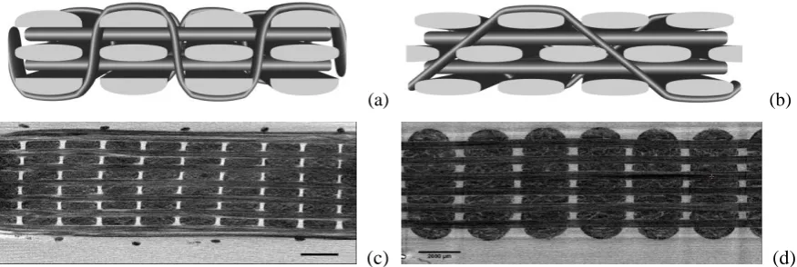
yarns. For the example of plain weave fabrics, each weft yarn crosses over a warp yarn, then under the next warp yarn, and so on. In a twill weave fabric, each weft yarn crosses over a number of warp yarns, u, then crosses under a number of warp yarns, b, thus forming a distinctive diagonal pattern. Hence, twill weave patterns are designated by a fraction, 𝑢/𝑏. Analytical prediction of the through-thickness permeability requires geometrical characterization of flow channels formed in the respective fabric structure. While X-ray micro-Computed Tomography (



were obtained using optical microscopy.

2 Theoretical analysis of

2.1 Orthogonal and angle-interlock woven fabrics

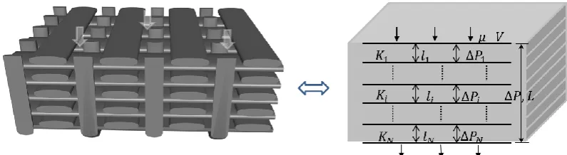
Here, a 3D woven fabric, either orthogonal or angle-interlock, is assumed to comprise a number of identical sub-layers. Each sub-layer is formed from one layer of warp yarns and one layer of weft yarns.. Since there is always one more weft layer than warp layer (Fig. 1a), the number of sub-layers is N+1/2. Since the ½ sub-layer only contains yarns aligned in one direction, the gap space is assumed to be large compared to a full (bi-directional) sub-layer, and its influence on the through-thickness permeability of the fabric is neglected. A homogenization approach [10, 17] _{was used to simplify the 3D woven structure, as}

shown in Fig. 2, where 𝑖 is an arbitrary sub-layer, while N is the total number of sub-layers. For laminar through-thickness flow of a Newtonian fluid through the fabric, the fluid is assumed to penetrate the sub-layers successively. According to Eq. 1, a linear relationship between ∆𝑃 𝐿⁄ and 𝑉 applies to an arbitrary sub-layer of the 3D woven fabric:

∆𝑃𝑖

𝑙𝑖 = −

𝜇

𝐾𝑖𝑉 (5)

The total pressure drop, ∆𝑃 = ∑𝑁𝑖=1∆𝑃𝑖, and thickness, 𝐿 = ∑𝑁𝑖=1𝑙𝑖, determine the value of 𝐾𝑧𝑧 of the 3D woven fabric based on Eq. 1:

∑𝑁 ∆𝑃_𝑖

𝑖=1 = −_𝐾𝜇𝑉_𝑧𝑧∑𝑁𝑖=1𝑙𝑖 (6)

Since the equation of continuity applies, thevalue of 𝑉 is identical for each fabric sub-layer. Thus,

∆𝑃 = ∑𝑁 ∆𝑃_𝑖

𝑖=1 = −𝜇𝑉 ∑ _𝐾𝑙𝑖

𝑖

𝑁

𝑖=1 (7)

4

𝐾𝑧𝑧= 𝐿

∑ 𝑙𝑖

𝐾𝑖 𝑁 𝑖=1

(8)

2.2 Sub-layer of 3D woven fabrics

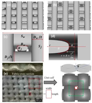
Unit cells of an orthogonal 3D woven fabric and a plain weave fabric are shown schematically in Fig. 3c and e. The through-thickness permeability, 𝐾𝑓, of a unit-cell depends on the yarn permeability, 𝐾𝑦, and equivalent permeability of inter-yarn gaps , 𝐾_𝑔. While 𝐾_𝑦 depends onfilament radius, 𝑅_𝑓, and yarn fibre volume fraction, 𝑉𝑓, [18-22] 𝐾𝑔 is determined by the in-plane gap dimensions and their change through the thickness.

In a fabric unit-cell, 𝑄𝑔 is the volumetric flow rate through the inter-yarn gap with cross-sectional area 𝐴𝑔; 𝑄𝑦 and 𝑄𝑓, and 𝐴𝑦 and 𝐴𝑓 are the corresponding parameters for yarns and the fabric. According

to Eq. 1, the relationship between 𝐾𝑦, 𝐾𝑔 and 𝐾𝑓is:

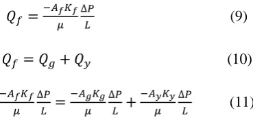
𝑄𝑓 =−𝐴_𝜇𝑓𝐾𝑓∆𝑃_𝐿 (9)

𝑄𝑓 = 𝑄𝑔+ 𝑄𝑦 (10)

−𝐴𝑓𝐾𝑓

𝜇 ∆𝑃

𝐿 =

−𝐴𝑔𝐾𝑔

𝜇 ∆𝑃

𝐿 +

−𝐴𝑦𝐾𝑦

𝜇 ∆𝑃

𝐿 (11)

If the area coverage in a fabric sub-layer is Ф = 𝐴𝑔⁄𝐴𝑓, Eq. 11 can be expressed as:

𝐾_𝑓= Ф𝐾_𝑔+ (1 − Ф)𝐾_𝑦 (12)

which describes the permeability for a sub-layer of a 3D woven fabric.

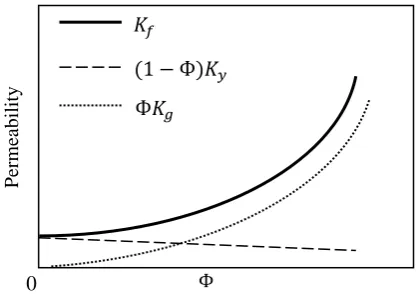
Figure 4 shows the fabric permeability and the contributions of equivalent gap permeability and yarn permeability as expressed in Eq. 12 as functions of Ф, assuming a constant value of 𝐾𝑦. If a fabric has a high yarn packing density, where inter-yarn gaps disappear ( = 0), 𝐾_𝑓 is equivalent to 𝐾_𝑦. As Ф increases, the contribution of 𝐾𝑦 to 𝐾𝑓 decreases linearly while 𝐾𝑔 increases significantly. A critical size of inter-yarn gap exists, where (1 - )Ky equals Kg, i.e. the two dashed curves in Fig. 4 cross, and

𝐾_𝑦 and 𝐾𝑔 contribute equally to 𝐾𝑓. The dependence of 𝐾𝑔 and 𝐾𝑦 on fabric geometrical parameters,

as indicated in Fig. 3c and d, will be discussed in the following.

Introducing some simplifications of the unit cell geometry (neglecting crimp if present, assuming straight warp and weft yarns with constant cross-section, assuming rectangular cross-section of the binder yarn), the actual gap cross-section (Fig. 3) can be characterized by the hydraulic radius [22-24]_:

𝑅 =

where 𝑆_𝑗, 𝐷_𝑗 and 𝐵_𝑗 are the measured spacing and width of warp yarns and height of binder yarns, while 𝑆_𝑤, 𝐷_𝑤 and 𝐵_𝑤 are the measured spacing and widths of weft yarns and width of binder yarns, respectively. While R is the hydraulic radius at the narrowest flow channel cross-section,

𝑎 = 𝑆𝑗𝑆𝑤

2(𝑆𝑗+𝑆𝑤)− 𝑅 (14)

is the distance from the narrowest flow channel boundary to the boundary of the unit-cell. A parabolic equation is used to approximate the yarn cross-section through-thickness with the coordinates in through-thickness direction, 𝑥, and in-plane, 𝑟, shown in Fig. 3d:

𝑟 = 𝑅 +𝑥2

𝜆𝑎 (15)

Here, the parameter, 𝜆, is related to the yarn height and determines the curvature of the channel geometry. The smaller the value of 𝜆, the sharper the tip of the yarn cross-section. The exact flow channel geometry can be obtained from microscopic images of cross-sections of warp and weft yarns, where coordinates can be measured using image analysis software and approximated by a second-order polynomial using least-squares analysis [22]_{. This allows the value of 𝜆 in Eq. 15 to be determined directly.}

Flow though a gap with varying cross-section is analysed based on the Hagen-Poiseuille equation [25]_,

assuming that at each position through-thickness the gap can be treated as a long straight tube:

∫ 𝑑𝑃𝑃1

𝑃2 =

8𝑐𝜇𝑄

𝜋 ∫

𝑑𝑥 (𝑅+𝑥2_𝜆𝑎)4 𝑙𝑖 2

−𝑙𝑖₂

(16)

Here c is a laminar friction constant for conversion of a duct with rectangular cross-section (with aspect ratio α=width/length) to a virtual circular duct with identical equivalent permeability, where



∆𝑃 =8𝑐𝜇𝑄 𝜋

√𝜆𝑎𝑅

𝑅4 {

5

8tan

−1₍ 𝑙𝑖

2√𝜆𝑎𝑅) +

𝑙𝑖

2√𝜆𝑎𝑅[15(𝑙𝑖 2 4𝜆𝑎𝑅)

2

+40𝑙𝑖_{4𝜆𝑎𝑅}2+33]

24(_{4𝜆𝑎𝑅}𝑙𝑖2 +1)3 } (17)

From Eqs. 1 and 17, 𝐾𝑔 can be obtained as follows:

𝐾_𝑔 = 𝑙𝑖∙𝑅2

8𝑐√𝜆𝑎𝑅∙

{

5

8tan−1(2√𝜆𝑎𝑅𝑙𝑖 )+ 𝑙𝑖 2√𝜆𝑎𝑅[15( 𝑙𝑖

6

If crimp is introduced, as in unit cells of 2D woven fabrics, determining 𝐾_𝑦 is more complicated because the yarn orientation relative to the flow direction varies for different weave architectures. While Gebart [18]

analyzed fluid flow along and perpendicular to parallel filaments with ideal periodic arrangement (i.e. in yarns), Advani et al. [26] _{summarized the theory of flow in anisotropic materials with an angle,} 𝜃_{, relative}

to the main flow direction. Combination of the two models gives an expression for 𝐾_𝑦 for undulated yarns with crimp angle, 𝜃, in a plain weave fabric:

𝐾𝑦1=8𝑅𝑓

2 53

(1−𝑉𝑓)3 𝑉_𝑓2 cos

2_{𝜃 +}16𝑅𝑓2 9√6𝜋(√

𝑉𝑓𝑚𝑎𝑥 𝑉𝑓 − 1)

5/2_sin2_{𝜃 −}

sin2_{𝜃 cos}2_𝜃(16𝑅𝑓2 9√6𝜋(√

𝑉𝑓𝑚𝑎𝑥 𝑉𝑓 −1)5/2−

8𝑅𝑓2 53

(1−𝑉𝑓)3 𝑉𝑓2 )2 8𝑅𝑓2

53 (1−𝑉𝑓)3

𝑉𝑓2 sin2𝜃+ 16𝑅𝑓2

9√6𝜋(√ 𝑉𝑓𝑚𝑎𝑥

𝑉𝑓 −1)5/2cos2𝜃

(19-1)

For a twill weave fabric characterized by 𝑢/𝑏, there are (𝑢 + 𝑏 − 1) (𝑢 + 𝑏)⁄ flat yarn segments and 1 (𝑢 + 𝑏)⁄ segments of yarns inclined at a crimp angle, 𝜃. Hence the total contribution of a yarn to the

through-thickness fabric permeability can be described as:

𝐾𝑦2=(𝑢+𝑏−1)_(𝑢+𝑏) ∙

16𝑅_𝑓2

9√6𝜋(√

𝑉_{𝑓𝑚𝑎𝑥}

𝑉𝑓

− 1

5 2

+

(𝑢+𝑏) (19-2)

Here, 𝑉𝑓 is the fibre volume fraction in a yarn; 𝑉𝑓𝑚𝑎𝑥 is the maximum fibre volume fraction, which is achieved when the filaments are in contact with each other. The value of Vfmax is π/4 for square filament arrangements and π 2√3⁄ for hexagonal filament arrangements [18]_{. The effect of low level yarn}

twist (Fig. 6a) on 𝐾𝑦 is ignored here. For unit cells of 3D woven fabrics as shown in Fig. 3c, 𝐾𝑦 is determined by fluid flow along filaments in binder yarns, and flow perpendicular to filaments in warp and weft yarns. Hence, from Gebart’s model and Eq. 11 for ratios of cross-sectional areas:

𝐾𝑦3=

𝑆𝑗∙𝑆𝑤−(𝑆𝑗−𝐷𝑗)∙(𝑆𝑤−𝐷𝑤)

𝑆𝑗∙𝑆𝑤 ∙

16𝑅𝑓2

9√6𝜋(√

𝑉𝑓𝑚𝑎𝑥

𝑉𝑓 − 1)

5 2

+𝐵𝑗∙𝐵𝑤

𝑆𝑗∙𝑆𝑤∙

8𝑅𝑓2

53

(1−𝑉𝑓)3

𝑉𝑓2 (20)

In Eqs. 19 and 20, yarn permeabilities are derived assuming hexagonal fibre arrangement. For a square fibre arrangement, the constants (53 and 9√6) would need to be replaced with 57 and 9√2.

3 Experimental study of

The equations for the permeabilities of sub-layers, 𝐾𝑓, and entire fabrics, 𝐾𝑧𝑧, were applied to four 3D woven carbon fibre reinforcement fabrics (two orthogonal and two angle-interlock fabrics) and validated based on experimental permeability data.

cross-section two layers of warp yarns and binder yarns, both with rectangular cross-section. Fabric ‘O’ is an orthogonal 3D woven fabric with six layers of warp yarns, seven layers weft yarns and binder yarns with approximately rectangular cross-section. The real internal geometry of the two 3D woven fabrics was characterized based on micrographs of composite specimens [11]_{. In Table 1,} 𝑁’ _{is the number of}

layers of 3D woven fabric, 𝑉_𝐹 is the fibre volume fraction in the fabric, i.e. the total fibre volume divided by the volume occupied by the fabric.

The through-thickness permeability was measured in a saturated uni-directional flow experiments. In a stiff cylindrical flow channel with a liquid inlet at the bottom and a liquid outlet on top (inner diameter 80 mm), fabric specimens are held in position by stiff perforated plates, which allow parallel flow perpendicular to the fabric plane. The distance between the perforated plates is given by the height of spacer rings. Engine oil with known viscosity-temperature characteristics (𝜇 ≈ 0.3Pa ∙ s at 20 ºC) was used as a test fluid. The flow rate is set on a gear pump and monitored using a flow meter. Pressure transducers are mounted on both sides of the fabric specimen for measurement of the pressure drop [11]_.

The value of 𝐾𝑧𝑧 was calculated according to Eq. 1 with the constant flow rate (laminar flow with small Reynolds numbers) and measured pressure drop. Each test was repeated three times with a fresh sample.

In addition, three 2D technical textiles (cotton or cotton/polyester) were analysed. Measured geometrical fabric parameters are listed in Table 2. Top view and side view images of 2D fabrics were acquired using an optical microscope. The images were used to measure the yarn spacing, 𝑆𝑥, from the distance between centrelines of two neighboring parallel yarns, yarn widths and heights, 𝐷𝑥 and 𝐵𝑥, from fabric cross sectional dimensions, and the values of 𝑅𝑓, 𝜆 and 𝑉𝑓. The fabric thickness, 𝐿, was tested using the Kawabata Evaluation System (KES-F) at an applied normal pressure of 0.05 kPa.

The through-thickness permeability of 2D fabrics was measured according to BS EN ISO 9237:1995. The apparatus for the experiment is an air permeability tester FX 3300. While the fabric is clamped in position, a suction fan forces air to flow perpendicularly through the fabric. The volumetric flow rate is measured and divided by the specimen area to give the velocity of air flow. The pressure drop in the experiment for all fabrics is set to 500 Pa, with an accuracy of at least 2 %. Using the measured velocity, pressure drop and fabric thickness, permeability is calculated according to Darcy’s law.

4 Results and discussions

8

either based on top or side views of the fabrics. The yarns in these 2D fabrics have ‘Z’- twist, which results in dense filament packing in the yarns and low values of 𝐾_𝑦. Since the level of yarn twist is low, Eq. 19 is suitable to approximate 𝐾𝑦 assuming aligned and parallel filaments.

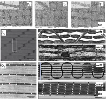
The cross-sections in Fig. 5b, illustrate the internal geometry of orthogonal and angle-interlock woven fabrics. The warp and weft yarns in the orthogonal 3D woven fabric are straight and parallel. Binder yarns follow paths through the fabric thickness, fixating warp and weft yarns and generating inter-yarn gaps to form flow channels. In the angle-interlock woven fabric, binder yarns follow paths resembling sine/cosine curves through the layers of warp and weft yarns. The cross-section normal to the weft direction shows an offset between layers of weft yarns by half a yarn width, which needs to be considered for definition of the angle-interlock fabric unit cell. The white rectangular frames in the top views of the fabrics illustrate the fabric unit cell areas. Measuring the geometrical dimensions of each fabric unit cell allows the sub-layer permeability, 𝐾𝑓, and the permeability of the entire fabric, 𝐾𝑧𝑧, to be predicted.

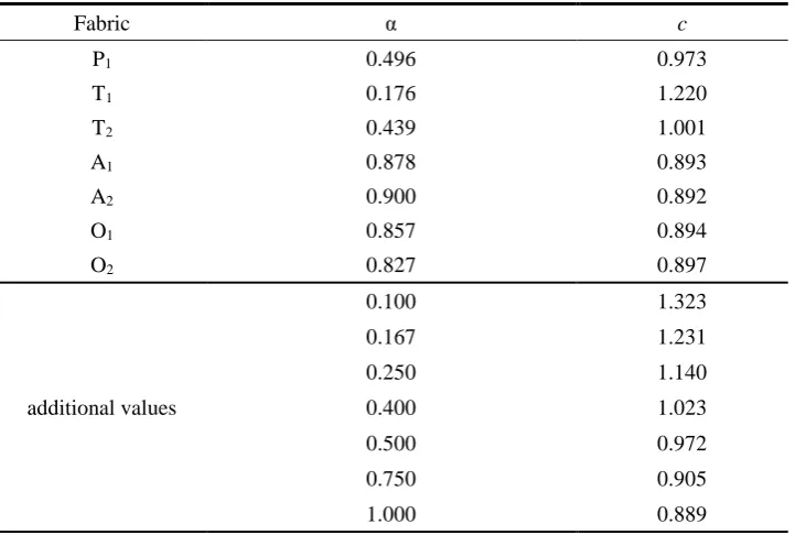
Table 3 gives measured values of α for the seven woven fabrics based on the measured yarn spacing and width in Tables 1 and 2. The value of c decreases with increasing value of α. Additional values for α are listed as reference for fabrics with different weave densities and porosities. Table 4 quantifies the contributions of 𝐾_𝑔 and 𝐾_𝑦 to 𝐾_𝑓 for 2D woven fabrics based on the measured dimensions and Eqs. 12, 18 and 19. The contribution of 𝐾𝑦 to 𝐾𝑓 is less than 12 % if Ф is greater than 1 %, indicating the significant effect of 𝐾𝑔 on 𝐾𝑓. For fabric P1, 𝐾𝑓 is greater than for fabrics T1 and T2, owing to the

greater value of Ф. Fabrics T1 and T2 show similar values of 𝐾_𝑓 since the values of Ф are similar. This

implies that for most 2D woven fabrics, 𝐾_𝑧𝑧 can be estimated merely considering 𝐾_𝑔 and Ф, and Eq. 19 only needs to be applied for fabrics with dense yarn packing. Figure 6 compares predicted(Eqs. 8 and 12) and measured values of 𝐾𝑧𝑧 for the seven woven fabrics. The comparison suggests that characterizing the internal structure of a fabric accurately and considering flow through an inter-yarn gap with varying cross-section (Fig. 3d) when determining the value of 𝐾_𝑔 (Eq. 18),, allows accurate prediction of 𝐾𝑓 for 2D fabrics or a sub-layer of a 3D woven fabric.

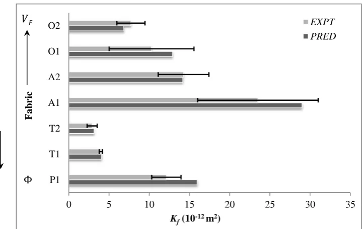
The predicted value of 𝐾𝑧𝑧 for orthogonal and angle-interlock 3D woven fabrics was based on Eqs. 8, 12, 18 and 20. The geometrical parameters and fabric specifications for the prediction were taken from Table 1. Fabric ‘A’ shows relatively wide gaps between adjacent parallel yarns and high 𝐾𝑧𝑧 values owing to the small values of 𝑉_𝐹 and high values of 𝐾_𝑖. For 𝑉_𝐹 = 0.41 (A1), the predicted value of 𝐾_𝑧𝑧, 28.9×10-12

m2_{, is similar to the measured average value, 23.5}×₁₀-12 _m2_{, indicating a relative difference of 23.3 %. For}

𝑉𝐹= 0.47 (A2), the prediction shows very good agreement with experimental data. Comparisons for fabric

‘O’ give similar result. For 𝑉𝐹 = 0.55 (O1), the measured 𝐾𝑧𝑧 is 10.3×10-12 m2whereas the prediction is

12.9×10-12 _m2_{. All predicted peremabilities for the 3D woven fabrics lie within the range defined by the}

increasing 𝑉_𝐹 due to the reduction of overall gap space in the fabric.

5 Conclusions

The though-thickness permeability of orthogonal and angle-interlock 3D woven fabrics was studied analytically. It is determined by the height and through-thickness permeability of each sub-layer, the number of sub-layers, and the entire fabric thickness. The through-thickness permeability of each sub-layer depends on the yarn permeability in the flow direction, the equivalent permeability of inter-yarn gaps and the areal coverage of the fabric. The yarn permeability was modeled by combining axial and transverse permeabilities based on the local yarn crimp angle. The equivalent gap permeability was modelled based on conversion of the actual gap cross-section to a circular cross-section and varying the cross-section through the fabric thickness according to measured yarn cross-sectional profiles. For seven woven fabrics of different architectures, geometrical fabric parameters were characterized in detail by optical microscopy. Calculation of yarn permeability, equivalent gap permeability, and fabric permeability shows that the equivalent gap permeability dominates the fabric permeability, even if the areal coverage of inter-yarn gaps is only around 1 %. Comparison of predicted and measured values of the through-thickness permeability of orthogonal and angle-interlock woven fabrics shows close agreement for each sample, indicating good accuracy of the permeability models. Studies on the sensitivity of the fabric through-thickness permeability to variation of the geometrical parameters and extension of the theoretical analysis to 3D woven fabrics with different architecture are ongoing.

Acknowledgements

The work was supported in part by the projects: RGC No.: 5158/13E and NSFC funding Grant No. 51373147 and Project code: JC201104210132A.

Appendix

The frictional pressure loss in flow along a duct with arbitrary cross section, e.g., the duct formed by interwoven yarns, is usually expressed in terms of a friction factor ξ (also called a resistance coefficient) which is defined as [27]_:

ξ =∆P L ∙

2Dh

ρV2 (a1)

10

𝐷_ℎ= 4𝐴′ 𝑂⁄ (a2)

For a circular tube, 𝐷ℎ is equivalent to its geometrical diameter. The friction factor can be derived analytically for many cross sections (circular, triangular, quadratic, etc.) in laminar flows [18,28] _{and can be}

expressed as:

ξ = c′ ∙_𝜌𝑉𝐷𝜇

ℎ (a3)

where c’ is a dimensionless shape factor and



∆𝑃 𝐿 = 𝑐′ ∙

𝜇𝑉

2𝐷ℎ2 (a4)

Comparing Eq. 1 with Eq. a4 gives:

K =2𝐷ℎ2

𝑐′ (a5)

The Hagen–Poiseuille equation describes a laminar fluid flow along a circular tube (diameter 𝐷ℎ), which has a relationship of pressure gradient and flow velocity:

∆𝑃

𝐿 =

32𝜇𝑉

𝐷ℎ2 (a6)

Comparison of Eqs. a6 and 1 gives the equivalent permeability of a circular tube:

K_𝑡 =𝐷ℎ2

32 (a7)

This implies that the valueof c’ is 64.

When converting ducts with arbitrary rectangular cross-section to virtual ducts with circular cross-section, friction constants reported in the literature [29] _{for rectangular ducts with different width/length ratio, α,}

were divided by c’ to obtain c as listed in Table 3. These values can be fitted with a polynomial (coefficient of correlation R2_=1):

𝑐 = 1.5 − 2.0364𝛼 + 2.964𝛼2_{− 2.724𝛼}3_{+ 1.677𝛼}4_{− 0.491𝛼}5 _(a8)

According to Eq. a8, the value of c can be obtained for calculation of 𝐾𝑔 for arbitrary gap length and width ratios, as demonstrated for the seven fabrics in Table 3.

References

[1] Mallick PK. Fiber-reinforced composites: materials, manufacturing, and design. Third Edition, Taylor & Francis

Group, 2007.

Netherlands, 1999.

[3] Long A. Design and manufacture of textile composites. Woodhead Publishing Limited, Cambridge, UK, 2005.

[4] Greene DL. Energy-efficiency improvement potential of commercial aircraft. Annual Review of Energy and

Environment, 1992, 17: 537-573.

[5] Zeng X, Brown LP, Endruweit A, Matveev M, Long AC. Geometrical modelling of 3D woven reinforcements

for polymer composites: Prediction of fabric permeability and composite mechanical properties. Composites Part A:

Applied Science and Manufacturing, 2014, 56, 150-160.

[6] Hickey CMD, Bickerton S. Cure kinetics and rheology characterization and modelling of ambient temperature

curing epoxy resins for resin infusion/VARTM and wet layup application. Journal of Materials Science, 2013, 48(2):

690-701.

[7] Endruweit A, Glover P, Head K, Long AC. Mapping of the fluid distribution in impregnated reinforcement

textiles using Magnetic Resonance Imaging: application and discussion. Composites. Part A: Applied Science and

Manufacturing, 2011, 42(10), 1369-1379.

[8] Grujicic M, Chittajallu KM, Shawn W. Lattice Boltzmann method based computation of the permeability of the

orthogonal plain-weave fabric preforms. Journal of Materials Science, 2006, 41(23): 7989-8000.

[9] Mei CC, Vernescu B. Homogenization methods for multiscale mechanics, 2010: Singapore; London; World

Scientific. 330.

[10] Mogavero J, Advani SG. Experimental investigation of flow through multi-layered preforms. Polymer

Composites, 1997, 18(5): 649-655.

[11] Endruweit A, Long AC. Analysis of compressibility and permeability of selected 3D woven reinforcements.

Journal of Composite Materials, 2010, 44(24): 2833-2862.

[12] Desplentere F, Lomov SV, Woerdeman DL, Verpoest I, Wevers M and Bogdanovich A. Micro-CT

characterization of variability in 3D textile architecture. Composites Science and Technology, 2005, 65(13):

1920-1930.

[13] Badel P, Vidal-Salle E, Maire E and Boisse P. Simulation and tomography analysis of textile composite

reinforcement deformation at the mesoscopic scale. Composites Science and Technology, 2008, 68(12): 2433-2440.

[14] Mahadik Y, Brown KAR and Hallett SR. Characterization of 3D woven composite internal architecture and

effect of compaction. Composites Part A-Applied Science and Manufacturing, 2010, 41(7): 872-880.

[15] Awal A, Ghosh SB, Sain M. Development and morphological characterization of wood pulp reinforced

biocomposite fibers. Journal of Materials Science, 2009, 44(11): 2876-2881.

[16] Karahan M, Lomov SV, Bogdanovich AE, Mungalov D, Verpoest I. Internal geometry evaluation of non-crimp

3D orthogonal woven carbon fabric composite. Composites Part A: Applied Science and Manufacturing, 2010,

41(9): 1301-1311.

[17] Rocha RPA, Cruz ME. Calculation of the permeability and apparent permeability of three-dimensional porous

media. Transport in Porous Media, 2010, 83(2): 349-373.

12

26(8): 1101-1133.

[19] Cai Z, Berdichevesky AL. An improved self-consistent method for estimating the permeability of a fiber

assembly. Polymer Composites, 1993, 14(4): 314-323.

[20] Bruschke MV, Advani SG. Flow of generalized Newtonian fluids across a periodic array of cylinders. Journal

of Rheology, 1993, 37(3): 479-497.

[21] Xiao X, Long A, Zeng X. Through-thickness permeability modelling of woven fabric under out-of-plane

deformation. Journal of Materials Science, 2014, 49: 7563-7574.

[22] Xiao X, Zeng X, Long AC, Cliford MJ, Lin H, Saldaeva E. An analytical model for through-thickness

permeability of woven fabric. Textile Research Journal, 2012, 82(5): 492-501.

[23] Zupin Z, Hladnik A and Dimitrovski K. Prediction of one-layer woven fabrics air permeability using porosity

parameters. Textile Research Journal, 2012, 82(2): 117-128.

[24] Mehaute B. An introduction to hydrodynamics & water waves. Springer-Verlag, New York, 1976.

[25] Sutera, SP, Skalak R. The history of Poiseuille's law. Annual Review of Fluid Mechanics, 1993. 25: 1-19.

[26] Advani SG, Bruschke MV, Parnas RS. Resin transfer molding flow phenomena in polymeric composites, In ‘Flow and rheology in polymer composites manufacturing’. Elsevier science B. V, Amsterdam, 1994.

[27] Schlichting H., Gersten K. Boundary-Layer Theory. 8th _{Edition, Birlin, Hong Kong, Springer, c2000.}

[28] Batchelor G.K. An introduction to fluid dynamics. Cambridge, Cambridge University Press, c1967.

[29] Papautsky I., Gale B.K., Mohanty S., Ameel T.A., Frazier A.B. Effects of rectangular microchannel aspect ratio

on laminar friction constant. Proceedings of the Society of Photo-Optical Instrumentation Engineers (SPIE), 1999,

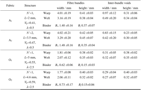
Table 1 Geometrical fabric parameters for four 3D woven carbon fibre fabrics

Fabric Structure Fibre bundles Inter-bundle voids

width / mm height / mm width / mm height / mm

A1

N’=1,

L=2 mm,

𝑉𝐹=0.41,

𝜆=0.5

Warp 4.01 ±0.19 0.41 ±0.03 0.97 ±0.12 0.31 ±0.06

Weft 3.16 ±0.19 0.38 ±0.04 0.49 ±0.20 0.34 ±0.04

Binder Bw 1.40 ±0.16 Bj 0.37 ±0.07

A2

N’=2,

L=3.5 mm,

𝑉𝐹=0.47,

𝜆=0.5

Warp 4.02 ±0.21 0.42 ±0.05 0.83 ±0.15 0.23 ±0.05

Weft 3.29 ±0.20 0.45 ±0.07 0.42 ±0.20 0.30 ±0.05

Binder Bw 1.48 ±0.16 Bj 0.35 ±0.04

O1

N’=1,

L=5 mm,

𝑉𝐹=0.55,

𝜆=2.5

Warp 1.81 ±0.06 0.38 ±0.02 0.31 ±0.05 0.38 ±0.02

Weft 2.07 ±0.12 0.35 ±0.03 0.32 ±0.07 0.35 ±0.03

Binder Bw 0.62 ±0.06 Bj 0.15 ±0.03

O2

N’=1,

L=4.6 mm,

𝑉𝐹=0.59,

𝜆=2.5

Warp 1.77 ±0.08 0.40 ±0.03 0.29 ±0.04 0.40 ±0.03

Weft 2.06 ±0.11 0.32 ±0.02 0.27 ±0.07 0.32 ±0.07

Binder Bw 0.73 ±0.17 Bj 0.15±0.06

Table 2 Geometrical fabric parameters for three 2D woven fabrics

Fabric Structure 𝑅𝑓 /

m

Yarn

𝑉𝑓

𝐿 / mm 𝜆 /

mm-1

Yarn spacing Yarn width

Sj /

mm

Sw /

mm

Dj /

mm

Dw /

mm

P1

plain

(100 % cotton) 4.3 0.56 0.323 5.23 0.470 0.410 0.405 0.279

T1

2/1 twill

(67 %

polyester,

33 % cotton)

5.9 0.56 0.419 3.81 0.340 0.480 0.310 0.310

T2

2/2 twill (60 %

cotton, 40 %

polyester)

14

Table 3 Aspect ratios, , of rectangular gaps (width/length) and corresponding values of conversion friction factor, c

Fabric α c

P1 0.496 0.973

T1 0.176 1.220

T2 0.439 1.001

A1 0.878 0.893

A2 0.900 0.892

O1 0.857 0.894

O2 0.827 0.897

additional values

0.100 1.323

0.167 1.231

0.250 1.140

0.400 1.023

0.500 0.972

0.750 0.905

1.000 0.889

Table 4 Comparison of the predicted yarn and inter-yarn gap permeabilities for 2D woven fabrics

Fabric Ф 𝐾𝑦 / 10-13 m2 𝐾𝑔 / 10-10 m2 𝐾𝑓 / 10-12 m2 (100 % − Ф)𝐾𝑦/𝐾𝑓 Ф𝐾𝑔/𝐾𝑓

P1 3.93 % 3.00 3.99 15.97 1.80 % 98.20 %

T1 1.64 % 4.98 2.19 4.08 12.01 % 87.99 %

(a) (b)

(c) (d)

Fig. 1 Cross-sections of 3D woven fabrics; geometrical models of orthogonal (a) and angle-interlock (b) fabrics,

normal to weft direction; -CT scans [5] _{of an orthogonal fabric, normal to warp direction (c) and normal to weft}

16

Fig. 3 Top view of orthogonal (a) andangle-interlock (b) fabrics; top view of a unit-cell of orthogonal weave (c) and

side view normal to warp direction (d) with dimensions; (e) left: top and side views of a plain weave fabric; (e) right:

fabric unit-cell where the red frame indicates the inter-yarn gap, and the green frame indicates the yarn area;, 𝜃 is

18

Fig. 4 Schematic of relationship of three permeabilities, 𝐾𝑦, 𝐾𝑔 and 𝐾𝑓.

Φ

Per

m

ea

b

ilit

y

𝐾𝑓

(1 − Ф)𝐾𝑦

Ф𝐾𝑔

Fig. 5 (a) Top views and cross-sections of woven fabrics P1, T1, T2; (b) top views and cross-sections normal to warp

and weft directions of fabrics A1 and O1

(a)

20

Fig. 6 Predicted fabric permeabilities (Eqs. 8, 12, 18 & 20) compared to experimental data; error bars indicate

standard deviations.

0 5 10 15 20 25 30 35

P1 T1 T2 A1 A2 O1 O2

K_f(10-12 _m2₎

F

a

bric

EXPT PRED