Fiscal policy and learning

C

D

M

A

W

P

S

*We are very grateful for financial support from ESRC Grant RES-062-23-2617 and from National Science Foundation Grant no. SES-1025011 without which this work could not have been carried out. Any views expressed are those of the authors and do not necessarily reflect the views of the Bank of Finland. Corresponding author: Kaushik Mitra, School of Economics & Finance, University of St Andrews, Castlecliffe, The Scores, St Andrews, Fife, KY16 9AL, UK. Phone: + 44 (0) 1334 461951, Fax: 44 (0) 1334 462444, Email:

[email protected].

CASTLECLIFFE,SCHOOL OF ECONOMICS &FINANCE,UNIVERSITY OF ST ANDREWS,KY169AL

TEL:+44(0)1334462445 FAX:+44(0)1334462444 EMAIL:[email protected]

CDMA12/02

*

Kaushik Mitra

University of St Andrews

University of Oregon and

George W. Evans

University of St Andrews

Seppo Honkapohja

Bank of Finland

JANUARY

17,

2012

A

Using the standard real business cycle model with lump-sum taxes, we analyze the impact of fiscal policy when agents form expectations using adaptive learning rather than rational expectations (RE). The output multipliers for government purchases are significantly higher under learning, and fall within empirical bounds reported in the literature (in sharp contrast to the implausibly low values under RE). Effectiveness of fiscal policy is demonstrated during times of economic stress like the recent Great Recession. Finally it is shown how learning can lead to dynamics empirically documented during episodes of “fiscal consolidations.”

JEL Classification:E62, D84, E21, E43.

Keywords:Government Purchases, Expectations, Output Multiplier, Fiscal

1

Introduction

There has been a recent revival of interest in the eectiveness ofscal policy in the wake of policy measures enacted by governments all over the world to combat the damaging eects of the “Great Recession”.1 _{Of course, interest}

inscal policy is not a recent phenomenon; there were several studies in the 1980s and 90s examining their eects as in Barro and King (1984), Baxter and King (1993), Aiyagari, Christiano, and Eichenbaum (1992). However, with the advent of in ation targeting as a framework for monetary policy adopted by leading central banks over the world, attention shifted to the development of suitable monetary policies for low in ation and stable growth. The eects from the subprime crisis in August 2007 and more dramatically the collapse of Lehman Brothers in September 2008 shattered belief in the “Great Moderation” achieved since the late 1980s. With interest rates close to zero and monetary policy seemingly proving ineective to tackle the eects of the Great Recession, governments naturally turned their attention toscal measures to combat the severe recessionary impacts on the economy.

These measures in turn have led to renewed interest in scal policy and a fairly voluminous recent literature; see for instance Hall (2009), Barro and Redlick (2011), Ramey (2011b), Ramey (2011a), Leeper, Traum, and Walker (2011), and Coenen, Erceg, Freedman, Furceri, Kumhof, Lalonde, Laxton, Linde, Mourougane, Muir, Mursula, Resende, Roberts, Roeger, Snudden, Trabandt, and Veld (2012). One thread running through this literature is measuring the eectiveness of scal policy through examinations of govern-ment purchases multipliers in the context of exogenous changes in defense spending. An example often used in these studies is that of a war that leads to temporary increases in military expenditures. This interpretation is mod-eled by a surprise temporary increase in government purchases as emphasized in the earlier studies of Barro and King (1984), and Baxter and King (1993). A common perception in the literature is that the standard neoclassical (Real Business Cycle aka RBC) model is an inadequate model for the study of this particular policy experiment. It is argued that the basic mechanism through which a temporary increase in government purchases works its way in the RBC model leads to the inescapable conclusion of very low output multipliers that are well outside the range found in empirical studies; see,

1_{Among activescal strategies adopted in the US and UK include temporary tax cuts}

in particular, the forceful arguments on this point made by Hall (2009), p. 185. The conclusion is that Keynesian or New Keynesian models with an aggregate demand channel are needed to deliver sizable government spending multipliers.

The recent analyses are almost invariably developed under the “rational expectations” (RE) hypothesis. While not denying the potential importance of aggregate demand channels of changes in government spending, a ques-tion of considerable interest is the extent to which the generally small size of multipliers in the RBC model depends on RE. This question is of im-portance regardless on one’s views concerning the role of aggregate demand channels, since most modern dynamic macroeconomic general equilibrium models incorporate the neoclassical mechanisms that are central to the RBC model.2

Thus, in the current paper we study t he impact of government purchases in the standard RBC model with the sole modication that we replace RE with agents who have incomplete information about the eects of policy changes and are learning adaptively over time about these changes.3 _{As we}

have argued in Evans, Honkapohja, and Mitra (2009) and in Mitra, Evans, and Honkapohja (2011), the assumption of RE is very strong and unreal-istic when analyzing policy changes. Economic agents need to have com-plete knowledge of the underlying structure, both before and after the policy change. They must also rationally and fully incorporate this knowledge in their decision making, and do so under the assumption that other agents are equally knowledgeable and equally rational. Our approach, in contrast, uses an adaptive learning model in which agents have partial structural knowl-edge. At each date agents’ consumption and labor supply choices depend on the time path of expected future wages, interest rates and taxes. In line with the standard literature of adaptive learning, we assume that agents’ forecasts of wages and interest rates are based on a statistical model, with coe!cients updated over time using least-squares. However, for forecasting future taxes agents use the path of future taxes under the assumption that

2_{For example, Leeper, Traum, and Walker (2011) report simulated multipliers for a}

series of nested models in which the New Keynesian models are specied as generalizations of the RBC model.

3_{For discussion of the adaptive learning approach and extensive references, see, for}

this is announced credibly by policymakers.

This approach seems very natural to us. The essence of the adaptive learning approach is that agents do not understand the general equilibrium considerations that govern the evolution of the central endogenous variables, i.e. aggregate capital, aggregate labor and factor prices, and are therefore assumed to forecast these variables statistically. On the other hand, agents can be expected to immediately incorporate into their decisions the direct implications of credible announcements of the paths of future taxes on their future net incomes. Once we allow for adaptive learning in this fashion it turns out that output multipliers for a temporary change in government purchases are much higher for the standard RBC model than under RE, and indeed are in line with the range provided by the empirical literature.

Using this approach, the eectiveness of scal policy undertaken during times of economic stress (as during the Great Recession) is analyzed next. We model a scenario designed to capture important features ofscal policy changes by governments to combat the Great Recession. Wend that output multipliers of changes in government purchases continue to be high under adaptive learning in contrast to the values found under RE. This suggests thatscal policy can be an eective stabilization tool in deep recessions. We note that we are able to obtain these results within the standard RBC model without the need to add any other frictions to the setup.

As a nal contribution we use the RBC model with learning to consider the episodes of so-called “expansionaryscal consolidations” that have been widely studied since the seminal contribution of Giavazzi and Pagano (1990). It is known that the RBC model under RE is unable to deliver dynamics of consumption, and especially investment, that are consistent with the em-pirical evidence during these scal episodes. However, the introduction of adaptive learning leads to behavior of these variables which is consistent with the evidence during these episodes. Thus, we are able to provide a sim-ple theory that can explain the major features during these episodes without the need for “special theories” for large versus small changes in scal pol-icy. The need for simple theories to explain these episodes has been strongly argued in Alesina, Ardagna, Perotti, and Schiantarelli (2002).

Section 6 describes how the introduction of learning in the RBC model can give a better match to features of data observed during the “expansionary

scal consolidations.” The nal section concludes.

2

The Model

There is a representative household who has preferences over non-negative streams of a single consumption goodfw and leisure 1qw given by

ˆ

Hw{

" X

v=w

v3wX(fv>1qv)}> where X(fv>1qv) = lnfv+ln(1qv) (1)

HereHˆw denotes potentially subjective expectations at time w for the future, which agents hold in the absence of rational expectations. The analysis of the model under RE is standard. When RE is assumed we indicate this by writingHw forHˆw. Our presentation of the model is general in the sense that it applies under learning as well as under RE. The form of the utility function in (1) has been used frequently, e.g. Long and Plosser (1983).4

The household ow budget constraint is

dw+1 = zwqw+uwdwfwk>w> where (2)

uw = 1+un>w= (3)

Here dw is per capita household wealth at the beginning of time w, which equals holdings of capitalnwowned by the household less their debt (to other households), esw> i.e. dw nw esw= uw is the gross interest rate for loans made to other households,zw is the wage rate,fw is consumption,qw is labor supply andk>w is per capita lump sum taxes. Equation (3) arises due to the absence of arbitrage from loans and capital being perfect substitutes as stores of value;un>wis the rental rate on capital goods, andis the depreciation rate. Households maximize utility (1) subject to the budget constraint (2) which yields the Euler equation for consumption

f3_w1 =Hˆwuw+1f3w+11 = (4)

4_{King, Plosser, and Rebello (1988), emphasize that log utility for consumption is needed}

From the ow budget constraint (2) we can get the intertemporal budget constraint (in realized terms) assuming the relevant transversality condition holds:

0 = uwdw+ " X

m=1

(Gw>w+m(w))31"w+m +"w> (5)

where Gw>w+m = m Q l=1

uw+l, m 1 and"wzwqwfwk>w>

Note that (5) involves future choices of labor supply by the household which can be eliminated to derive the linearized consumption function. For this we make use of the static householdrst order condition

(1qw)31 =zwf3w1=

This relationship can be used to substitute out qw+m in (5) and we can then obtain an expected value intertemporal budget constraint

0 =uwdw+"w+

" X

m=1 ˆ

Hw(Gw>w+m)31{zw+m (1 +)fw+mk>w+m}=

To obtain its optimal choice of consumptionfw, the household is assumed to use a consumption function based on a linearization around steady state values. In particular, we assume agents linearize the expected value intertem-poral budget constraint and the Euler equation around the initial steady state values¯f>d>¯ z>¯ ¯k andu¯=31. This linearization point is natural since agents can be assumed to have estimated precisely the steady state values before the policy change that takes place.

As shown in Mitra, Evans, and Honkapohja (2011), substituting the lin-earized Euler equation (4) into the intertemporal budget constraint, one ob-tains the consumption function

(fw¯f)

(1 +)

(1) = ¯d(uw¯u) +

31

(dw¯d)(k>w¯k)

where

Vu_wh

" X

m=1

m+1

m X

l=1

(uh_w+lu¯)> (7)

Vhk>w " X

m=1

m(hk>w+m¯k)> (8)

Vz_wh

" X

m=1

m(z_wh_+mz¯)> (9)

denote “present value” type expressions.

Equation (6) species a behavioral rule for the household’s choice of cur-rent consumption based on pre-determined values of initial assets, real in-terest rates, wage rates, current values of lump-sum taxes and (subjective) expectations of future values of wages, interest rates, and lump-sum taxes. Expectations are assumed to be formed at the beginning of period w and, for simplicity, we assume these to be identical across agents (though agents themselves do not know this to be the case). Equation (6) can then be viewed as the behavioral rule for per capita consumption in the economy.

To implement its behavioral rule, the household requires forecasts for

uh

w+l> zhw+m> and hk>w+m= For taxes hk>w+m (and ¯k) we assume that agents use

“structural” knowledge based on announced government spending rules. For convenience, we assume balanced budgets, so that k>w+m = jw+m. For uhw+l andzh

w+m we assume that household estimate future values using a VAR-type model in nw> zw> un>w and yw, with coe!cients updated over time by recursive least squares (RLS). The detailed procedure is described below in Section 3. To complete the model, we describe the evolution of the other state vari-ables, namelyzw> un>w> uw> |w andnw+1. Households own capital and labor

ser-vices which they rent torms. Therm uses these inputs to produce output

|w using the Cobb-Douglas production technology

|w =ywnwq

13 w >

whereyw is the technology shock that follows an AR(1) process

ˆ

yw=yˆw31+ ˜xw (10)

withyˆw= (ywy¯)=Here¯yis the mean of the process andx˜wis an iid zero-mean process following a normal distribution with constant variance2

Prot maximization by rms implies the standard rst-order conditions involving wages and rental rates

zw = (1)yw(

nw qw

) andun>w=yw( qw nw

)13=

In equilibrium, aggregate private debteswis zero, so thatdw =nw>and market clearing determinesnw+1 from

nw+1 =ywnwqw13+ (1)nwfwjw>

wherejw is per capita government spending.

For simulations of the model we follow standard procedures and approx-imate the path using a linearization around the steady state values. To analyze the impact of policy in the model, we compare the dynamics under learning to those under RE. At this stage we remark that, as is well known, under RE and in the absence of a policy change the endogenous variables,

nw+1> fw> qw> zw> un>w> uwcan be written as an (approximate) linear function ofnw

and yw, e.g. Campbell (1994). The RE solution can be written in the form of a stationary VAR(1), in the state{ˆ0w

³

ˆ

nw>yˆw ´

,

μ _ˆ

nw+1 ˆ

yw+1

¶ =E μ _ˆ nw ˆ yw ¶ + μ 0 1 ¶ ˜

xw+1> where E =

μ

2 iny

0 ¶

> (11)

with the other variables given by linear combinations of the state; the hatted values are deviations from the RE deterministic steady state i.e. nˆw =nw¯n etc. Note also that under RE forecasts of futurezˆw+m andˆun>w+m are given by linear combinations of the forecasted future state{ˆhw+m =Em{ˆw.

The focus of this paper is on policy changes. The method for obtaining the impact of policy changes under RE is standard, e.g. see Ljungqvist and Sargent (2004), Ch. 11 or Mitra, Evans, and Honkapohja (2011) for the details. We now turn to obtaining the dynamics under learning when there is a policy change.

3

Learning dynamics

rates, since these are required in order for agents to solve for their optimal level of consumption. We continue to follow this approach with respect to interest rates and wage rates, but for forecasting taxes agents are assumed to understand the future course of taxes implied by the announced policy. Agents in eect are given structural knowledge of the scal implications of the announced change in government purchases.5

As argued in the Introduction, we think this is a natural way to proceed, since changes in agents’ own future taxes have a quantiable direct eect, while future wages and interest rates are determined through dynamic gen-eral equilibrium eects. According to the adaptive learning perspective it is unrealistic to assume that agents understand the economic structure su! -ciently well to improve on reduced form econometric forecasts of aggregate variables like wages and interest rates. Thus we assume that when a policy change is announced, agents calculateVh

k>wusing the announced changes. To keep things simple, we assume that the government operates and is known to operate under a balanced-budget rule. The assumption of balanced budget with lump-sum taxes is often the maintained assumption in the cited works in the Introduction for analyzing the eects of changes in government pur-chases on output. Additionally, with lump-sum taxes, exogenous spending and appropriate additional assumptions, Ricardian Equivalence holds under both RE and learning, so that our results hold more generally; see e.g. Evans, Honkapohja, and Mitra (2011).

The rst policy change we examine in Section 4 is that of a temporary increase in (per capita) government purchases, j from j¯ to j¯0 for Wj 1 periods, announced to take place immediately at w= 1, i.e.

jw=w =

½

¯

j0_{, w = 1> ===> W}

j1

¯

j,w Wj> (12)

i.e., government purchases and taxes are changed in period w = 1 and this change is reversed at a later periodWj (this is often termed asurprise change inj in the literature). In our example in Section 4 we setWj = 9quarters so that we are considering a two-year increase inj.

Given their structural knowledge of the government budget constraint and the announced path of government purchases, the agents can thus compute

5_{A related approach is followed in Preston (2006) and Eusepi and Preston (2010) in}

the present value of the increase in their future taxes as

Vh_k>w =

" X

m=1

m(jw+mj¯) =

½

13(¯j0j¯)(1

Wj3w31_),1

wWj2

0> for wWj1=

Under learning, agents also need to form forecasts of future wages and inter-est rates since these are needed for their individual consumption choice in (6). Moreover, they need to form forecasts of these variables without full knowl-edge of the underlying model parameters. Wage and interest rate forecasts under learning depend on the perceived laws of motion (PLMs) of agents, with parameters updated over time in response to the data. We consider PLMs where future capital, wages, and rental rates depend on the current capital stock and technological shock,nw andyw. That is, we consider PLMs of the form

nw+1 = en+dnnnw+dnyyˆw+qrlvh> (13)

zw = ez +dznnw+dzyˆyw+qrlvh> (14)

un>w = eu+dunnw+duyˆyw+qrlvh> (15)

ˆ

yw = yˆw31+ ˜xw= (16)

where the PLM parameters en> dnn> dny etc. will be estimated on the basis of actual data. The nal line is the stochastic process for evolution of the (de-meaned) technological shock, which for simplicity is assumed known to the agents. In real-time learning, the parameters in (13), (14), (15) are time-dependent and are updated using RLS; see for e.g. Evans and Honkapohja (2001) p. 233. We also assume agents allow for structural change, which includes policy changes as well as other potential structural breaks, by dis-counting older data as discussed below.

Under RE, in contrast to learning, agents are assumed to know all of the underlying parameters involved in the REE solution, i.e. the parameters in (11), (13), (14), and (15) which they use to form future forecasts of wages and rental rates. The learning perspective is that assuming such knowledge is implausibly strong and hence unrealistic.

In particular, previousscal policy changes (if any), of the type considered in this paper, are likely to have varied in terms of the magnitude and duration of the change in government spending, and the state of the economy in which it was announced and implemented. Since older information of this type would probably have limited value, we assume that agents respond to policy change by updating the parameters of the PLM (13) - (15) as new data become available.6

Before discussing how the PLM coe!cients are updated over time using least-squares learning, we describe how (13) - (15) are used by agents to make forecasts. Given coe!cient estimates and the observed state (nw>yˆw), equa-tions (13) and (16) can be iterated forward to obtain forecastsnh

w+m and yˆw+m

form = 1>2> = = = = Wage and rental rate forecastszwh+m> un>wh +m are then obtained

using the relationships (14) - (15) while interest-rate forecasts are given by

uh

w+m = 1+un>wh +m. Given these forecasts,Vzwh andVuhw are computed from (9) and (7), which in turn are used in (6) in determining consumption in the temporary equilibrium. See the Appendix of Mitra, Evans, and Honkapohja (2011) for further details.

Parameter updating by agents using RLS learning is as follows. We dene the timew parameter estimates as

!_n>w =

3 C denn>wn>w

dny>w

4

D> !_z>w=

3 C dezn>wz>w

dzy>w

4

D> !_un>w =

3 C deun>wu>w

duy>w

4 D> }w=

3

C n1w

ˆ

yw

4

D=

The RLS formulas corresponding to estimates of equation (13), (14), and (15) are

!n>w = !n>w31+U3 1

w }w31(nw!0n>w31}w31)>

!_z>w = !_z>w31+U_w31}w31(zw31!0z>w31}w31)>

!_un>w = !_un>w31+U3_w1}w31(un>w31!0un>w31}w31)=

Uw = Uw31+(}w31}w031Uw31)=

The gain is assumed to be the same in all of the regressions for simplicity and is not essential. The initial values of all parameter estimates ! and U

are set to the initial steady state values under RE.

6_{See Evans, Honkapohja, and Mitra (2009) for an example of learning from repeated}

Here it is assumed that agents update parameter estimates using “dis-counted least squares,” i.e. they discount past data geometrically at rate

1, where 0 ? ? 1 is typically a small positive number. In the learn-ing literature the parameter is known as the “gain,” and discounted least squares is also called “constant-gain” least squares.

Constant-gain least squares is widely used in the adaptive learning lit-erature because it weights recent data more heavily. For a sample see, for example, Sargent (1999), Orphanides and Williams (2007), Carceles-Poveda and Giannitsarou (2008), and Eusepi and Preston (2011). In the current con-text constant gain is particularly appealing since agents will be aware that policy changes will induce changes in forecast-rule parameter values taking a possibly complex and time-varying form. The use of a constant-gain rule al-lows parameter estimates to track changes in parameter values more quickly than does “decreasing-gain” least squares.

4

Multipliers for Government Purchases

is 20% and that of consumption/output ratio is 59%= x˜w is assumed to be distributed normally with zero mean and standard deviation x = 0=007, which is in line with the value used in this literature.

Our choice of the gain parameter = 0=04 is in line with most of the literature, e.g. Branch and Evans (2006), Orphanides and Williams (2007), and Milani (2007). Eusepi and Preston (2011) use a much smaller value for the gain, but they do not consider changes in policy, for which a larger value of is more appropriate.

For the policy exercises, there is an increase in government purchases from

¯

j = 0=20to¯j0 _{= 0=21(a5%increase) that takes place atw = 1, and lasts until}

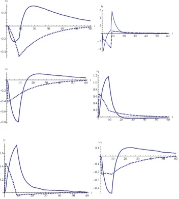
Wj = 9, i.e. for eight quarters (e.g. a two-year war) in equation (12). We plot the mean time paths for each endogenous variable over100>000 replications in Figure 1.

Under RE the dynamics are well understood, see Baxter and King (1993) and Mitra, Evans, and Honkapohja (2011) for details. nw falls as long as the policy change is in eect and then increases towards the (unchanged) steady state. fwfalls on impact and then increases monotonically towards the steady state. An important feature of a temporary increase inj is that consumption smoothing by agents is achieved by areduction in investment lw. The small wealth eect due to a temporary, as opposed to a permanent change in j, leads to small impact eects onfw,qw, and|w. Thenw@qwratio falls on impact which raises uw and lowers zw on impact. zw continues to be low during the period of high j, and this reduces qw over time. People maintain a rising path offwby reducinglw as long as the period of increasedj lasts, which also results in a falling path of|w over time. Once the period of high j is over, a rising path of fw can be maintained without the need to reduce capital and there is an investment boom at this point and nw starts increasing towards the steady state. The nw@qw ratio starts rising, which lowers uw (raises zw), leading to further declines in qw as it converges towards the steady state.

Consider now the impacts of the policy under learning. The most marked dierence under learning compared to RE is the sharper fall in investment

lw on impact. Under RE, agents foresee the path of low wages (high inter-est rates) in the future which reduces initial consumption more on impact compared to learning. With expectations of future wages and interest rates pre-determined, and only a small rise inVh

down rapidly. The sizable negative impact eect of fw under RE, followed by a steady return to steady state is sometimes viewed as implausible. In contrast under learning the response over therstve years is hump-shaped, followed by some overshooting and eventual convergence. This hump-shaped response is also seen in|w andqw.

Under learning, although agents correctly foresee the period of higher taxes, they fail to appreciate the precise form of the wage and price dy-namics that result from the policy change. The reduction in nw over w =

1> = = = > Wj1 = 8, leads to lower wages and expected wages,Vzwh, and higher

interest rates and expected interest rates, Vuh

w, resulting in a period of ex-cessive pessimism during the period of highj. The resulting reduction in fw and increase in qw during this period reverses the fall in lw and stabilizes nw in excess of RE levels. Then, when the period of high j ends at Wj = 9, the planned reduction in j leads to a sharp spike in lw and build-up of nw. This leads to a period of higher wages and expected wages, and lower interest rates and expected interest rates, and thus to an extended period of correction to the earlier period of overpessimism, before eventual convergence back to the steady state.

One way to view these results is that agents fail to foresee the full impacts of the crowding out or crowding in of capital from government purchases. In the present case, agents tend to extrapolate the low wages during the period of increased purchases, which result from the run-down of capital. While agents understand that their future taxes will fall when the war ends, they fail to recognize the improvement in wages that will occur after the crowding in of capital after the war. This is the source of the excessive pessimism during the war, with a resulting correction after the war ends.

model. We now take up this issue.

Figure 2 shows the results for the output, investment and consumption multipliers for the policy experiment displayed in Figure 1. In each case we show both the multiplier viewed as a distributed lag response and the cumulative multiplier over time. For each graph within Figure 2, the RE and learning responses are shown. The cumulative multipliers are computed as a discounted sum using the discount factor . Specically, for the output multipliers we compute

|pw=

|w|¯

¯

j0_j¯ and|fpw=

Pw l=1

l31_(|

l|¯)

(¯j0_j¯)PWj31

l=1

l31> for w= 1>2>3> = = = >

with analogous formulae for the investment and consumption multipliers. We use discounting to ensure that, e.g., small persistent values of |l|¯do not receive undue weight. Note that for w Wj1 the (discounted) cumulative output multiplier equals one plus the cumulative consumption multiplier plus the cumulative investment multiplier.

The output multipliers are particularly striking. Although the impact multiplier is larger under RE than under learning, by quarter 5 the learning multiplier is larger than the RE multiplier and by quarter 8 the RE multiplier is near zero, where it remains, while the learning multiplier has increased substantially, reaching a peak of over 0=7 in quarter 10. The dierence in multiplier eects is captured well by the (discounted) cumulative multiplier, which over ve years is more than 0=8 under learning but less than 0=25

under RE. In fact, in thenal period of thegure (year 15), the cumulative output multiplier is0=94under learning and only 0=22 under RE. Strikingly, the output multipliers obtained under learning are in line with the empirical evidence cited above.

What accounts for the much larger output multiplier under learning com-pared to RE? This can be seen from the consumption and investment multi-pliers. Under both RE and learning, the higher j crowds out consumption, but there is a hump-shaped response under learning, which declines until quarter 10. In fact the consumption multiplier eventually (from w = 16) turns positive, and the long-run cumulative consumption multiplier is sub-stantially less negative under learning than RE. In the nal period of the

gure, the cumulative consumption multiplier is 0=29 under learning and

The biggest dierence is, however, in the behavior of the investment mul-tipliers. As discussed earlier, the negative impact eect on investment is larger under learning than under RE, but this quickly reverses and by quar-ter 6 the impact on investment is positive under learning and substantially negative under RE. The cumulative investment multipliers after ve years are over0=25 under learning and about0=4 under RE. Thus, under RE the overall small cumulative output multiplier re ects crowding out of investment as well as consumption, while the longer-run cumulative output multipliers under learning of over 0=94 re ect much less crowding out of consumption and substantialcrowding in of investment.

We remark that adaptive learning can shed some light on the controver-sial issue of the qualitative response of consumption to a rise in government purchases. As noted by Ramey (2011b), some empirical studiesnd negative responses of private consumption, in the short to medium term, while others

nd positive responses. Under RE, it is well known that the consumption multiplier is quite negative in the RBC model, as it is in our Figure 2. As Hall (2009), p. 198, puts it forcefully “The model is fundamentally inconsis-tent with increasing and constant consumption when government purchases rise.” Our study indicates that under learning the distributed lag response of consumption in the RBC model can eventually become positive (in Figure 2, this happens from quarter 16 onwards). Thus, under learning we have both a negative consumption response in the short to medium term and a positive response thereafter.

5

Fiscal Stimulus in Recessions

Temporary increases in government spending are often motivated as policies to expand output and employment during recessions. A growing literature is reconsidering their eectiveness owing to the large scal stimuli adopted in various countries in the aftermath of the Great Recession. For example, Christiano, Eichenbaum, and Rebelo (2011) and Woodford (2011) demon-strate the eectiveness of scal policy in models with monetary policy when the zero lower bound on nominal interest rate is reached. Although the main argument for such policies relies on a demand channel, it is clearly of interest to examine the impact of a scal stimulus in the RBC model. We are par-ticularly interested to know if such a policy remains eective under learning when implemented during a severe recession.

With this in mind, we consider a situation motivated by events during the Great Recession in the US. The NBER Business Cycle Dating Committee estimates December 2007 as the start of the recession and June 2009 as the trough, after which the economy again began to expand. Thus the US economy was in recession during the whole of 2008 and therst half of 2009. It is widely agreed that the recession was the most severe in the US since the Great Depression of the 1930s.

We model the above situation by assuming that the economy is initially in a steady state (corresponding to say the last quarter of 2007). We capture the main features of the Great Recession by the following sequence of events: a sequence of negative two-standard-deviation shocks to the innovation (x˜w) hits the economy for four periods in the technology equation 10 (i.e. x˜w =

2x in periodsw= 1>2>3>4).7 This captures the severity of the recession in 2008. This is followed by the economy being hit by negative one-standard-deviation shocks to the innovationx˜w in the next two periods (i.e. x˜w=x in periods w= 5>6), i.e., the rst half of 2009. Thereafter, from period w7

onwards the evolution of the economy is governed by equation (10) with x˜w drawn from a zero mean normal distribution with variance 2

x with x =

0=007 as before.

Features of the policy change motivated by the American Recovery and Reinvestment Act (ARRA) of February 20098 are captured in the model by

7_{Of course, we are using negative productivity shocks to capture the various aspects}

of thenancial crisis that presumably reduced productivity in the economy as a whole. More elaborate RBC models would incorporate specic wedges.

an increase inj announced in period w= 5. In particular, we assume that at

w= 5it is announced credibly that there will be an increase inj two quarters hence from¯j= 0=2to ¯j0 = 0=21(a5% hike inj>approximately 1% of GDP) for a period of two and half years i.e. from periods w = 7> ===>16= It is also announced that j will return to its original level of j¯ from period w = 17

onwards.

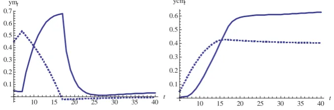
The dynamics under learning are shown in Figure 3 for the variables |w>

fw> qw> and lw (the mean paths over 20>000 replications are reported).9 The

solid black line illustrates the learning paths with the policy change. We also depict the learning paths without any policy change with the lighter shaded line. Of course, there are no dierences in the dynamics of the two economies for the rst year until the policy change is announced atw = 5= The severity of the recession during therst year means that |w has fallen by 5=61% as of w = 4= Once the policy change is announced at w = 5 the dynamics of the two economies starts to dier, though the eect on|w andfw for therst few periods is small.

The impact of the policy builds up steadily after the policy change comes into eect at w = 7. |w rises over time and is approximately 0=68 % points higher at w = 17. The dierences in dynamics start getting smaller from

w = 25 onwards but |w continues to be signicantly higher with the policy change for ve years and stays above the no-policy path throughout the 10 year period plotted in Figure 3. Employmentqwalso gets a substantial boost during the time of higherj and in fact is above the steady state from period

11 onwards. The boost in qw and the lower levels of fw during the time of higherj help explain the signicant expansionary eects of thescal policy under learning.10

We also plot the corresponding output multipliers for this policy exper-iment in Figure 4. The left hand panel shows the distributed lag multiplier and the right hand panel the (discounted) cumulative output multipliers. In thegure, the solid black line illustrates the multipliers under learning while the dashed line are the multipliers under the assumption of RE. The output

Cogan, Cwik, Taylor, and Wieland (2010).

9_{The policy we consider now is an announced anticipated change inj that takes place}

in the near future. For brevity we do not provide the details for RE and learning and refer the reader to Mitra, Evans, and Honkapohja (2011).

10_{As discussed in Section 4, investment is to some extent crowded out during therst}

multipliers are higher under RE compared to learning untilw = 9= However, the onset of the higherj from w = 7 gives a signicant boost to the output multiplier under learning which goes above RE levels soon after the policy change and stays higher than RE for the entire period plotted in Figure 4. Atw= 40 the cumulative output multiplier under learning is0=63while that under RE only 0=4=

Although the multipliers under learning are somewhat smaller than in Section 4, a scal stimulus is clearly eective in raising output and em-ployment during the recession. Yet again it is seen that the assumption of RE underestimates the eectiveness of scal policy when agents are learning adaptively over time. Fiscal policy can be quite eective in the standard RBC model not only when adopted during normal times but also when un-dertaken during recessionary times. This is particularly striking, given that our model does not include price or wage rigidities or liquidity constrained households.

6

Fiscal Consolidation

Since the 1990s there has been signicant interest in the so-called “non-Keynesian” eects ofscal policy spurred on by the seminal contribution of Giavazzi and Pagano (1990) who studied the two largestscal consolidations of the 1980s, Denmark in 1983-86 and Ireland in 1987-89. A striking feature of these contractionary scal policies was that the private sector boomed rather than fell into the deep recession that many economists and policy makers had predicted. A voluminous literature arose pointing to examples of scal consolidations (i.e. permanent reductions in government spending) displaying similar “non-Keynesian” eects.11

While the empirical literature is vast, there have been some attempts to explain these eects at a theoretical level, including discussion of whether spe-cial theories were needed to explain the eects of largescal consolidations. Most of the focus of this literature has been on an explanation of the eects of scal policy on private consumption.12 More recently, Alesina, Ardagna,

11_{For recent discussion and references, see Hemming, Kell, and Mahfouz (2002), Alesina,}

Perotti, Tavares, Obstfeld, and Eichengreen (1998), Briotti (2005), and Alesina and Ardagna (2010).

12_{These attempts include Blanchard (1990), Bertola and Drazen (1993), and Perotti}

Perotti, and Schiantarelli (2002) have argued that descriptive evidence sug-gests that increases in private investment (rather than private consumption) explain a greater share of the response of private-sector GDP growth in large

scal consolidations.13 _{Theynd very little evidence that private investment}

reacts dierently during these large scal adjustments than in the “normal” circumstances. As they remark on p. 586, “This result questions the need for “special theories” for large versus small changes in scal policy.”

Episodes of large scal consolidations are good examples of situations which economic agents are unlikely to have experienced earlier in their life-times. As argued in the Introduction, in such situations it is plausible to replace RE by the assumption that agents gradually learn about eects of these policy changes. We will see that the standard RBC model with adaptive learning is able to explain the key features in the behavior of consumption

and investment during these scal episodes.

Fiscal consolidations are typically modeled as a surprise permanent re-duction in government purchases, starting from steady state at w = 0. We consider the following scenario. At the beginning of period w = 1> a pol-icy announcement is made that the level of government purchases will fall permanently from ¯j = 0=22 to ¯j0 _{= 0=20 (i.e. an almost 10% drop in j).}

The policy announcement is assumed to be credible and known to the agents with certainty. We believe this is a realistic assumption; drastic cuts in pur-chases are typically implemented when things turn very bad and the public understands that permanent adjustments are required.

The long run eects on the steady state of a decrease in government con-sumption are well-known: higher concon-sumption and lower levels of investment, output, labor, and capital. See e.g. Baxter and King (1993).

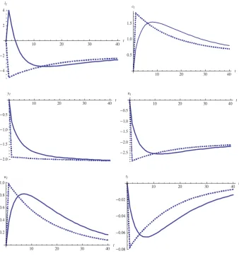
The dynamics under RE are also standard; see for instance Baxter and King (1993), pp. 321-2, Heijdra (2009), chapter 15, or Mitra, Evans, and Honkapohja (2011). The qualitative dynamics are conrmed by the behavior of variables under RE in Figure 5. For our purposes, the most relevant issue is the behavior of fw and lw. Under RE there is a big rise in fw on impact overshooting the new (higher) steady state followed by a gradual fall towards this steady state. lw> on the other hand, falls dramatically below the new (lower) steady state on impact followed by a gradual rise over time. While

13_{See also Alesina, Perotti, Tavares, Obstfeld, and Eichengreen (1998). Perotti (1999),}

the behavior offw is consistent with thescal episodes mentioned above, the behavior oflw is at odds with the empirical literature documented above.

Under learning fw rises on impact, followed by a gradual hump-shaped increase in its level eventually going above the RE level before monotonically falling towards the steady state. The most striking dierence from RE is, however, in the behavior of investment. Instead of the big drop in investment under RE, the opposite case of a large boom in investment and hence a rising path of capital occur under learning in the initial periods after the policy change. Strikingly, this qualitative behavior oflwunder learning is consistent with the empirical evidence cited above.

Why is the behavior of lw dierent under learning compared to RE? At w= 1, consumption rises because of the decrease in the present value of taxes

Vh

k>w. As in the case of a temporary change inj, discussed in Section 4, the impact eects are less under learning than under RE because the paths of futurezwanduw are not fully anticipated. Under learningzwh+v> uwh+vgradually respond to the data, leading initially to a gradual rise in zh

w+v (and fall in uh

w+v)before eventually falling towards the steady state.

As a consequence of the smaller sizes of the impacts on output and con-sumption at w = 1, the decrease in j necessarily leads to a higher level of

lw under learning than under RE, and in fact a sharp increase in investment follows. In the periods immediately following the policy change, expecta-tions of wages and interest rates begin to adjust. Two factors are at work. The higher capital stock in the periods soon after the policy change leads to higher forecasts of future wages and lower forecasts of future interest rates and thus higher Vzh

w and lower Vuwh. This leads to a further increase in fw, and decreases inqw and |w, which results in decreases inlw from its high level at w = 1. After several periods this process moves nw to an downward path, accompanied by a rise inqw, and a decrease in nw@qw, driving zw downwards and uw upwards to their steady state values. The other factor at work is that over time coe!cient estimates under RLS learning gradually adjust in response to the shock and the evolution of the data. Eventually the coe! -cients converge to the values that correspond to the REE values at the new steady state, so that in the long run there is convergence to the new REE.

signicantly above RE levels for a sustained period. These results forlw and fw are obtained in the conventional RBC model under learning, without the need to introduce real frictions or distortionary taxes that are employed in Alesina, Ardagna, Perotti, and Schiantarelli (2002).

Table 1 summarizes the impact of learning on the behavior of investment, consumption and output. For each variable the Table gives, over dierent horizons, the dierence between the cumulative impact under learning and under RE. This dierence is particularly striking for investment. For exam-ple, overve years the cumulative dierence between the level of investment under learning and under RE amounts to 6.6% of steady state output or 31.9% of steady state investment. Overve and ten year horizons the cumu-lative eect on consumption is also greater under learning than under RE. It follows that the cumulative dierence between the level of output under learning and under RE, which is equal to the sums of the dierences for in-vestment and consumption, is also large over all three horizons. Over ten years this dierence amounts to over 7.5% of steady state output.

It should be noted, however, that scal consolidation leads to a fall in output and employment under both RE and learning.14 _{This is an}

unavoid-able consequence of the lower steady state level that necessarily accompanies a permanent reduction inj in the basic RBC model that we are using. How-ever, qw falls less rapidly under learning and is around 0=7 of a percentage point higher than RE levels after year one. This feature explains the higher levels of output under learning compared to RE levels for the entire 10 year period depicted in Figure 5 and summarized in Table 1.

To summarize, the literature on scal consolidation emphasizes the pos-sibility of positive eects on both private consumption and, especially, pri-vate investment resulting from permanent decreases in government spending. Adaptive learning provides a natural mechanism, operating through expecta-tions, for a surge in investment immediately following ascal consolidation. The perceived lower taxes leads to higher consumption and lower employ-ment through the usual wealth eect. Under learning wages rise less, and interest rates fall less than they do under RE, so that consumption rises more gradually and the higher level of personal saving leads to higher levels of investment over this period.

14_{Empirical evidence on aggregate eects is reviwed, e.g., in Briotti (2005) and IMF}

7

Conclusion

In this paper we have studied the impact of changes in government purchases in a standard RBC model with adaptive learning. Methodologically, our approach has been to assume that households understand the direct eects of announced changes in government purchases on their after-tax income, but have imperfect knowledge of the implications of the policy for the future paths of wages and interest rates. Expectations of these latter variables follow the adaptive learning approach in which agents estimate and update their forecasts using statistical learning rules.

Using this approach we study the implications for three inter-related ques-tions that have been a major focus of recent research. Our main nding is that the multiplier eects of government purchases in RBC models un-der learning are much larger than unun-der the standard rational expectations assumption, and are within the range found in empirical studies. Under adaptive learning there is less crowding out of consumption and there is sub-stantial crowding in of investment. We alsond thatscal policy, taking the form of temporary increases in government purchases, is eective in increas-ing output and employment durincreas-ing severe recessions. Finally, we have seen that the behavior of both consumption and investment under scal consol-idations better matches the stylized empirical facts when adaptive learning is incorporated into the RBC model.

References

Aiyagari, R. S., L. J. Christiano, and M. Eichenbaum (1992): “The Output, Employment, and Interest Rate Eects of Government Consump-tion,” Journal of Monetary Economics, 30, 73—86.

Alesina, A., and S. Ardagna (2010): “Large Changes in Fiscal Policy: Taxes versus Spending,” Tax Policy and the Economy, 24, 35—68.

Alesina, A., S. Ardagna, R. Perotti, and F. Schiantarelli (2002): “Fiscal Policy, Prots, and Investment,” American Economic Review, 92, 571—589.

Alesina, A., R. Perotti, J. Tavares, M. Obstfeld, and B. Eichen-green(1998): “The Political Economy of Fiscal Adjustments,”Brookings Papers on Economic Activity, 1, 197—248.

Auerbach, A., W. G. Gale, and B. H. Harris (2010): “Activist Fiscal Policy,”Journal of Economic Perspectives, 24, 141—164.

Barro, R. J., and R. G. King (1984): “Macroeconomic Eects from Government Purchases and Taxes,”The Quarterly Journal of Economics, 99, 817—839.

Barro, R. J., and C. J. Redlick (2011): “Macroeconomic Eects from Government Purchases and Taxes,”The Quarterly Journal of Economics, 126, 51—102.

Baxter, M., and R. G. King (1993): “Fiscal Policy in General Equilib-rium,” The American Economic Review, 83, 315—334.

Bertola, G., and A. Drazen (1993): “Trigger Points and Budget Cuts: Explaining the Eects of Fiscal Austerity,” American Economic Review, 83, 11—26.

Blanchard, O. J. (1990): “Can Severe Fiscal Contractions be Expan-sionary? A Tale of Two Small European Countries: Comment,” NBER Macroeconomics Annual, 1, 75—111.

Briotti, M. G. (2005): “Economic Reactions to Public Finance Consoli-dation: A Survey of the Literature,” Occasional paper no.38.

Campbell, J. Y. (1994): “Inspecting the Mechanism: An Analytical Ap-proach to the Stochastic Growth Model,”Journal of Monetary Economics, 33, 463—506.

Carceles-Poveda, E., and C. Giannitsarou (2008): “Asset Pricing with Adaptive Learning,” Review of Economic Dynamics, 11, 629—651.

Christiano, L., M. Eichenbaum, and S. Rebelo (2011): “When is the Government Spending Multiplier Large?,” Journal of Political Economy, 119, 78—121.

Coenen, G., C. J. Erceg, C. Freedman, D. Furceri, M. Kumhof, R. Lalonde, D. Laxton, J. Linde, A. Mourougane, D. Muir, S. Mursula, C. D. Resende, J. Roberts, W. Roeger, S. Snudden, M. Trabandt, and J. I. Veld (2012): “Eects of Fiscal Stimulus in Structural Models,”American Economic Journal: Macroeconomics, 4, 22— 68.

Cogan, J. F., T. Cwik, J. B. Taylor, and V. Wieland (2010): “New Keynesian versus Old Keynesian Government Spending Multipliers,” Jour-nal of Economic Dynamics and Control, 34, 281—295.

Eusepi, S., and B. Preston (2010): “Central Bank Communication and Expectations Stabilization,”American Economic Journal: Macroeco-nomics, 2, 235—271.

(2011): “Expectations, Learning and Business Cycle Fluctuations,”

American Economic Review, 101, 2844—2872.

Evans, G. W., and S. Honkapohja(2001): Learning and Expectations in Macroeconomics. Princeton University Press, Princeton, New Jersey.

(2011): “Learning as a Rational Foundation for Macroeconomics and Finance,” mimeo.

Evans, G. W., S. Honkapohja, and R. Marimon (2001): “Conver-gence in Monetary In ation Models with Heterogeneous Learning Rules,”

Evans, G. W., S. Honkapohja, and K. Mitra (2009): “Anticipated Fiscal Policy and Learning,” Journal of Monetary Economics, 56, 930— 953.

(2011): “Does Ricardian Equivalence Hold When Expectations are not Rational?,” Working paper nr. 1008, Centre for Dynamic Macroeco-nomic Analysis, University of St Andrews.

Giannitsarou, C.(2006): “Supply-Side Reforms and Learning Dynamics,”

Journal of Monetary Economics, 53, 291—309.

Giavazzi, F., and M. Pagano (1990): “Can Severe Fiscal Contractions be Expansionary? A Tale of Two Small European Countries,” NBER Macroeconomics Annual, 1, 75—111.

Hall, R. E.(2009): “By How Much Does GDP Rise If the Government Buys More Output?,” Brookings Papers on Economic Activity, pp. 183—231.

Heijdra, B. J. (2009): Foundations of Modern Macroeconomics. Oxford University Press, Oxford.

Hemming, R., M. Kell, and S. Mahfouz (2002): “The Eectiveness of Fiscal Policy in Stimulating Economic Activity- A Review of the Litera-ture,” Working paper nr. 02/208, International Monetary Fund.

IMF(2010): World Economic Outlook, October 2010. IMF Publication Ser-vices, Washington, D.C.

King, R. G., C. I. Plosser, and S. T. Rebello (1988): “Production, Growth and Business Cycles,” Journal of Monetary Economics, 21, 195— 232.

King, R. G., and S. T. Rebello (1999): “Resuscitating Real Business Cycles,” in Taylor and Woodford (1999), pp. 927—1007.

Leeper, E. M., N. Traum,and T. B. Walker(2011): “Clearing Up the Fiscal Multiplier Morass,” mimeo.

Long, Jr., J. B., and C. I. Plosser (1983): “Real Business Cycles,”

Journal of Political Economy, 91, 39—69.

Marcet, A., and J. P. Nicolini (2003): “Recurrent Hyperin ations and Learning,” American Economic Review, 93, 1476—1498.

Milani, F. (2007): “Expectations, Learning and Macroeconomic Persis-tence,” Journal Of Monetary Economics, 54, 2065—2082.

Mitra, K., G. W. Evans, and S. Honkapohja (2011): “Policy Change and Learning in the RBC Model,” Working paper nr. 1111, Centre for Dynamic Macroeconomic Analysis, University of St Andrews.

Orphanides, A., and J. C. Williams (2007): “Robust Monetary Policy with Imperfect Knowledge,” Journal of Monetary Economics, 54, 1406— 1435.

Perotti, R.(1999): “Fiscal Policy in Good Times and Bad,”The Quarterly Journal of Economics, 114, 1399—1436.

Preston, B.(2006): “Adaptive Learning, Forecast-based Instrument Rules and Monetary Policy,”Journal of Monetary Economics, 53, 507—535.

Ramey, V. A. (2011a): “Can Government Purchases Stimulate the Econ-omy?,” Journal of Economic Literature, 49, 673—685.

(2011b): “Identifying Government Spending Shocks: It’s All In The Timing,”The Quarterly Journal of Economics, 126, 1—50.

Romer, C. D., and J. Bernstein(2009): “The Job Impact of the Amer-ican Recovery and Reinvestment Plan,” mimeo.

Sargent, T. J. (1999): The Conquest of American In ation. Princeton University Press, Princeton NJ.

(2008): “Evolution and Intelligent Design,” American Economic Review, 98, 5—37.

Taylor, J., and M. Woodford (eds.) (1999): Handbook of Macroeco-nomics, Volume 1. Elsevier, Amsterdam.

TABLE

Cumulative 3 years 5 years 10 years Eects in % RLSRE RLSRE RLSRE

(Plw)@|¯ 6=91 6=61 5=28

(Pfw)@|¯ 1=09 0=19 2=29

(P|w)@|¯ 5=82 6=80 7=57

(Plw)@¯~ 33=35 31=91 25=48

(Pfw)@f¯ 1=84 0=32 3=87

Table 1: Cumulative eects on key variables of a scal consolidation. Cumulative dierence between eects under learning (RLS) and under

10 20 30 40 50 60 t

0.4

0.2 0.2

kt

10 20 30 40 50 60 t

4

2 2 4 6

it

10 20 30 40 50 60 t

0.8

0.6

0.4

0.2

ct

10 20 30 40 50 60 t

0.2 0.4 0.6 0.8 1.0 1.2

nt

10 20 30 40 50 60 t

0.2 0.4 0.6

yt

10 20 30 40 50 60 t

0.4

0.3

0.2

0.1 0.1

wt

10 20 30 40 50 60

t

0.2 0.4 0.6 ym_t

10 20 30 40 50 60 t

0.2 0.4 0.6 0.8 ycmt

10 20 30 40 50 60 t

0.4 0.3 0.2 0.1

consmt

10 20 30 40 50 60 t

0.4 0.3 0.2 0.1

conscm_t

10 20 30 40 50 60 t

1.0 0.5 0.5 1.0

invmt

10 20 30 40 50 60 t

0.4 0.2 0.2 invcm_t

10 20 30 40 t

6

5

4

3

2

1

yt

10 20 30 40 t

5

4

3

2

1

ct

10 20 30 40 t

2.0

1.5

1.0

0.5 0.5 1.0

nt

10 20 30 40 t

25

20

15

10

5

it

Figure 3: Dynamic paths showing the impact on major variables of a scal stimulus announced in the midst of the Great Recession. Mean paths over 20,000 simulations. The solid black line illustrates the learning paths with the policy change and the lighter shaded line the learning paths without the policy change. All variables are measured in percentage deviations from steady state values.

10 15 20 25 30 35 40 t

0.1 0.2 0.3 0.4 0.5 0.6 0.7 ym_t

10 15 20 25 30 35 40 t

0.1 0.2 0.3 0.4 0.5 0.6 ycm_t

10 20 30 40 t

4

2 2 4

i_t

10 20 30 40 t

0.5 1.0 1.5

c_t

10 20 30 40 t

2.0

1.5

1.0

0.5

yt

10 20 30 40 t

2.5

2.0

1.5

1.0

0.5

n_t

10 20 30 40 t

0.2 0.4 0.6 0.8 1.0

w_t

10 20 30 40 t

0.08

0.06

0.04

0.02

rt

www.st-and.ac.uk/cdma

ABOUT THE CDMA

The Centre for Dynamic Macroeconomic Analysis was established by a direct grant from the University of St Andrews in 2003. The Centre facilitates a programme of research centred on macroeconomic theory and policy. The Centre is interested in the broad area of dynamic macroeconomics but has particular research expertise in areas such as the role of learning and expectations formation in macroeconomic theory and policy, the macroeconomics of financial globalization, open economy macroeconomics, exchange rates, economic growth and development, finance and growth, and governance and corruption. Its affiliated members are Faculty members at St Andrews and elsewhere with interests in the broad area of dynamic macroeconomics. Its international Advisory Board comprises a group of leading macroeconomists and, ex officio, the University's Principal.

Affiliated Members of the School

Dr Fabio Aricò.

Prof George Evans (Co-Director). Dr Gonzalo Forgue-Puccio. Dr Laurence Lasselle. Dr Seong-Hoon Kim. Dr Peter Macmillan. Prof Rod McCrorie.

Prof Kaushik Mitra (Director). Dr Geetha Selvaretnam. Dr Ozge Senay. Dr Gary Shea. Dr Gang Sun. Prof Alan Sutherland. Dr Alex Trew.

Senior Research Fellow

Prof Andrew Hughes Hallett, Professor of Economics, Vanderbilt University.

Research Affiliates

Prof Keith Blackburn, Manchester University. Prof David Cobham, Heriot-Watt University. Dr Luisa Corrado, Università degli Studi di Roma. Dr Tatiana Damjanovic, University of Exeter. Dr Vladislav Damjanovic, University of Exeter. Prof Huw Dixon, Cardiff University.

Dr Anthony Garratt, Birkbeck College London. Dr Sugata Ghosh, Brunel University.

Dr Aditya Goenka, Essex University. Dr Michal Horvath, University of Oxford. Prof Campbell Leith, Glasgow University. Prof Paul Levine, University of Surrey. Dr Richard Mash, New College, Oxford. Prof Patrick Minford, Cardiff Business School. Dr Elisa Newby, University of Cambridge. Prof Charles Nolan, University of Glasgow. Dr Gulcin Ozkan, York University.

Prof Joe Pearlman, London Metropolitan University. Prof Neil Rankin, Warwick University.

Prof Lucio Sarno, Warwick University.

Prof Eric Schaling, South African Reserve Bank and Tilburg University.

Prof Peter N. Smith, York University. Dr Frank Smets, European Central Bank. Prof Robert Sollis, Newcastle University. Dr Christoph Thoenissen, Victoria University of

Wellington and CAMA

Prof Peter Tinsley, Birkbeck College, London. Dr Mark Weder, University of Adelaide.

Research Associates

Miss Jinyu Chen. Mr Johannes Geissler. Miss Erven Lauw Mr Min-Ho Nam.

Advisory Board

Prof Sumru Altug, Koç University. Prof V V Chari, Minnesota University. Prof John Driffill, Birkbeck College London. Dr Sean Holly, Director of the Department of Applied

Economics, Cambridge University. Prof Seppo Honkapohja, Bank of Finland and

Cambridge University.

Dr Brian Lang, Principal of St Andrews University. Prof Anton Muscatelli, Heriot-Watt University. Prof Charles Nolan, St Andrews University.

Prof Peter Sinclair, Birmingham University and Bank of England.

Prof Stephen J Turnovsky, Washington University. Dr Martin Weale, CBE, Director of the National

www.st-and.ac.uk/cdma RECENT WORKING PAPERS FROM THE

CENTRE FOR DYNAMIC MACROECONOMIC ANALYSIS

Number Title Author(s)

CDMA10/13 Economic Crisis and Economic Theory Mark Weder (Adelaide, CDMA and

CEPR)

CDMA10/14 A DSGE Model from the Old

Keynesian Economics: An Empirical Investigation

Paolo Gelain (St Andrews) and Marco Guerrazzi (Pisa)

CDMA10/15 Delay and Haircuts in Sovereign Debt:

Recovery and Sustainability Sayantan Ghosal (Warwick), Marcus Miller (Warwick and CEPR) and Kannika Thampanishvong (St Andrews)

CDMA11/01 The Stagnation Regime of the New

Keynesian Model and Current US Policy George W. Evans (Oregon and St Andrews)

CDMA11/02 Notes on Agents' Behavioral Rules Under Adaptive Learning and Studies of Monetary Policy

Seppo Honkapohja (Bank of England), Kaushik Mitra (St Andrews) and George W. Evans (Oregon and St Andrews)

CDMA11/03 Transaction Costs and Institutions Charles Nolan (Glasgow) and Alex Trew (St Andrews)

CDMA11/04 Ordering Policy Rules with an

Unconditional Tatjana Damjanovic (St Andrews), Vladislav Damjanovic (St Andrews) and Charles Nolan (Glasgow)

CDMA11/05 Solving Models with Incomplete Markets and Aggregate Uncertainty Using the Krusell-Smith Algorithm: A Note on the Number and the Placement of Grid Points

Michal Horvath (Oxford and CDMA)

CDMA11/06 Variety Matters Oscar Pavlov (Adelaide) and Mark

Weder (Adelaide, CDMA and CEPR)

CDMA11/07 Foreign Aid-a Fillip for Development or

a Fuel for Corruption? Keith Blackburn (Manchester) and Gonzalo F. Forgues-Puccio (St Andrews)

CDMA11/08 Financial intermediation and the international business cycle: The case of small countries with big banks

www.st-and.ac.uk/cdma

CDMA11/09 East India Company and Bank of

England Shareholders during the South Sea Bubble: Partitions, Components and Connectivity in a Dynamic Trading Network

Andrew Mays and Gary S. Shea

CDMA11/10 A Social Network for Trade and Inventories of Stock during the South Sea Bubble

Gary S. Shea (St Andrews)

CDMA11/11 Policy Change and Learning in the RBC

Model Kaushik Mitra (St Andrews and CDMA), George W. Evans (Oregon and St Andrews) and

Seppo Honkapohja (Bank of Finland)

CDMA11/12 Individual rationality, model-consistent

expectations and learning Liam Graham (University College London)

CDMA11/13 Learning, information and heterogeneity Liam Graham (University College London)

CDMA11/14 (Re)financing the Slave Trade with the Royal African Company in the Boom Markets of 1720

Gary S. Shea (St Andrews)

CDMA11/15 The financial accelerator and monetary

policy rules GuThoenissen ̈neş Kamber and Christoph

CDMA11/16 Sequential Action and Beliefs under Partially Observable DSGE

Environments

Seong-Hoon Kim

CDMA12/01 A Producer Theory with Business Risks Seong-Hoon Kim and Seongman

Moon

..

For information or copies of working papers in this series, or to subscribe to email notification, contact:

Kaushik Mitra