ISSN 0962-4031
UNIVERSITY OF ST. ANDREWS
Optimal Climate Change Policies When
Governments Cannot Commit
(
Revised Version
)
Alistair Ulph
(University of Manchester)
David Ulph
No.1104
DISCUSSION PAPER SERIES
School of Economics & Finance
St. Salvator's College
St. Andrews, Fife KY16 9AL
Optimal Climate Change Policies When Governments
Cannot Commit
1Alistair Ulph
2and
David Ulph
3Abstract
We analyse the optimal design of climate change policies when a government wants to encourage the private sector to undertake significant immediate investment in developing cleaner technologies, but the relevant carbon taxes (or other environmental policies) that would incentivise such investment by firms will be set in the future. We assume that the current government cannot commit to long-term carbon taxes, and so both it and the private sector face the possibility that the government in power in the future may give different (relative) weight to environmental damage costs. We show that this lack of commitment has a significant asymmetric effect: it increases the incentive of the current government to have the investment undertaken, but reduces the incentive of the private sector to invest. Consequently the current government may need to use additional policy instruments – such as R&D subsidies – to stimulate the required investment.
JEL Nos: H23, Q54, Q55, Q58
Keywords: Climate Change; Emissions Taxes; Impact on R&D; Timing and Commitment
1 Earlier versions of this paper have been presented to the World Congress of Environmental and Resource
Economists, Montreal, 2010 and Towards Global Agreements on Environmental Protection and
Sustainability, Exeter 2011 as well as to workshops at ZEW Mannheim, SCI Manchester, Birmingham and St. Andrews. We are grateful to participants at these events, three referees, the editor, Partha Dasgupta and Nick Stern for comments. The usual disclaimer applies. (Revised Version of No.0909.)
2 Associate Vice-President and Executive Director of Sustainable Consumption Institute: Contact details:
Sustainable Consumption Institute, The University of Manchester, Manchester M13 9PL, UK. E-Mail:
3 Professor of Economics, University of St Andrews; Director, Scottish Institute for Research in Economics
(SIRE); Senior External Research Fellow, Centre for Business Taxation, University of Oxford.
1. Introduction
It is widely recognised4 that tackling inter-temporal environmental problems such as climate change will require a wide range of policy instruments, including both carbon pricing and policies to stimulate environmental R&D. The conventional economic argument why this is necessary is that there are multiple market failures – both environmental externalities and in the market for R&D. If there were no failures in the R&D market, and a single government chooses a time-path of policy instruments to maximize a welfare function over an infinite horizon, the resulting environmental policy instruments such as emissions/carbon taxes play a dual function: they induce the optimal level of emissions in every period, but they also give firms incentives to undertake investment (including investment in R&D) that will produce cleaner technologies. In this stylized framework, the major conclusion is that environmental policy instruments alone5 are sufficient to support the optimal R&D investment, output and emission paths6.
This simple argument breaks down if, as well as the environmental externality failure, there are other market failures, in particular in the market for R&D, and that the government lacks policy instruments to address these7. In this paper we assume that either such market failures do not exist8, or, equivalently, that governments have sufficient policy instruments to deal with these market failures. We focus instead on a different reason why the simple economic argument may not apply, which is that it pre-supposes that current governments can commit to future tax policies. But in a democratic system current governments may not be able to tie the hands of future governments on emission taxes9. There is now a significant literature on the possible ‘time inconsistency’ of environmental policies10. One reason why time inconsistency may arise is that there are some missing policy instruments, so that environmental policy is used to address more than one objective, for example equity issues as well as environmental issues, and
4 See for example the Stern (2007)
5 This is consistent with the conventional neoclassical notion of innovation being induced by changes in
relative prices (Jaffe, Newell and Stavins (2003)), in this case by changes in relative prices resulting from environmental policies.
6 One caveat is that his argument applies to marginal projects which bring about only incremental
improvements to the emissions technology and where it is consequently reasonable to assume that investors anticipate that emission taxes will be unaffected by their investment decisions. In this paper we will be concerned with R&D investments, which will bring about a radical improvement in the emissions technology and which consequently investors should anticipate will significantly lower emission taxes in the future. As we will discuss, this will generate too large an incentive to invest in R&D, and, even if there were a single government setting policy for all future time, it may need to set a tax on R&D to offset this effect.
7 Standard R&D market failures include capital market failures, appropriability problems, ‘rent-stealing’ –
see Jaffe et al (2003) for a survey. Other issues could include equity considerations (Abrego and Perroni (2002)) or imperfect competition (Helm, Hepburn and Mash (2003)) not addressed directly by other policies.
8 In the case of R&D we assume there is a single firm, so there are no spillover or strategic investment
issues, and this firm can fully capture all consumer benefits – so there are no undervaluation effects.
9
It is possible that joining an IEA may provide some commitment – but a country can leave an IEA. We discuss this further in the concluding section.
10 This literature draws on a much bigger literature on time-consistency in macro policy. See Brunner et al
this trade-off may be different ex post than ex ante. As already noted, in this paper we assume that governments have a full range of policy instruments to deal with other market failures, so this cannot provide a rationale for time inconsistency of environmental policy11. A second factor that could lead to time-inconsistency is when nations are involved strategically with other nations – for example through trade and environmental reasons. We deal with a single country so this source of time inconsistency cannot arise. It is sometimes argued that time inconsistency arises if a government commits to a future emission tax, firms invest in R&D to cut their emissions, and the government subsequently cuts the emission tax because costs of abatement have fallen. However, as we will show, this argument is incorrect; what a government should commit to is a tax policy, not a tax rate, and this policy will involve reducing the emission tax if the firm successfully innovates; indeed, in our model, the reduction in tax rate is part of the profit incentive for the firm to innovate12.
So, in our model, environmental policies will be time consistent, as long as future governments place the same weight on environmental considerations relative to other issues such as growth and employment as does the current government. But the lack of commitment matters if we take seriously the idea that future governments may have different objectives from the current government, in particular the weight they attach to environmental damages13. When firms contemplate their investment decisions they need to consider that future governments may place a greater or smaller (relative) weight on environmental damages, which will affect the taxes they impose. We show that this uncertainty about future governments’ preferences reduces firms’ incentives to invest14.
But how does uncertainty about future government’s environmental preferences affect the current government’s policies15? We show that lack of commitment increases the incentive for the government to have the investment undertaken – essentially because
11 Helm, Hepburn and Marsh (2003) note (footnote 1) that time inconsistency can be avoided by a full set
of policy instruments.
12 Ulph and Ulph (2001) show that if the government commits to a policy whereby the value of the policy
instrument depends on what investment decisions firms have made then welfare is always higher with commitment. In this paper if a government can commit (in the sense in which we use this term) it commits to a policy. See also Brunner et al (2011) for a good discussion of this point.
13 This ‘political volatility’ is the third factor identified by Brunner et al (2011) as a source of time
inconsistency. Golombek, Greaker and Hoel (2010), in a richer model of innovation than we use, confirm that if future governments have the same welfare function as the current government, then as long as the current government sets the optimal R&D policy (which need not be zero if there are R&D market failures) there is no time inconsistency in environmental policies. It could be argued that, in a democratic society, this is perhaps the most important source of potential time inconsistency.
14 The Stern Review notes that “Lack of certainty over the future pricing of the carbon externality will
reduce the incentive to innovate” Stern (2007) pp 393 and 399.
15 Boyer and Laffont (1999) analyse the trade-off that can arise if future governments have better
having a cleaner technology in place reduces the sensitivity of its objective function to the different policies that future governments might implement.
2. The Model
There is a single firm which produces a commodity the production/consumption of which generates pollution. Let x0 denote output; e0 emissions per unit of output, and
.
Ee x16 total emissions.
There are two periods. In period 1 the firm decides whether or not to make a fixed investment F > 0 in an environmental R&D project the sole benefit of which is to produce a cleaner technology. If the firm makes the investment, emissions per unit of output will be eL0, but if it does not, emissions per unit of output will remain at the
higher level eH eL, so that this investment makes a non-marginal change in emissions per unit of output. With a single firm there are no R&D spillovers and so there is no need for a policy instrument to correct that potential distortion. All the consumer benefits and environmental damage created by this firm accrue in period 217 and discounting is incorporated into the benefit and damage functions discussed below. In period 2 the firm chooses output, x, which yields consumer benefits B x( )0 (net of production costs),
( ) 0, ( ) 0
B x B x . To capture the idea that consumers are reluctant to cut back consumption we assume that demand is inelastic:
( )
( ) 1
( )
xB x x
B x
. (1)
To abstract from any competition issues arising from the potential exercise of monopoly power by this firm, we assume that the firm can perfectly price discriminate and thus capture consumer benefits B x( ). The damage cost function isD E( )0, where
(0) 0, ( ) 0, ( ) 0
D D E D E . The elasticity of the damage cost function is:
. ( )
( ) 0
( )
E D E E
D E
. (2)
Governments are in power for a single period and set policy only for the period in which they are in power and only in relation to decisions made by the firm in that period; in their objective functions they attach a weight ω to environmental damages relative to net consumer benefit. The government in period 1, which, without loss of generality, we assume has weight 1, cares about benefits and costs over both periods. However the only decision by the firm that the period 1 government can influence is whether or not it invests in R&D, and its only instrument is a lump-sum R&D subsidy S.18 The government in period 2, which may have weight 1, cares only about consumer
16 We ignore abatement to capture the idea that the main way of reducing emissions is new technology. 17 It may seem odd that in a model designed to capture a stock externality such as greenhouse gases we
assume emissions and damage occur only in one period. Our rationale is to focus on the idea that the key to reducing future environmental damage is innovation. We discuss this further in the concluding section.
18 This could be to profits or R&D. A profit subsidy conditioned on technology is equivalent to an R&D
benefits and damage costs in period 2 and can influence only the level of output, and hence emissions, chosen by the firm in period 2, which it does by a tax t per unit of emissions. The value of t chosen by the period 2 government depends on both its weight on environmental damages, ω, and on emissions per unit of output, and hence on the R&D decision made by the firm in period 1.
In this paper we say that the government in period 1 can commit if, in period 1, both it and the firm know for sure that the weight given to damages by the period 2 government is 1, so, in this sense, the ‘same’ government chooses both the period 1 R&D policy and the period 2 environmental policy. The government in period 1 cannot commit if both it and the firm recognize that the period 2 government may put a weight ω ≠ 1 on damage costs. We assume that they have a common probability density function f(ω) > 0, defined over an interval [0, ], > 1, for the value this weight might take, and that
E(ω) = 1, (the expected weight on environmental damages of the future government is no different from that of the current government). This captures the idea that the major consequence of lack of commitment is uncertainty about future government’s attitudes, rather than a systematic difference in attitude between current and future governments.
3. Analysis of the Model
We determine first the decisions of the government and firm in period 2 and then work backwards to determine the decisions of the government and firm in period 1.
3.1 Period 2: Output Decisions
Assume the second-period government has a weight, ω, on environmental damages, and that, as a result of its period 1 R&D decision, the firm’s technology has emissions e per unit of output. The period 2 government’s payoff is ( ) ( ). Let ˆ( , )x e be the output level that maximizes this payoff and Eˆ(e,)e.xˆ(e,) the associated level of total emissions. The first-order condition for the optimum output (marginal benefit equals marginal damage cost) is:
)) , ( ˆ . ( . ) , ( ˆ
(xe eD exe
B (3)
From (1), (2) and (3) the comparative static elasticities for output and emissions are:
ˆ ˆ ˆ
ˆ 1 ˆ 1
0 ˆ ˆ 1; ˆ 1 ˆ ˆ 0
ˆ ˆ
e x e E e x
x e E e x e
;
ˆ ˆ 1
0
ˆ ˆ ˆ ˆ
E x
x E
(4)
To induce the profit-motivated firm to choose the optimal output level the second-period
government sets an emissions tax equal to marginal damage. Let
x tex x B MAX e
t, ) [ ( ) ]
(
and ( , ) [ ( ) ]
x
x t e ARGMAX B x tex be, respectively, the maximum period 2 profits and the associated profit-maximising level of output of the firm when it faces an emissions tax and its emissions per unit of output are e. The first-order condition is
( , )
.B x t e t e. (5)
From (3) and (5), if the government sets an emission tax t eˆ( , ) D Eˆ( , ) e , then
̃[ ̂( ) ] ̂( ). (6) From (1) and (4) the comparative static elasticities of the emissions tax rate are:
ˆ ˆ
ˆ ˆ ˆ 1
. ˆ ˆ ˆ 0; ˆ
e t e E t e E e
ˆ ˆ ˆ ˆ ˆ ˆ 1 ˆ ˆ E E t t
>0 (7)
This shows that, given our assumption that demand is inelastic, if the firm introduces a cleaner technology, then the government sets a lower emission tax, while if the government attaches more weight to environmental damages, the tax rate will increase but less than proportionately.
3.2 Period 1: R&D Decisions.
In the first period the only decision to be made by the firm is whether or not to undertake the R&D investment. The only decision to be made by the government is how to use its R&D policy to align the firm’s decision with what it regards as socially optimal. It is assumed that, given the scale of the investment, both the firm and the government anticipate how the emissions tax (and hence output) will vary with both the emissions per unit of output and the weight the government in period 2 attaches to environmental damage costs. In this latter regard we need to distinguish the case of commitment from that of no commitment.
3.2.1 Commitment
To understand the implications for Period 1 policy of the government’s inability to commit, we establish the optimal policy in the benchmark case where both the firm and the government are certain that the government in period 2 gives a weight to environmental damage costs.
Let ˆc( )
ˆ( ,1)
. ( ,1)ˆ
( )
.x
W e B x e D e x e MAX B x D e x be the flow of net benefits
the period 1 government anticipates arising in period 2 if emissions per unit of output are
e and, in period 2, a government like it sets the emissions tax to maximize its payoff. The marginal gain from a reduction in e is:
ˆ
ˆ ˆ
ˆ( ,1) ( ,1) ˆ( ,1). ( ,1) 0
c
dW
x e D E e x e t e
de
Let ˆ2c( )e [ , ( ,1)]e t eˆ be the period 2 profits the firm will earn when its emissions per unit of output are e and it faces a government with weight = 1 imposing the emissions tax rate that it will regard as optimal. The firm’s incentive to reduce emissions per unit of output is :
2
ˆ ˆ ˆ
ˆ ˆ ˆ ˆ
. ( ,1) ( ,1) 1 ( ,1) ( ,1) 0; ˆ
c
d t e t
t e x e t e x e
de e t e t e
. (9)
So the firm sees two benefits from introducing a cleaner technology: (i) for a given emissions tax rate it lowers the tax on every unit of output; (ii) it anticipates that the government will lower the emissions tax. From (8) and (9) it is clear that the first of these effects alone is equivalent to the marginal social gain from a cleaner technology. This captures the idea that, if R&D investment was marginal, so that the firm treats the tax rate parametrically then emission taxes alone are sufficient to induce socially optimal R&D. However if the R&D investment is large, so the firm anticipates that future tax rates will depend on the emissions technology, the total marginal benefit to the firm from a cleaner technology exceeds that to the government, essentially because, by the convexity of the total damage cost function, the reduction in marginal damage costs (which determine the emission taxes) exceeds the reduction in average damage costs.
There are a number of equivalent policies for aligning public and private R&D returns. We suppose that in period 1 the government introduces a lump-sum profits subsidy conditioned on the emissions per unit of output: ̂( ) ̂( ) [ ̂( )]
[ ̂( )]. From (4) this is a strictly increasing function of e. If we let
1 2 ˆ
ˆc( ) ˆc( ) ( )
e e S e
be the total profits the firm anticipates in period 1 that it will make
if its emissions per unit of output are e, then it is clear that ˆ ( )1 ˆ2 ( )
c c
e W e
and private
profits are now aligned with the government objective function for any value of e. We can now define ˆ1c ˆ1c
eL ˆ1c
eH and Wˆc Wˆc
eL Wˆc
eH as the increase in profits and the government’s objective function that, in period 1, the firm and the government respectively anticipate from undertaking R&D. We have:Proposition 1. If commitment is possible, and governments implement an emissions tax policy ̂( ) in period 2 and a lump-sum subsidy policy19 ̂( ) in period 1, then for all
1 ˆ
ˆ
, c c
H L
e e W and so the private and social incentives to undertake R&D investment are identical.
Finally we note that the optimal R&D decision can also be implemented by any lump-sum policy ̂ ( ) ; in particular, let ̂ ( ), so the Period 1 government effectively imposes a lump-sum tax ̂ ̂ ( ) ̂ ( ) on R&D. This reflects the point noted above that the firm’s anticipated reduction in tax from lowering its emissions per unit of output exceeds the reduction in damages anticipated by the
19 These are policies since the governments are announcing how they will condition the particular value of
government, giving the firm too strong an incentive to invest, which, even with commitment, the government needs to correct by the lump-sum tax.
3.2.2 No Commitment
When the government in period 1 cannot commit, then, in period 1 both the firm and the government have to anticipate that the emission taxes set in period 2 will be chosen by a government that gives a weight ω ≠ 1 to environmental damage costs.
So let Wn
e, B x e
ˆ( , )
D ex eˆ( , )
be the payoff that the government in period 1 anticipates getting in period 2 when the firm has a technology with emissions per unit of output e and the period 2 policies will be implemented by a government with weight on environmental damages. Obviously:( ) ( ,1) 0
c n
W e W e e . (10)
From (3) and (4) it follows that
ˆ( , ) ˆ( , ) . ( , )
1
ˆ ˆ
n E e D E e
W e
, so
( , )
0 as 1 n
W e
. (11)
Thus, for any technology, the period 1 government’s payoff is maximized when it anticipates that future governments will act like it.
The period 1 government’s gain from lower emissions per unit of output is:
( , ) ˆ( , ) ˆ( , ) 1
1 ˆ ˆ
1 ˆn
W e
x e D E e e
. (12)
This reduces to (8) when . We are interested in how this varies with the weight put on damage costs by the second period government. From (4) the first term on the right hand side of (12) is a strictly decreasing function of ω, while, in the special case where the elasticities ̂ ̂ are constant, the right hand side is a strictly increasing function of ω. This suggests that the period 1 government’s desire to have R&D undertaken will be higher when the second period government is very different from itself, because the lower are emissions per unit of output the less will its objective function be affected by a future government’s setting what the period 1 government regards as the “wrong” taxes.
Similarly let ˆ2( , ) [ , ( , )]ˆ
n
e e t e
be the period 2 profits the firm will earn when its emissions per unit of output are e and the emission tax policy is chosen by a government that places a weight on environmental damage costs. From (3) and (7) it follows that:
so the firm’s profits are reduced by having a period 2 government which attaches a higher weight, and hence emission tax, on environmental damages. Analogous to (9), and using (7), the firm’s marginal gain in period 2 profits from lower emissions per unit of output is:
] ˆ( , )ˆ( , )[1 ˆ ˆˆ 1ˆ] 0
ˆ ˆ 1 )[ , ( ) , ( ˆ ˆ 2
t e x e
e t t e e x e t e n (14)
How does this marginal gain vary with ω? In the case where the elasticities ̂ ̂ are constant, then there are two effects: from (7) an increase in ω increases the tax rate, but, from (4) it reduces output. Given our assumption that ̂ , then, from (7) and (4), the first effect dominates the second so the marginal private incentive to invest in R&D is greater the larger is the weight put on damage by the second period government.
To understand whether the lack of commitment would cause the government in period 1 to implement a different policy from that it would follow under commitment, we first need to consider what the private incentive of the firm to invest in R&D would be if the period 1 government implemented the same R&D lump-sum subsidy policy as under commitment. In this case the total profits the firm would anticipate making over periods 1 and 2 would be ˆ1n( , )e ˆn2( , )e S eˆ( )
Recognising the discrete nature of investment, the gains to the period 1 government and the firm from R&D are Wn( ) W en( , )L W en( H, ) and
1 1 1
ˆn( ) ˆn( , ) ˆn( , )
L H
e e
respectively. Note that ˆ1n( ) ˆ2n( ) Tˆ where
2 2 2
ˆn( ) ˆn( , ) ˆn( , )
L H
e e
and, as before, TˆSˆ(eH)Sˆ(eL).
We need to understand the relationship between Wn( ) and ˆ ( )1
n
for all values of
. We know that ˆ1n(1) ˆc Wˆc Wn(1). It is straightforward to see that
2
ˆ (0) 0n
, because, when the government attaches no weight to environmental damages, Period 2 emission taxes are zero irrespective of the firm’s technology, so output and hence profits (i.e. consumer benefits) will be the same whether or not the firm has innovated. Consequently ˆ (0)1n Tˆ 0. However for the government W1(0)0, because the payoff gain to the government is the difference between the damage costs incurred when the firm produces that common level of output with and without the new technology. In addition, we can show20 that, under plausible assumptions,
(0) (1) 0
n n
W W
.
20 Define x~x(0)Then: 1(0) 1(1) {[ ( ) ( )] [ ( ˆ(1, )) ( ˆ(1, ))}
H L H
H L
Hx De x De x e De x e
e D W
W
)]}. , 1 ( ˆ [ )] , 1 ( ˆ [ { )]} , 1 ( ˆ [ )] , 1 ( ˆ [
{B x eL B x eH DeLx eL DeLx eH
It is difficult to make further progress on the analysis of uncertainty with general forms for the benefit and damage cost functions so we now make the stronger assumption that the elasticities
x , ( ) E are constant, denoted and respectively. It can be shown21 that, ignoring a common constant term,( ) [ ] /
n
W
(12a)
2
ˆ ( )n
(12b)
where
1, 1 0 < γ, η < 1.
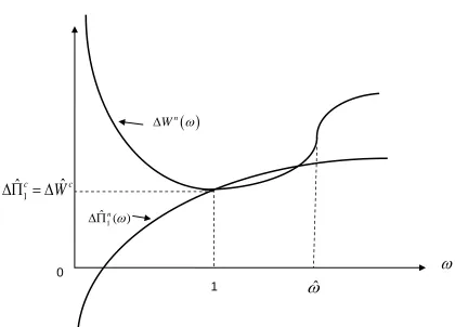
The key features of these functions are summarized in the following Lemma:
Lemma (i) n()
W
takes a minimum at 1 and is convex over an interval [0, ~ ] where ~ >2;
for n( )
W
is increasing and concave; (1) ( ) 1
(1 )
n
W
;
(ii) ˆ ( )2
n
is zero when 0, strictly increasing and concave; ˆ (1) 12 (1)
n n
W
; (iii) ˆ ( )1n is strictly increasing and concave; ˆ1n(0) Tˆ; ˆ1n(1) Wn(1)22.
These features are illustrated in Figure 1. The intuition for (i) is that the lower are emissions per unit of output the less sensitive is the welfare of the period-1 government to the type of government that is in power in period 2, so the greater is its incentive to have the cleaner technology in place the more different is a future government from itself; and for (ii), although emission taxes increase with the weight on damage costs, they do so at a decreasing marginal rate because the firm responds by cutting emissions (and hence output).
From the above Lemma and our assumption that E( ) 1 so that, on average, future governments give the same weight to damage costs as the current government we can establish the following:
Proposition 2
Uncertainty regarding the weight placed on damage by future governments: (i) increases the government’s gain from R&D: E[Wn( )] Wn(1) Wˆc; (ii) reduces the firm’s incentive to undertake R&D: [ ˆ1( )] ˆ1(1) ˆ1
n n c
E ;
desired emissions tax. The second term is negative because output will be higher if firms undertook the investment. The final term is positive reflecting the fact that, conditional on the firm using the cleaner technology, this carries the downside of higher emissions. We assume that x is sufficiently large that the first term dominates.
21
The results are in a technical appendix available from the authors.
22 From (12) and parts (i) and (ii) it follows that ̂ ( )
(iii)from which it follows that E[Wn( )] E[ ˆ1n( )] and so, to align private and public R&D incentives the government in period 1 needs to introduce an R&D ‘no commitment subsidy’.
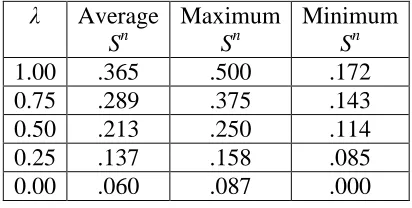
We define Sn E{[Wn()]E[1n()]}/ˆ1c as the required ‘no commitment subsidy’ expressed as a proportion of the profits the firm would earn with commitment. While Proposition 2 establishes our argument that the inability of governments to commit warrants a subsidy to R&D to align public and private incentives to invest, how large would Sn need to be? We have used the functional forms in (12), and assume that ω is distributed over the range [0,2] with density function f():
1 0
) 1 ( 5 . 0 )
(
f (13a)
2 1
) 1 ( 5 . 1 2 )
(
f (13b)
where 01. If 1, f()is the uniform density function; if 0, f()is the triangular density function; for intermediate values of , f()is a linear combination of a uniform and triangular density function23. In the appendix we derive the resulting value for Sn for any value of λ, β and δ. We have taken values of λ between 0 and 1, and for each value of λ we have run a million Monte Carlo simulations in which values of β and δ are drawn from uniform distributions lying in the intervals [1, 3] and [0.1, 3] respectively. Table 1 shows as λ falls from 1 to 0 the average, maximum and minimum values of Snall fall, but the subsidies are significant, with the average subsidy lying between 6% and 36%, the maximum between 9% and 50%, and the minimum between 0% and 17%.
In summary, we have shown that if governments cannot commit to future environmental policies then uncertainty about future governments’ weights on environmental damages could justify significant R&D subsidies to ensure that large-scale environmental investments are undertaken.
4. Conclusions
We have shown that the inability of governments to commit to policies calls into question the traditional prescription that environmental policies alone are sufficient to induce both optimal emissions and optimal investment in R&D. This is because the inability of the current government to commit to future emission taxes increases the wish of the current government that the private sector undertakes the investment but reduces the private sector’s incentive to invest. Numerical simulations show that the required subsidies are not trivial.
In demonstrating this result we have employed a very simple model. One issue is whether there may be other mechanisms by which a current government could make commitments, avoiding the need for an R&D subsidy. A number of such possibilities have been proposed in the literature: delegation of environmental policy to an independent agency (analogous to independence of central banks in monetary policy)24;
using tradable permits linked to a financial instrument with a put option which guarantees a floor to the future price for permits25. However, neither is straightforward26, particularly in the context of a long-term problem such as climate change. For example, as we have shown, any future emission tax or permit price should be made contingent on what innovation has been carried out, so defining an appropriate floor price could be difficult; while delegation has been successful for short-term monetary policy, it would be more problematic for long-term environmental problems. Ultimately future governments could disband any such devices. A subsidy to environmental R&D by current governments is arguably a more secure way of offsetting industry’s concerns about investing in such projects.
The second issue is how robust our results would be in a richer model. One obvious extension would be to model a proper stock-externality problem with emissions also in Period 1; it is an interesting conjecture whether this could lead the Period 1 government to set too low an emission tax in Period 1 to force the Period 2 government to take more action. A further extension would be to study a multi-country problem and consider whether joining an IEA gives a form of commitment to future emissions policy. Finally we have ignored intrinsic uncertainty about the climate change process with the related issue of how the possibility of getting better information in the future about climate change damages affects current period policy in a world where governments cannot commit.
25 See Ismer and Neuhoff (2009) for a thorough discussion.
References
Abrego, L. and C. Perroni (2002): “Investment Subsidies and Time-Consistent
Environmental Policy”, Oxford Economic Papers, 54(4), 617-635. Boyer, M. and J-J Laffont (1999): “Towards a Theory of the Emergence of
Environmental Incentive Regulation”, Rand Journal of Economics, 30, 137-157. Brunner, S., C. Flachsland and R. Marcschinski (2011): “Credible Commitment in
Carbon Policy”, Climate Policy (forthcoming)
Golombek, R., M. Greaker and M. Hoel (2010): “Climate Policy without Commitment”
CESifo Working Paper No 2909.
Helm, D., C. Hepburn and R. Mash (2003): “Credible Carbon Policy”, Oxford Review of Economic Policy, 19(3), 438-450.
Ismer, R. and K. Neuhoff (2009): “Commitments Through Financial Options: an
Alternative for Delivering Climate Change Obligations”, Climate Policy, 9, 9-21. Jaffe, A., R. Newell and R. Stavins (2003): “Technological Change and the
Environment”, in K. Maler and J. Vincent (eds.) Handbook of Environmental Economics, North-Holland, Amsterdam, 461-516.
Petrakis, E. and A. Xepapadeas (2000): "Location Decisions, Environmental Policy and Government Commitment", in N. Georgantzis and I. Barreda (eds.), Spatial Economics and Ecosystems: The Interaction Between Economics and the Natural Environment, Series: Advances in Ecological Sciences WIT (Wessex Institute of Technology) Press. pp. 115-127.
Stern, N. (2007): Stern Review of the Economics of Climate Change, HM Treasury Ulph, A. and D. Ulph (1997), “Global Warming, Irreversibility and Learning”, Economic
Journal, 107, 636-650.
Ulph, A. and D. Ulph (2001) “Strategic Trade and Industrial Policy in Dynamic
Figure 1 Graphs of
Wn( ) and ˆ ( )1n
1
ˆ
ˆ
c cW
0
1
1
ˆ ( )n
nW
Table 1 Values of Non-Commitment Subsidy, Sn
λ Average
Sn
Maximum
Sn
Minimum
Sn
1.00 .365 .500 .172
0.75 .289 .375 .143
0.50 .213 .250 .114
0.25 .137 .158 .085